Intervention liquidity effects #
This notebook serves as an illustration of the points discussed in the updated post based on the original post “Intervention liquidity” available on the Macrosynergy website.
This notebook provides the essential code required to replicate the analysis discussed in the post.
The notebook covers the three main parts:
-
Get Packages and JPMaQS Data: This section is responsible for installing and importing the necessary Python packages used throughout the analysis.
-
Transformations and Checks: In this part, the notebook performs calculations and transformations on the data to derive the relevant signals and targets used for the analysis, including the normalization of feature variables using z-score or building simple linear composite indicators.
-
Value Checks: This is the most critical section, where the notebook calculates and implements the trading strategies based on the hypotheses tested in the post. This section involves backtesting a few simple but powerful trading strategies targeting selected financial returns.
Note that while the notebook focuses on a selection of indicators and strategies underlying the post’s main findings, users are encouraged to explore numerous other indicators and approaches. The code can be adapted to test different hypotheses and strategy variations based on your research and ideas. Best of luck with your research!
Get packages and JPMaQS data #
This notebook primarily relies on the standard packages available in the Python data science stack. However, there is an additional package,
macrosynergy
, that is required for two purposes:
-
Downloading JPMaQS data: The
macrosynergypackage facilitates the retrieval of JPMaQS data, which is required in the notebook. -
For the analysis of quantamental data and value propositions: The
macrosynergypackage provides functionality for performing quick analyses of quantamental data and exploring value propositions.
For detailed information and a comprehensive understanding of the
macrosynergy
package and its functionalities, please refer to the
“Introduction to Macrosynergy package”
notebook on the Macrosynergy Quantamental Academy or visit the following link on
Kaggle
.
#! pip install git+https://github.com/macrosynergy/macrosynergy@develop
import pandas as pd
import os

import macrosynergy.management as msm
import macrosynergy.panel as msp
import macrosynergy.signal as mss
import macrosynergy.pnl as msn
import macrosynergy.visuals as msv

from macrosynergy.download import JPMaQSDownload
from macrosynergy.management.types import QuantamentalDataFrame

import warnings
warnings.simplefilter("ignore")
The JPMaQS indicators we consider are downloaded using the J.P. Morgan Dataquery API interface within the
macrosynergy
package. This is done by specifying ticker strings, formed by appending an indicator category code
DB(JPMAQS,<cross_section>_<category>,<info>)
, where
value
giving the latest available values for the indicator
eop_lag
referring to days elapsed since the end of the observation period
mop_lag
referring to the number of days elapsed since the mean observation period
grade
denoting a grade of the observation, giving a metric of real-time information quality.
After instantiating the
JPMaQSDownload
class within the
macrosynergy.download
module, one can use the
download(tickers,start_date,metrics)
method to easily download the necessary data, where
tickers
is an array of ticker strings,
start_date
is the first collection date to be considered and
metrics
is an array comprising the times series information to be downloaded. For more information see
here
# Developed and emerging markets

cids_dm = ["AUD", "CAD", "CHF", "EUR", "GBP", "JPY", "NOK", "NZD", "SEK", "USD"]
cids_em = [
    "BRL",
    "CLP",
    "CNY",
    "COP",
    "CZK",
    "HUF",
    "IDR",
    "ILS",
    "INR",
    "KRW",
    "MXN",
    "MYR",
    "PEN",
    "PHP",
    "PLN",
    "RON",
    "RUB",
    "SGD",
    "THB",
    "TRY",
    "TWD",
    "ZAR",
]
cids = cids_dm + cids_em

# Exclusions for illiquidity or restricted trading
cids_wild = ["CNY", "RUB"]
cids_il = sorted(set(cids) - set(cids_wild))

# FX-specific list
cids_fx = sorted(set(cids_il) - set(["EUR", "USD", "SGD"]))

# Equity-specific lists
cids_dmeq = ["AUD", "CAD", "CHF", "EUR", "GBP", "JPY", "SEK", "USD"]
cids_emeq = ["BRL", "INR", "KRW", "MXN", "MYR", "PLN", "SGD", "THB", "TRY", "TWD", "ZAR"]
cids_eq = cids_dmeq + cids_emeq
cids_eq.sort()

# Duration-specific lists
cids_dmdu = [
    "AUD",
    "CAD",
    "CHF",
    "EUR",
    "GBP",
    "JPY",
    "NOK",
    "NZD",
    "SEK",
    "USD",
]
cids_emdu = [
    "BRL",
    "CLP",
    "COP",
    "CZK",
    "HUF",
    "IDR",
    "ILS",
    "INR",
    "KRW",
    "MXN",
    "MYR",
    "PLN",
    "SGD",
    "THB",
    "TRY",
    "TWD",
    "ZAR",
]
cids_du = cids_dmdu + cids_emdu

cids_eqdu = [cid for cid in cids_eq if cid in cids_du]
cids_dmeqdu = [cid for cid in cids_dmeq if cid in cids_du]

# Categories

main = [
    # Intervention-driven liquidity expansion as % of GDP
    "INTLIQGDP_NSA_D1M1ML1",
    "INTLIQGDP_NSA_D1M1ML3",
    "INTLIQGDP_NSA_D1M1ML6",
    # Monetary base expansion as % of GDP
    "MBASEGDP_SA_D1M1ML1",
    "MBASEGDP_SA_D1M1ML3",
    "MBASEGDP_SA_D1M1ML6",
]  # liquidity indicators

#
econ = [
    "USDGDPWGT_SA_3YMA",
    "INFE1Y_JA",

]

rets = [
    "DU05YXR_VT10",  # Duration return, for 10% vol target: 5-year maturity
    "DU05YXR_NSA", # Duration return, 5-year maturity
    "EQXR_NSA",  # Equity index future returns in % of notional
    "EQXR_VT10",  # Equity index future return for 10% vol target
    "FXXR_VT10",  # FX forward return for 10% vol target: dominant cross
    "FXXRHvGDRB_NSA",  # Return on FX forward, hedged against market direction risk
    "FXTARGETED_NSA",  # Exchange rate target dummy
    "FXUNTRADABLE_NSA",  # Exchange rate untradable dummy
]  # returns

xcats = main + rets + econ

# Resultant tickers

tickers = [cid + "_" + xcat for cid in cids for xcat in xcats]
print(f"Maximum number of tickers is {len(tickers)}")
Maximum number of tickers is 512
#  Download series from J.P. Morgan DataQuery by tickers

start_date = "1990-01-01"

# Retrieve credentials
client_id: str = os.getenv("DQ_CLIENT_ID")
client_secret: str = os.getenv("DQ_CLIENT_SECRET")

with JPMaQSDownload(client_id=client_id, client_secret=client_secret) as dq:
    df = dq.download(
        tickers=tickers,
        start_date=start_date,
        suppress_warning=True,
        metrics=["value"],
        show_progress=True,
    )

dfx = df.copy() # copy to preserve original df in offline mode
Downloading data from JPMaQS.
Timestamp UTC:  2025-08-27 12:48:43
Connection successful!
Requesting data: 100%|██████████| 26/26 [00:05<00:00,  4.93it/s]
Downloading data: 100%|██████████| 26/26 [00:27<00:00,  1.06s/it]
Some expressions are missing from the downloaded data. Check logger output for complete list.
34 out of 512 expressions are missing. To download the catalogue of all available expressions and filter the unavailable expressions, set `get_catalogue=True` in the call to `JPMaQSDownload.download()`.
JPMaQS indicators are conveniently grouped into seven main categories: Economic Trends, Macroeconomic balance sheets, Financial conditions, Shocks and risk measures, Stylized trading factors, Economic surprises, and Generic returns. The description of each JPMaQS category is available under Macro quantamental academy . For tickers used in this notebook see Intervention liquidity , Duration returns , Equity index future returns , FX forward returns , and FX tradeability and flexibility .
This notebook defines several currency lists for convenience in analysis:
-
cids_dm: developed market currencies -
cids_em: emerging market currencies -
cids_il: investable universe: all unique currencies from cids_dm and cids_em, excluding CNY and RUB -
cids_fx: FX trading universe from cids_il excluding the base currencies USD, EUR and SGD -
cids_eq: subset of cids_dm and cids_em with available equity return data, built as cids_dmeq ∪ cids_emeq (developed equity markets and emerging equity markets) -
cids_du: currencies with duration return coverage, built as cids_dmdu ∪ cids_emdu (developed and emerging markets) -
cids_eqdu: intersection used for strategies needing both equity and duration (cids_eq ∩ cids_du) -
cids_dmeqdudeveloped-only intersection (cids_dmeq ∩ cids_dmdu)
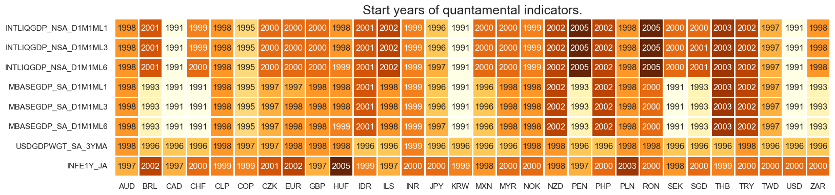
Availability #
xcatx = main + econ
msm.check_availability(dfx, xcats=xcatx, cids=cids_il, missing_recent=False),
(None,)
Blacklist dictionary #
Identifying periods of exchange rate targets, illiquidity, or convertibility distortions is a crucial first step in developing FX trading strategies. These distortions can heavily influence currency behaviour, and ignoring them risks flawed analysis. A standard blacklist (
fx_black
) can be used with various macrosynergy functions to exclude such periods from analysis.
dfb = dfx[dfx["xcat"].isin(["FXTARGETED_NSA", "FXUNTRADABLE_NSA"])].loc[
    :, ["cid", "xcat", "real_date", "value"]
]
dfba = (
    dfb.groupby(["cid", "real_date"])
    .aggregate(value=pd.NamedAgg(column="value", aggfunc="max"))
    .reset_index()
)
dfba["xcat"] = "FXBLACK"
fx_black = msp.make_blacklist(dfba, "FXBLACK")
fx_black
{'BRL': (Timestamp('2012-12-03 00:00:00'), Timestamp('2013-09-30 00:00:00')),
 'CHF': (Timestamp('2011-10-03 00:00:00'), Timestamp('2015-01-30 00:00:00')),
 'CNY': (Timestamp('1999-01-01 00:00:00'), Timestamp('2025-08-26 00:00:00')),
 'CZK': (Timestamp('2014-01-01 00:00:00'), Timestamp('2017-07-31 00:00:00')),
 'ILS': (Timestamp('1999-01-01 00:00:00'), Timestamp('2005-12-30 00:00:00')),
 'INR': (Timestamp('1999-01-01 00:00:00'), Timestamp('2004-12-31 00:00:00')),
 'MYR_1': (Timestamp('1999-01-01 00:00:00'), Timestamp('2007-11-30 00:00:00')),
 'MYR_2': (Timestamp('2018-07-02 00:00:00'), Timestamp('2025-08-26 00:00:00')),
 'PEN': (Timestamp('2021-07-01 00:00:00'), Timestamp('2021-07-30 00:00:00')),
 'RON': (Timestamp('1999-01-01 00:00:00'), Timestamp('2005-11-30 00:00:00')),
 'RUB_1': (Timestamp('1999-01-01 00:00:00'), Timestamp('2005-11-30 00:00:00')),
 'RUB_2': (Timestamp('2022-02-01 00:00:00'), Timestamp('2025-08-26 00:00:00')),
 'SGD': (Timestamp('1999-01-01 00:00:00'), Timestamp('2025-08-26 00:00:00')),
 'THB': (Timestamp('2007-01-01 00:00:00'), Timestamp('2008-11-28 00:00:00')),
 'TRY_1': (Timestamp('1999-01-01 00:00:00'), Timestamp('2003-09-30 00:00:00')),
 'TRY_2': (Timestamp('2020-01-01 00:00:00'), Timestamp('2024-07-31 00:00:00'))}
Transformations and checks #
Features #
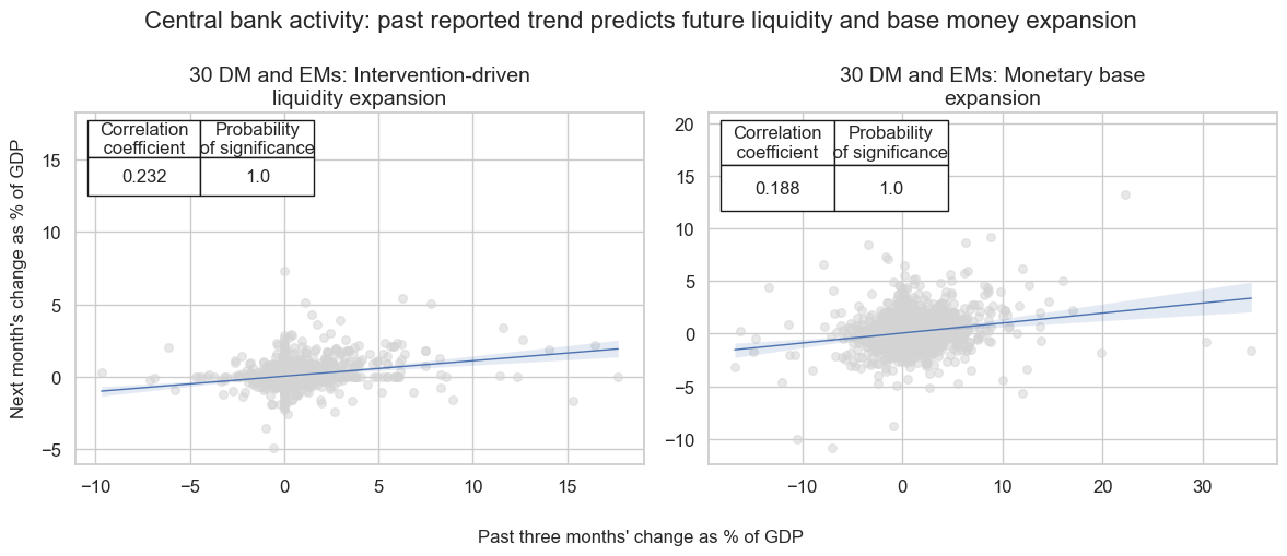
Visualize predictability of intervention liquidity #
# Show predictive power of past for future intervention trends

prefixes = ["INTLIQGDP_NSA", "MBASEGDP_SA"]
cr = {}

for prefix in prefixes:
    cidx = cids_il

    cr[f"cr_{prefix.lower()}_trend"] = msp.CategoryRelations(
        dfx,
        xcats=[f"{prefix}_D1M1ML3", f"{prefix}_D1M1ML1"],
        cids=cidx,
        freq="M",
        lag=1,
        xcat_aggs=["last", "last"],
        start="2000-01-01",
        xcat_trims=[None, 50],  # removes one vast outlier
    )

msv.multiple_reg_scatter(
    cat_rels=[cr["cr_intliqgdp_nsa_trend"], cr["cr_mbasegdp_sa_trend"]],
    ncol=2,
    nrow=1,
    figsize=(12, 5),
    coef_box="upper left",
    share_axes=False,
    title="Central bank activity: past reported trend predicts future liquidity and base money expansion",
    title_fontsize=16,
    subplot_titles=[
        f"{len(cids_il)} DM and EMs: Intervention-driven liquidity expansion",
        f"{len(cids_il)} DM and EMs: Monetary base expansion",
    ],
    xlab="Past three months' change as % of GDP",
    ylab="Next month's change as % of GDP",
)
Annualized country expansion rates #
# Annualized liquidity expansion across countries (long runtime)

cidx = cids_il
cbals = ["INTLIQGDP_NSA", "MBASEGDP_SA"]
calcs = []

for cbal in cbals:
    calcs.append(f"{cbal}_D1M1ML6AR = {cbal}_D1M1ML6 * 2")
    calcs.append(f"{cbal}_D1M1ML3AR = {cbal}_D1M1ML3 * 4")
    calcs.append(f"{cbal}_D1M1ML1AR = {cbal}_D1M1ML1 * 12")

dfa = msp.panel_calculator(df=dfx, calcs=calcs, cids=cidx)
dfx = msm.update_df(dfx, dfa)

# Cross-horizon composites

changes = ["D1M1ML1AR", "D1M1ML3AR", "D1M1ML6AR"]
composites = {
    "INTLIQGDP_NSA_DAR": ["INTLIQGDP_NSA_" + chg for chg in changes],
    "MBASEGDP_SA_DAR": ["MBASEGDP_SA_" + chg for chg in changes],
}

for new_xcat, dars in composites.items():
    dfa = msp.linear_composite(
        df=dfx,
        xcats=dars,
        cids=cids_il,
        complete_xcats=False,
        new_xcat=new_xcat,
    )
    dfx = msm.update_df(dfx, dfa)

# collect annualized liquidity expansion rates and their composites in one list

cbal_dars = [
    f"{cbal}_{dar}"
    for cbal in cbals
    for dar in ["D1M1ML6AR", "D1M1ML3AR", "D1M1ML1AR", "DAR"]
]

# calculate excess liquidity expansion rates and collect in one list

for cbal_dar in cbal_dars:
    calcs += [f"X{cbal_dar} = ( {cbal_dar} - INFE1Y_JA )"]

dfa = msp.panel_calculator(dfx, calcs=calcs, cids=cidx)
dfx = msm.update_df(dfx, dfa)

xcbal_dars = [f"X{cbal_dar}" for cbal_dar in cbal_dars]
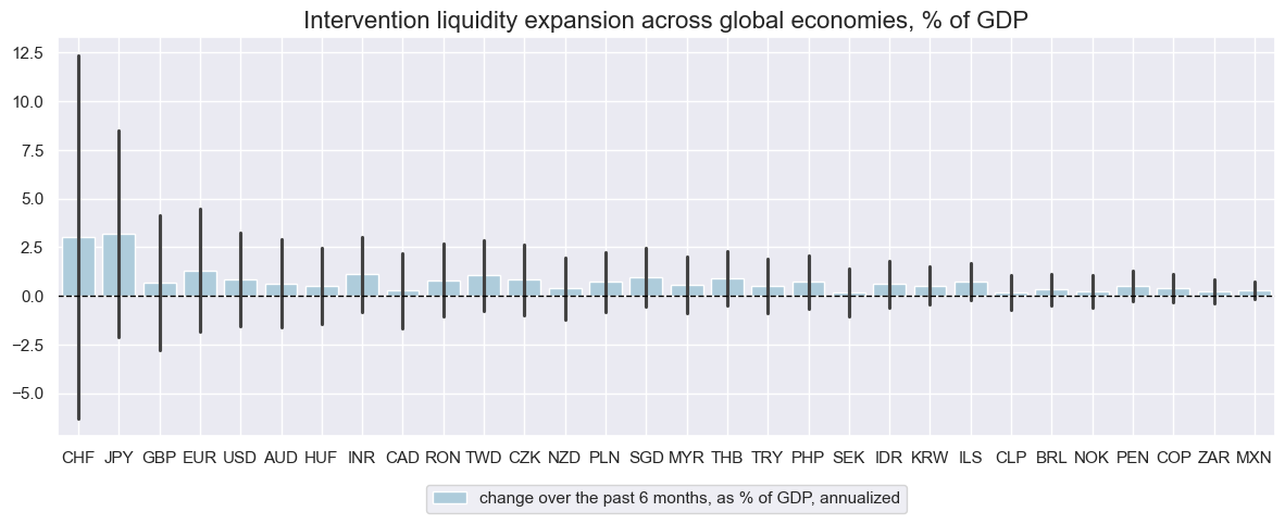
# Visualized growth rates by country
xcx = "INTLIQGDP_NSA"
xcatx = [xcx + "_" + dar for dar in ["D1M1ML6AR", "D1M1ML3AR", "D1M1ML1AR"]]
cidx = cids_il
dict_labs = {
xcx + "_D1M1ML6AR": "change over the past 6 months, as % of GDP, annualized",
xcx + "_D1M1ML3AR": "change over the past 3 months, as % of GDP, annualized",
xcx + "_D1M1ML1AR": "change over the past 1 month, as % of GDP, annualized",
xcx + "_DAR": "composite change over 1, 3, and 6 months, as % of GDP, annualized",
}
msp.view_ranges(
dfx,
xcats=xcatx[:1],
cids=cidx,
title="Intervention liquidity expansion across global economies, % of GDP",
sort_cids_by="std",
xcat_labels=dict_labs,
size=(12, 5)
)
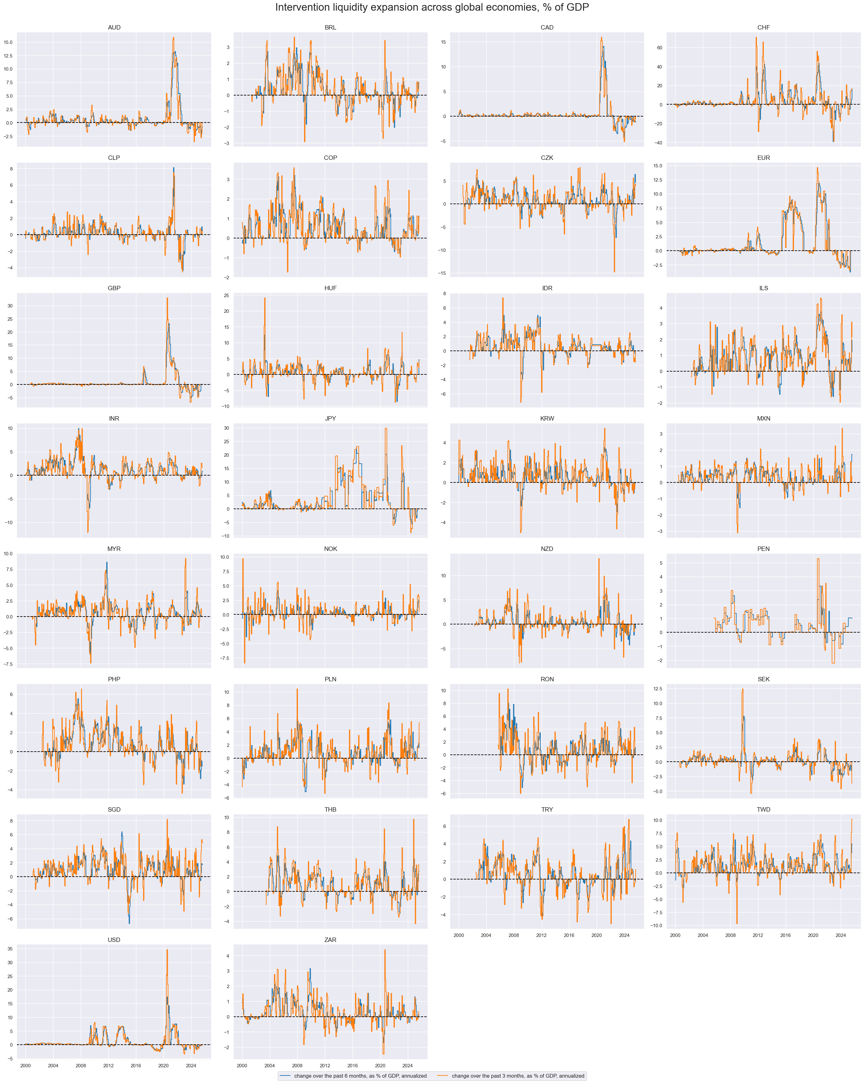
msp.view_timelines(
dfx,
xcats=xcatx[:2],
cids=cidx,
ncol=4,
start="2000-01-01",
size=(10, 5),
same_y=False,
title="Intervention liquidity expansion across global economies, % of GDP",
title_fontsize=24,
xcat_labels=dict_labs,
)
Global expansion rates #
# Global weighted composites of growth metrics

xcatx = cbal_dars + xcbal_dars

dict_globals = {
    "GLEQ": cids_eq,
    "DMEQ": cids_dmeq,
    "EMEQ": cids_emeq,
    "GLED": cids_eqdu,
    "DMED": cids_dmeqdu,
    "GLFX": cids_fx,
}

dfa = pd.DataFrame(columns=dfx.columns)

for k, v in dict_globals.items():
    for xc in xcatx:
        dfaa = msp.linear_composite(
            dfx,
            xcats=[xc],
            cids=v,
            weights="USDGDPWGT_SA_3YMA",  # USD GDP weights
            new_cid=k,
        )
        dfa = msm.update_df(dfa, dfaa)

dfx = msm.update_df(dfx, dfa)
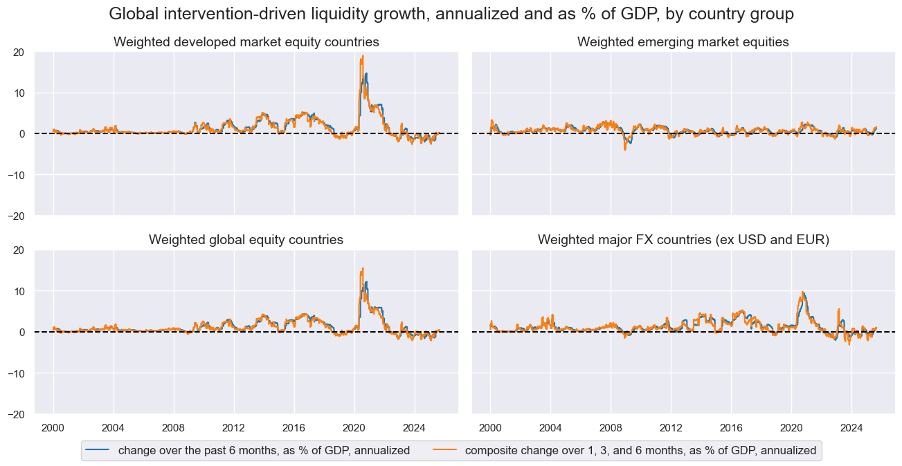
# Visualize new global aggregates

xcx = "INTLIQGDP_NSA"

dict_xcat_labs = {
    xcx + "_D1M1ML6AR": "change over the past 6 months, as % of GDP, annualized",
    xcx + "_D1M1ML3AR": "change over the past 3 months, as % of GDP, annualized",
    xcx + "_D1M1ML1AR": "change over the past 1 month, as % of GDP, annualized",
    xcx + "_DAR": "composite change over 1, 3, and 6 months, as % of GDP, annualized",
}
dict_cid_labs = {
    "GLEQ": "Weighted global equity countries",
    "DMEQ": "Weighted developed market equity countries",
    "EMEQ": "Weighted emerging market equities",
    "GLFX": "Weighted major FX countries (ex USD and EUR)",
}

allx = list(dict_xcat_labs.keys())
xcatx = [allx[i] for i in (0, 3)]
cidx = list(dict_cid_labs.keys())

msp.view_timelines(
    dfx,
    xcats=xcatx,
    cids=cidx,
    ncol=2,
    start="2000-01-01",
    aspect=2,
    height=2.2,
    title="Global intervention-driven liquidity growth, annualized and as % of GDP, by country group",
    xcat_labels=dict_xcat_labs,
    cid_labels=dict_cid_labs
)
Relative expansion rates #
Equity #
# Custom blacklist for equity

cidx = cids_eq
xcatx = ["EQXR_NSA"]

dfxx = dfx[dfx["xcat"].isin(xcatx) & dfx["cid"].isin(cidx)]
dfxx_m = (
    dfxx.groupby(["cid", "xcat"])
    .resample("M", on="real_date")
    .sum()["value"]
    .reset_index()
)

calcs = [f"EQ_BLACK = {xcatx[0]} / {xcatx[0]} - 1"] # returns zero if data present
dfa = msp.panel_calculator(dfxx_m, cids=cidx, calcs=calcs)
eq_black = msp.make_blacklist(dfa, "EQ_BLACK", nan_black=True) # blacklist if no data to avoid inclusion in relative basket calculations
# Relative values for equity markets

cidx = cids_eq
xcatx = cbal_dars + xcbal_dars

dfa = msp.make_relative_value(
    dfx,
    xcats=xcatx,
    cids=cidx,
    blacklist=eq_black,
    complete_cross=False,
    postfix="vGEQ",
)

dfx = msm.update_df(dfx, dfa)
Equity duration risk parity #
# Custom blacklist for equity duration

cidx = cids_eqdu
xcatx = ["EQXR_VT10", "DU05YXR_VT10"]

dfxx = dfx[dfx["xcat"].isin(xcatx) & dfx["cid"].isin(cidx)]

# use monthly resumplig to reduce calculation time for blacklist creation
dfxx_m = (
    dfxx.groupby(["cid", "xcat"])
    .resample("M", on="real_date")
    .sum()["value"]
    .reset_index()
)

calcs = [f"EQDU_BLACK = {xcatx[0]} / {xcatx[0]} + {xcatx[1]} / {xcatx[1]} - 2"] # returns zero if data present for both equity and duration returns
dfa = msp.panel_calculator(dfxx_m, cids=cidx, calcs=calcs)
eqdu_black = msp.make_blacklist(dfa, "EQDU_BLACK" ,nan_black=True)
eqdu_black
{'AUD': (Timestamp('1990-01-31 00:00:00'), Timestamp('2001-06-30 00:00:00')),
 'BRL': (Timestamp('1990-01-31 00:00:00'), Timestamp('2008-07-31 00:00:00')),
 'CAD': (Timestamp('1990-01-31 00:00:00'), Timestamp('1999-10-31 00:00:00')),
 'CHF': (Timestamp('1990-01-31 00:00:00'), Timestamp('1998-10-31 00:00:00')),
 'EUR': (Timestamp('1990-01-31 00:00:00'), Timestamp('1998-05-31 00:00:00')),
 'GBP': (Timestamp('1990-01-31 00:00:00'), Timestamp('1993-12-31 00:00:00')),
 'INR': (Timestamp('1990-01-31 00:00:00'), Timestamp('2006-04-30 00:00:00')),
 'KRW': (Timestamp('1990-01-31 00:00:00'), Timestamp('2006-04-30 00:00:00')),
 'MXN': (Timestamp('1990-01-31 00:00:00'), Timestamp('2005-12-31 00:00:00')),
 'MYR': (Timestamp('1990-01-31 00:00:00'), Timestamp('2005-12-31 00:00:00')),
 'PLN': (Timestamp('1990-01-31 00:00:00'), Timestamp('2013-08-31 00:00:00')),
 'SEK_1': (Timestamp('1990-01-31 00:00:00'), Timestamp('2005-01-31 00:00:00')),
 'SEK_2': (Timestamp('2008-04-30 00:00:00'), Timestamp('2008-05-31 00:00:00')),
 'SGD': (Timestamp('1990-01-31 00:00:00'), Timestamp('2006-04-30 00:00:00')),
 'THB': (Timestamp('1990-01-31 00:00:00'), Timestamp('2006-04-30 00:00:00')),
 'TRY': (Timestamp('1990-01-31 00:00:00'), Timestamp('2009-07-31 00:00:00')),
 'TWD': (Timestamp('1990-01-31 00:00:00'), Timestamp('2006-04-30 00:00:00')),
 'ZAR': (Timestamp('1990-01-31 00:00:00'), Timestamp('2001-05-31 00:00:00'))}
# Relative values for equity duration countries

cidx = cids_eqdu
xcatx = cbal_dars + xcbal_dars

dfa = msp.make_relative_value(
    dfx,
    xcats=xcatx,
    cids=cidx,
    blacklist=eqdu_black,
    complete_cross=False,
    postfix="vGED",
)

dfx = msm.update_df(dfx, dfa)
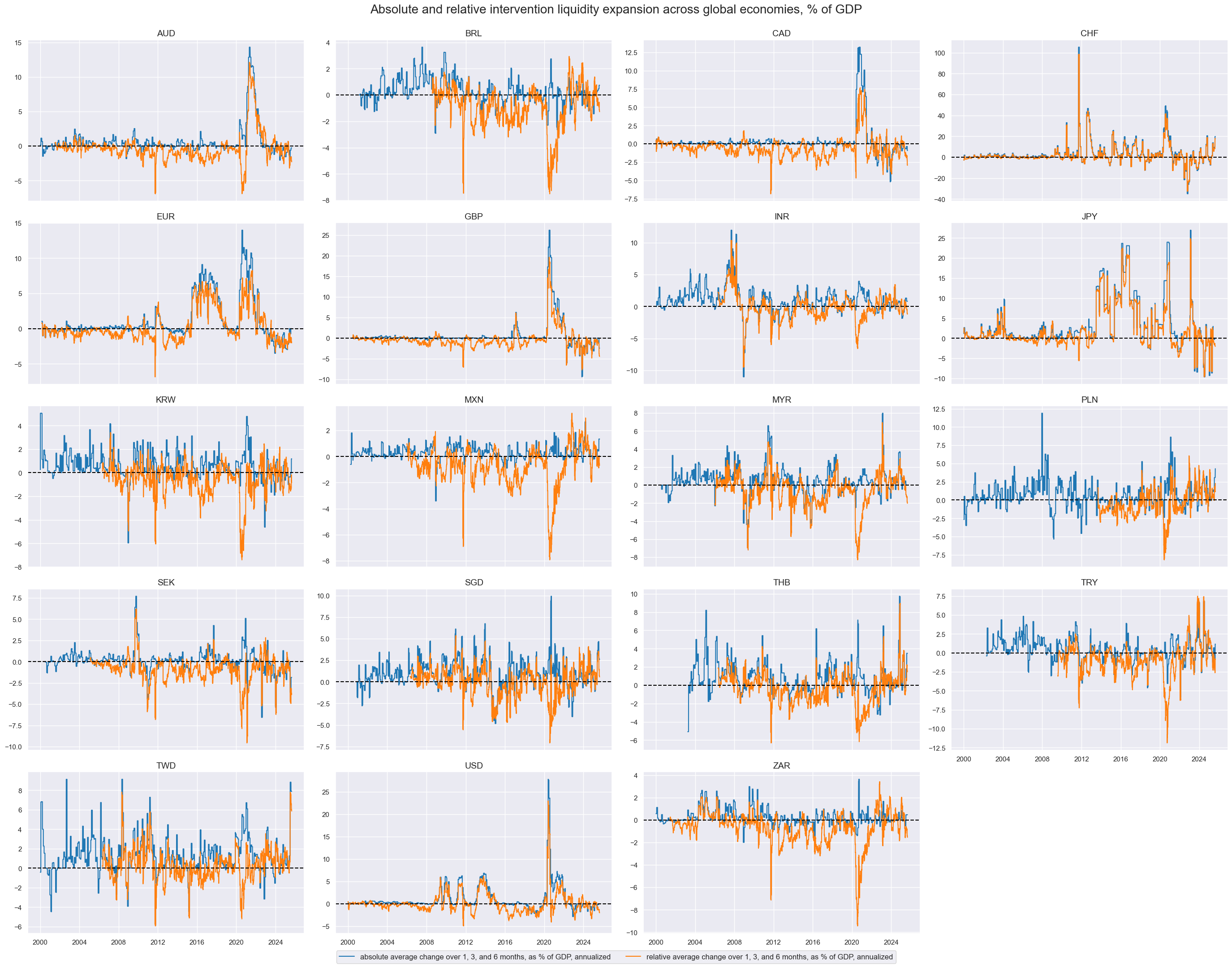
xcx = "INTLIQGDP_NSA"
dar = "DAR"

xcatx = [xcx + "_" + dar + pfix for pfix in ["", "vGED"]]
cidx = cids_eqdu

dict_xcat_labs = {
    xcx + "_" + dar: "absolute average change over 1, 3, and 6 months, as % of GDP, annualized",
    xcx + "_" + dar + "vGED": "relative average change over 1, 3, and 6 months, as % of GDP, annualized",
}

# visualize absolute and relative liquidity expansion rates. Note that relative expansion rates
# are only available for periods where both equity and duration returns are available due to blacklisting eqdu_black in previous cell

msp.view_timelines(
    dfx,
    xcats=xcatx,
    cids=cidx,
    ncol=4,
    start="2000-01-01",
    size=(10, 5),
    same_y=False,
    title="Absolute and relative intervention liquidity expansion across global economies, % of GDP",
    title_fontsize=20,
    xcat_labels=dict_xcat_labs,
)
FX #
# Relative values for FX countries

cidx = cids_fx
xcatx = cbal_dars + xcbal_dars

dfa = msp.make_relative_value(
    dfx,
    xcats=xcatx,
    cids=cidx,
    blacklist=fx_black,
    complete_cross=False,
    postfix="vGFX",
)

dfx = msm.update_df(dfx, dfa)
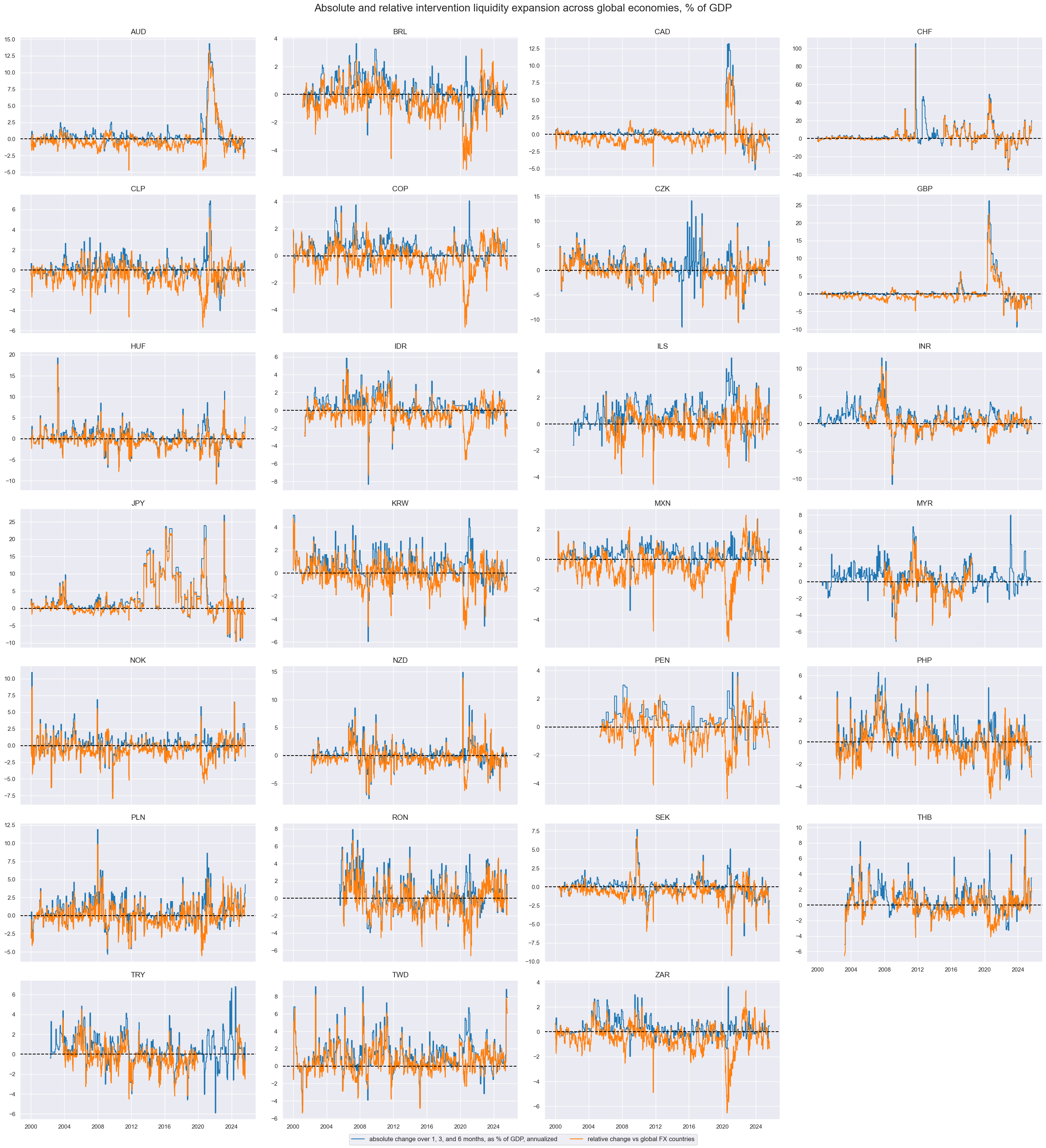
xcx = "INTLIQGDP_NSA"
dar = "DAR"

xcatx = [xcx + "_" + dar + pfix for pfix in ["", "vGFX"]]
cidx = cids_fx

dict_xcat_labs = {
    xcx + "_" + dar: "absolute change over 1, 3, and 6 months, as % of GDP, annualized",
    xcx + "_" + dar + "vGFX": "relative change vs global FX countries",
}

msp.view_timelines(
    dfx,
    xcats=xcatx,
    cids=cidx,
    ncol=4,
    start="2000-01-01",
    size=(10, 5),
    same_y=False,
    title="Absolute and relative intervention liquidity expansion across global economies, % of GDP",
    title_fontsize=20,
    xcat_labels=dict_xcat_labs,
)
Targets #
Directional #
# Risk parity returns

cidx = cids_eqdu

calc_edc = ["EQDUXR_RP = EQXR_VT10 + DU05YXR_VT10",
            "EQvDUXR_RP = EQXR_VT10 - DU05YXR_VT10"]

dfa = msp.panel_calculator(dfx, calcs=calc_edc, cids=cidx)
dfx = msm.update_df(dfx, dfa)

# Vol estimation of long-long risk parity positions

dfa = msp.historic_vol(
    dfx, xcat="EQDUXR_RP", cids=cidx, lback_meth="xma", postfix="_ASD"
)
dft = dfa.pivot(index="real_date", columns="cid", values="value")
dftx = dft.resample("BM").last().reindex(dft.index).ffill().shift(1)
dfax = dftx.unstack().reset_index().rename({0: "value"}, axis=1)
dfax["xcat"] = "EQDUXR_RP_ASDML1"
dfx = msm.update_df(dfx, dfax)

# Vol estimation of long-short risk parity positions

dfa = msp.historic_vol(
    dfx, xcat="EQvDUXR_RP", cids=cidx, lback_meth="xma", postfix="_ASD"
)
dft = dfa.pivot(index="real_date", columns="cid", values="value")
dftx = dft.resample("BM").last().reindex(dft.index).ffill().shift(1)
dfax = dftx.unstack().reset_index().rename({0: "value"}, axis=1)
dfax["xcat"] = "EQvDUXR_RP_ASDML1"
dfx = msm.update_df(dfx, dfax)

# Vol-target risk parity performance indicators

calc_vaj = [
    "EQDUXR_RPVT10 = 10 * EQDUXR_RP / EQDUXR_RP_ASDML1",
    "EQvDUXR_RPVT10 = 10 * EQvDUXR_RP / EQvDUXR_RP_ASDML1",
]
dfa = msp.panel_calculator(dfx, calcs=calc_vaj, cids=cidx)
dfx = msm.update_df(dfx, dfa)
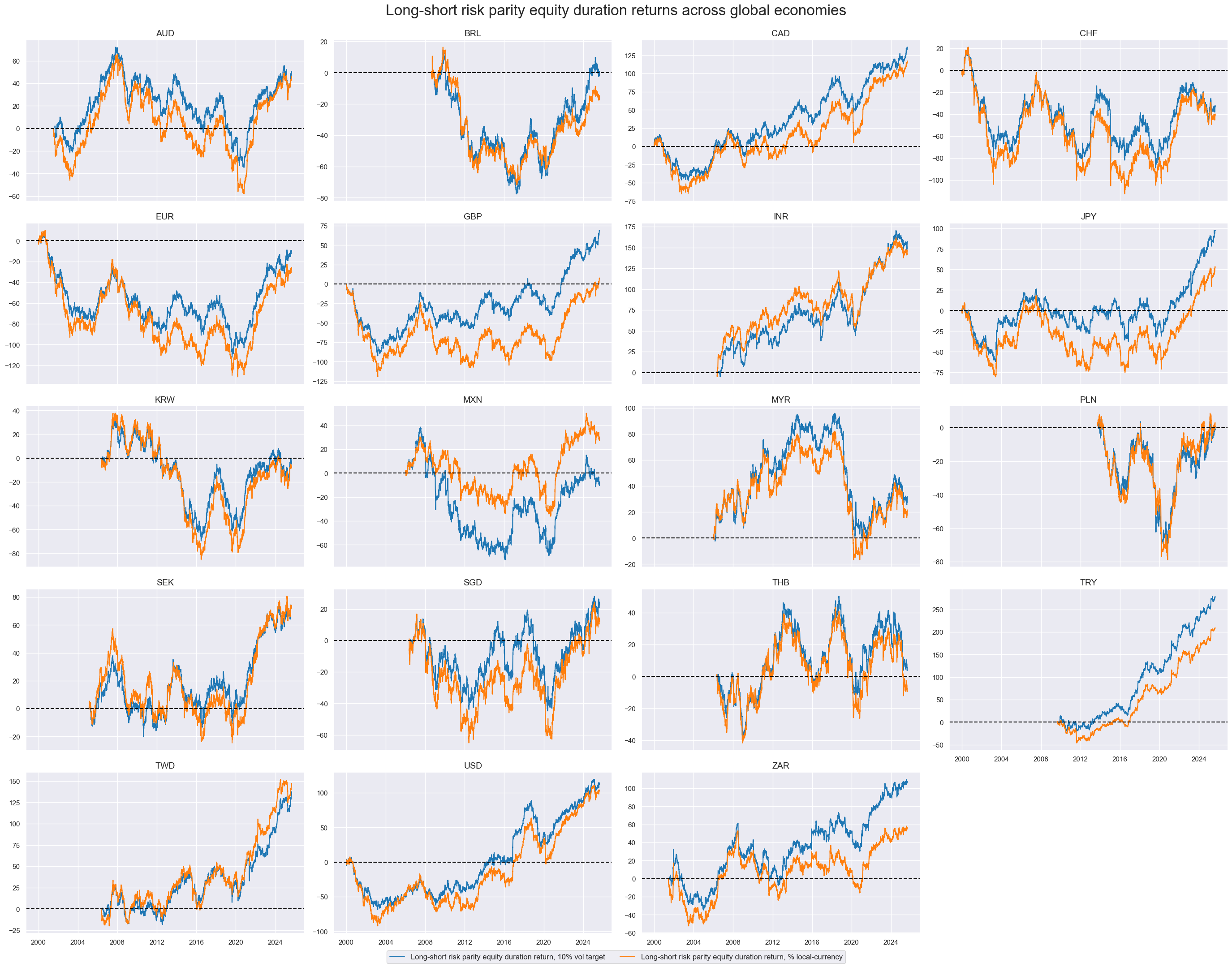
xcatx = ["EQvDUXR_RPVT10", "EQvDUXR_RP"]
cidx = cids_eqdu

dict_labs = {
    "EQvDUXR_RPVT10": "Long-short risk parity equity duration return, 10% vol target",
    "EQvDUXR_RP": "Long-short risk parity equity duration return, % local-currency",

}

msp.view_timelines(
    dfx,
    xcats=xcatx,
    cids=cidx,
    ncol=4,
    start="2000-01-01",
    size=(10, 5),
    cumsum=True,
    same_y=False,
    title="Long-short risk parity equity duration returns across global economies",
    xcat_labels=dict_labs,
    title_fontsize=24,
)
# Global basket proxy returns

dict_brets = {
    "GLEQ": [cids_eq, eq_black, ["EQXR_NSA", "EQXR_VT10"]],
    "DMEQ": [cids_dmeq, eq_black, ["EQXR_NSA", "EQXR_VT10"]],
    "EMEQ": [cids_emeq, eq_black, ["EQXR_NSA", "EQXR_VT10"]],
    "GLED": [cids_eqdu, eqdu_black, ["EQDUXR_RP", "EQDUXR_RPVT10", "EQvDUXR_RP", "EQvDUXR_RPVT10"]],
    "DMED": [cids_dmeqdu, eqdu_black, ["EQDUXR_RP", "EQDUXR_RPVT10", "EQvDUXR_RP", "EQvDUXR_RPVT10"]],
    "GLFX": [cids_fx, fx_black, ["FXXRHvGDRB_NSA", "FXXR_VT10"]],
}

dfa = pd.DataFrame(columns=dfx.columns)

for cid, params in dict_brets.items():
    cidx, black, xcatx = params
    for xc in xcatx:
        dfaa = msp.linear_composite(
            dfx,
            xcats=[xc],
            blacklist=black,
            cids=cidx,
            new_cid=cid,
        )
        dfa = msm.update_df(dfa, dfaa)

dfx = msm.update_df(dfx, dfa)

brets = [k + "_" + v[2][0] for k, v in dict_brets.items()]
brets_vt = [k + "_" + v[2][1] for k, v in dict_brets.items()]
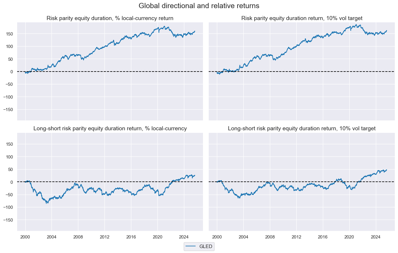
# Visualize new global aggregates

gcid = "GLED"
xcatx = dict_brets[gcid][2]

dict_xcat_labs = {
    "EQDUXR_RP": "Risk parity equity duration, % local-currency return",
    "EQDUXR_RPVT10": "Risk parity equity duration return, 10% vol target",
    "EQvDUXR_RP": "Long-short risk parity equity duration return, % local-currency",
    "EQvDUXR_RPVT10": "Long-short risk parity equity duration return, 10% vol target",
}


msp.view_timelines(
    dfx,
    xcats=xcatx,
    cids=[gcid],
    cumsum=True,
    xcat_grid=True,
    ncol=2,
    start="2000-01-01",
    size=(10, 5),
    xcat_labels=dict_xcat_labs,
    title="Global directional and relative returns",
)
Relative #
# Approximate relative vol-targeted returns

dict_rels = {
    "EQXR_VT10": [cids_eq, eq_black, "vGEQ"],
    "EQDUXR_RPVT10": [cids_eqdu, eqdu_black, "vGED"],
    "FXXR_VT10": [cids_fx, fx_black, "vGFX"],
}

dfa = pd.DataFrame(columns=list(dfx.columns))
for ret, params in dict_rels.items():
    cids_ac, blacklist, postfix = params
    dfaa = msp.make_relative_value(
        dfx, xcats=[ret], cids=cids_ac, postfix=postfix, blacklist=blacklist
    )
    dfa = msm.update_df(dfa, dfaa)

dfx = msm.update_df(dfx, dfa)

rels = [k + v[2] for k, v in dict_rels.items()]  # relative return categories
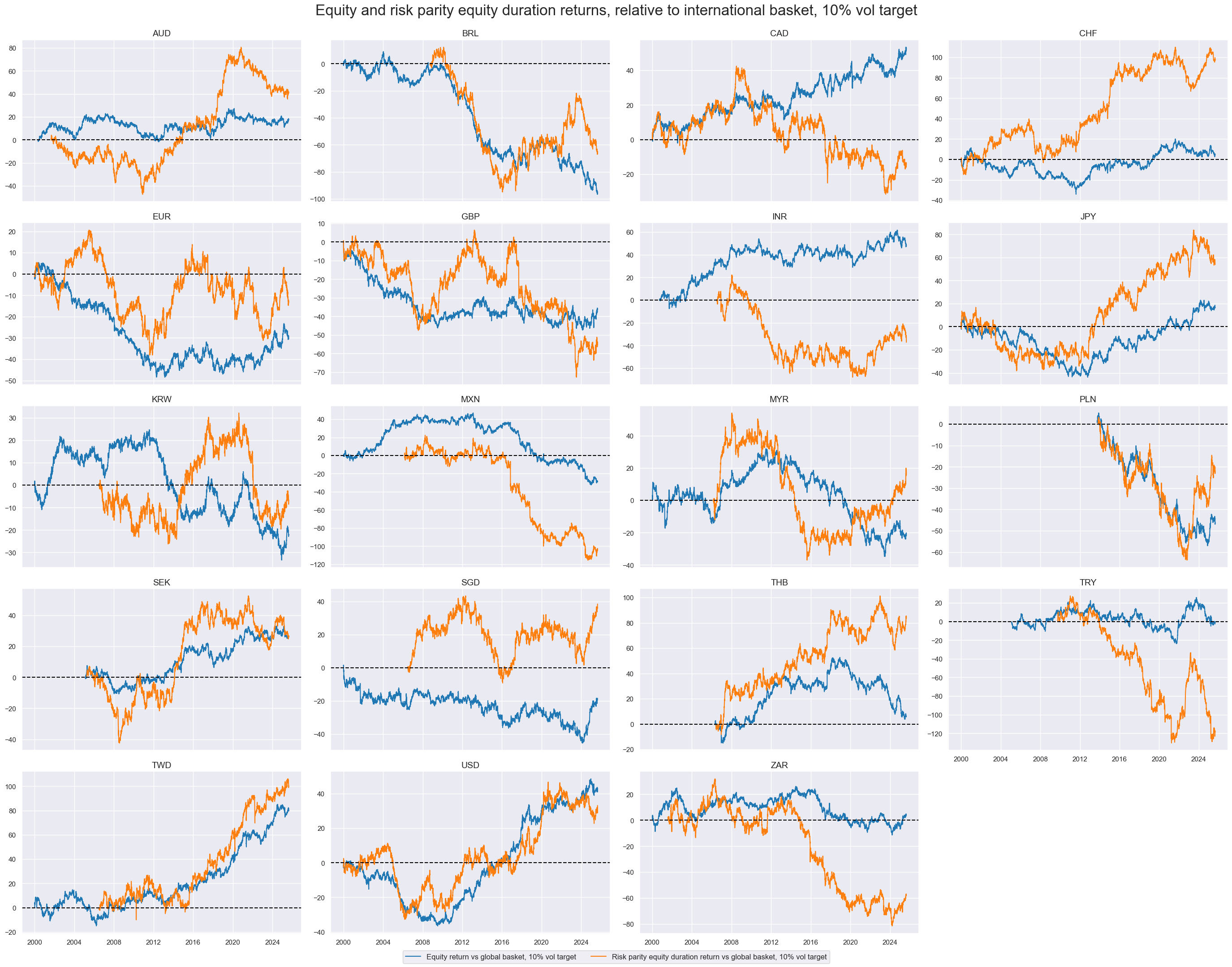
xcatx = ["EQXR_VT10vGEQ", "EQDUXR_RPVT10vGED"]
cidx = cids_eqdu

dict_xcat_labs = {
    "EQXR_VT10vGEQ": "Equity return vs global basket, 10% vol target",
    "EQDUXR_RPVT10vGED": "Risk parity equity duration return vs global basket, 10% vol target",

}

msp.view_timelines(
    dfx,
    xcats=xcatx,
    cids=cidx,
    cumsum=True,
    ncol=4,
    start="2000-01-01",
    size=(10, 5),
    same_y=False,
    title="Equity and risk parity equity duration returns, relative to international basket, 10% vol target",
    xcat_labels=dict_xcat_labs,
    title_fontsize=24,
)
Value checks #
Global equity strategy #
dict_eqd_glb = {
    "sigs": [
        "INTLIQGDP_NSA_DAR",
        "MBASEGDP_SA_DAR",
    ],
    "targ": "EQXR_NSA",
    "cids": ["GLEQ", "DMEQ"],
    "start": "2000-01-01",
    "black": eq_black,
    "crs": None,
    "srr": None,
    "pnls": None,
}
dix = dict_eqd_glb

sigx = dix["sigs"]
targx = dix["targ"]
cidx = dix["cids"]
start = dix["start"]

dict_cr = {}

for sig in sigx:
    for cid in cidx:
        lab = sig + "_" + cid
        dict_cr[lab] = msp.CategoryRelations(
            dfx,
            xcats=[sig, targx],
            cids=[cid],
            freq="M",
            lag=1,
            slip=1,
            blacklist=black,
            xcat_aggs=["last", "sum"],
            start=start,
        )
dix["crs"] = dict_cr
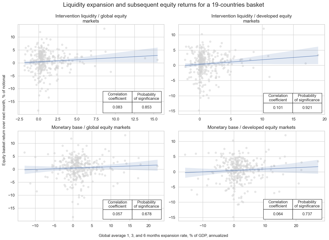
# Plotting panel scatters

dix = dict_eqd_glb
dict_cr = dix["crs"]

dict_eqd_glb_labs = {
    "INTLIQGDP_NSA_DAR_GLEQ": "Intervention liquidity / global equity markets",
    "INTLIQGDP_NSA_DAR_DMEQ": "Intervention liquidity / developed equity markets",
    "MBASEGDP_SA_DAR_GLEQ": "Monetary base / global equity markets",
    "MBASEGDP_SA_DAR_DMEQ": "Monetary base / developed equity markets",
}

keys   = list(dict_cr)
crs    = [dict_cr[k] for k in keys]
labels = [dict_eqd_glb_labs.get(k, k) for k in keys]

msv.multiple_reg_scatter(
    cat_rels=crs,
    ncol=2,
    nrow=2,
    figsize=(14, 10),
    title="Liquidity expansion and subsequent equity returns for a 19-countries basket",
    title_fontsize=18,
    xlab="Global average 1, 3, and 6 months expansion rate, % of GDP, annualized",
    ylab="Equity basket return over next month, % of notional",
    coef_box="lower right",
    prob_est="pool",
    share_axes=False,
    subplot_titles=labels,
)
dix = dict_eqd_glb

sigx = dix["sigs"]
targx = dix["targ"]
cidx = ['GLEQ']
start = dix["start"]

srr = mss.SignalReturnRelations(
    dfx,
    cids=cidx,
    sigs=sigx,
    rets=targx,
    freqs="M",
    start=start,
)

dix["srr"] = srr

display(srr.signals_table().sort_index().astype("float").round(3).T)
| Return | EQXR_NSA | |
|---|---|---|
| Signal | INTLIQGDP_NSA_DAR | MBASEGDP_SA_DAR |
| Frequency | M | M |
| Aggregation | last | last |
| accuracy | 0.593 | 0.524 |
| bal_accuracy | 0.551 | 0.484 |
| pos_sigr | 0.811 | 0.691 |
| pos_retr | 0.599 | 0.599 |
| pos_prec | 0.618 | 0.590 |
| neg_prec | 0.483 | 0.379 |
| pearson | 0.084 | 0.044 |
| pearson_pval | 0.144 | 0.440 |
| kendall | 0.026 | 0.004 |
| kendall_pval | 0.501 | 0.927 |
| auc | 0.532 | 0.486 |
# Simulate naive PnL

dix = dict_eqd_glb

sigx = dix["sigs"]
targx = dix["targ"]
cidx = ["GLEQ"]
start = dix["start"]

naive_pnl = msn.NaivePnL(
    dfx,
    ret=targx,
    sigs=sigx,
    cids=cidx,
    start=start,
    bms=["USD_EQXR_NSA", "USD_DU05YXR_NSA"],
)

for bias in [0, 1]:
    for sig in sigx:
        naive_pnl.make_pnl(
            sig,
            sig_add=bias,
            sig_op="zn_score_pan",
            thresh=4,
            rebal_freq="monthly",
            vol_scale=10,
            rebal_slip=1,
            pnl_name=sig + "_PZN" + str(bias),
        )

naive_pnl.make_long_pnl(label="Long only", vol_scale=10)
dix["pnls"] = naive_pnl
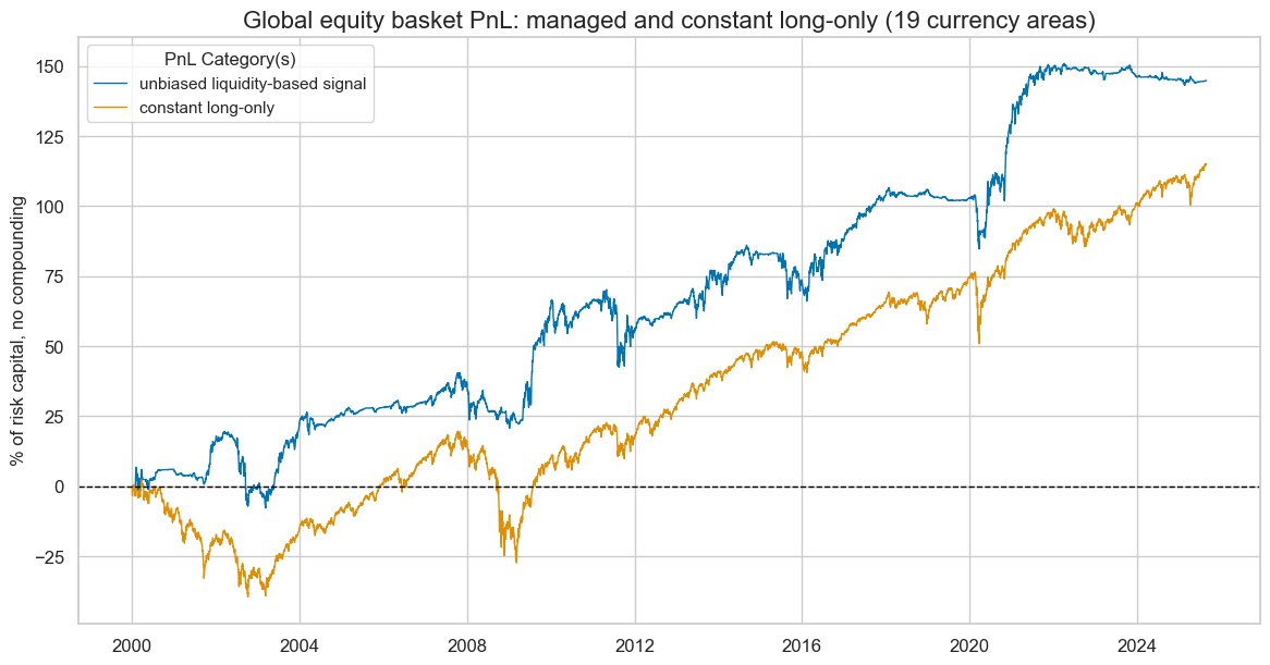
dix = dict_eqd_glb
sigx = 'INTLIQGDP_NSA_DAR'
targx = dix["targ"]
cidx = ["GLEQ"]
start = dix["start"]
naive_pnl = dix["pnls"]
pnls = [sigx + "_PZN0"] + ["Long only"]
naive_pnl.plot_pnls(
pnl_cats=pnls,
pnl_cids=["ALL"],
start=start,
title="Global equity basket PnL: managed and constant long-only (19 currency areas)",
title_fontsize=16,
figsize=(14, 7),
compounding=False,
xcat_labels= ["unbiased liquidity-based signal", "constant long-only"]
)
display(naive_pnl.evaluate_pnls(pnl_cats=pnls))
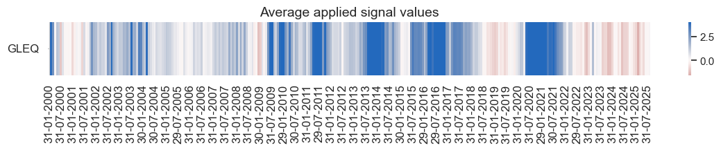
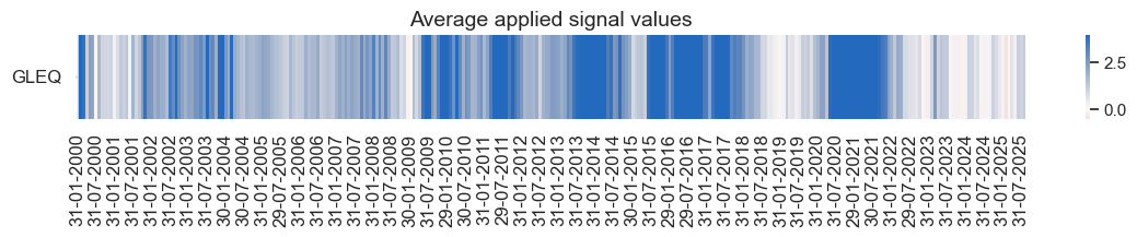
naive_pnl.signal_heatmap(
pnl_name=pnls[0],
freq="m",
start=start,
)
pnls = [sigx + "_PZN1"] + ["Long only"]
naive_pnl.plot_pnls(
pnl_cats=pnls,
pnl_cids=["ALL"],
start=start,
title="Global equity basket PnL: long-biased liquidity-based management and constant long-only (10% ar vol)",
title_fontsize=16,
figsize=(14, 7),
compounding=False,
xcat_labels=["long-biased liquidity-based signal", "constant long-only"]
)
display(naive_pnl.evaluate_pnls(pnl_cats=pnls))
naive_pnl.signal_heatmap(
pnl_name=pnls[0],
freq="m",
start=start,
)
| xcat | INTLIQGDP_NSA_DAR_PZN0 | Long only |
|---|---|---|
| Return % | 5.644726 | 4.485039 |
| St. Dev. % | 10.0 | 10.0 |
| Sharpe Ratio | 0.564473 | 0.448504 |
| Sortino Ratio | 0.796139 | 0.62179 |
| Max 21-Day Draw % | -22.767981 | -24.614661 |
| Max 6-Month Draw % | -26.237076 | -37.08632 |
| Peak to Trough Draw % | -27.632337 | -46.938297 |
| Top 5% Monthly PnL Share | 0.959228 | 0.754304 |
| USD_EQXR_NSA correl | 0.397344 | 0.936879 |
| USD_DU05YXR_NSA correl | -0.198423 | -0.257925 |
| Traded Months | 308 | 308 |
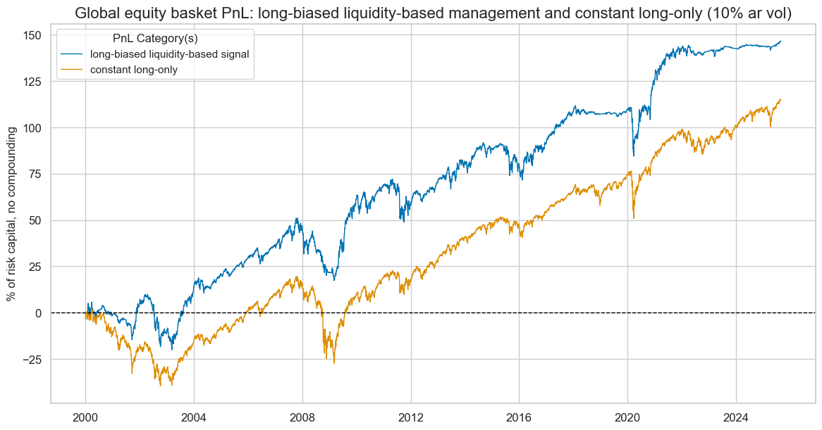
| xcat | INTLIQGDP_NSA_DAR_PZN1 | Long only |
|---|---|---|
| Return % | 5.708249 | 4.485039 |
| St. Dev. % | 10.0 | 10.0 |
| Sharpe Ratio | 0.570825 | 0.448504 |
| Sortino Ratio | 0.79534 | 0.62179 |
| Max 21-Day Draw % | -25.338329 | -24.614661 |
| Max 6-Month Draw % | -27.653099 | -37.08632 |
| Peak to Trough Draw % | -33.578172 | -46.938297 |
| Top 5% Monthly PnL Share | 0.814888 | 0.754304 |
| USD_EQXR_NSA correl | 0.535508 | 0.936879 |
| USD_DU05YXR_NSA correl | -0.232662 | -0.257925 |
| Traded Months | 308 | 308 |
Global long-short equity duration strategy #
dict_lsd_glb = {
    "sigs": [
        "INTLIQGDP_NSA_DAR",
        "MBASEGDP_SA_DAR",
    ],
    "targ": "EQvDUXR_RPVT10",
    "cids": ["GLED", "DMED"],
    "start": "2000-01-01",
    "black": eqdu_black,
    "crs": None,
    "srr": None,
    "pnls": None,
}
dix = dict_lsd_glb

sigx = dix["sigs"]
targx = dix["targ"]
cidx = dix["cids"]
start = dix["start"]
black = dix["black"]

dict_cr = {}

for sig in sigx:
    for cid in cidx:
        lab = sig + "_" + cid
        dict_cr[lab] = msp.CategoryRelations(
            dfx,
            xcats=[sig, targx],
            cids=[cid],
            freq="M",
            blacklist=black,
            lag=1,
            slip=1,
            xcat_aggs=["last", "sum"],
            start=start,
        )
dix["crs"] = dict_cr
# Plotting panel scatters
dix = dict_lsd_glb
dict_cr = dix["crs"]
dict_labs = {
"INTLIQGDP_NSA_DAR_GLED": "Intervention liquidity / global markets",
"INTLIQGDP_NSA_DAR_DMED": "Intervention liquidity / developed markets",
"MBASEGDP_SA_DAR_GLED": "Monetary base / global markets",
"MBASEGDP_SA_DAR_DMED": "Monetary base / developed markets",
}
crs = list(dict_cr.values())
crs_keys = list(dict_cr.keys())
labels = [dict_labs[key] for key in crs_keys]
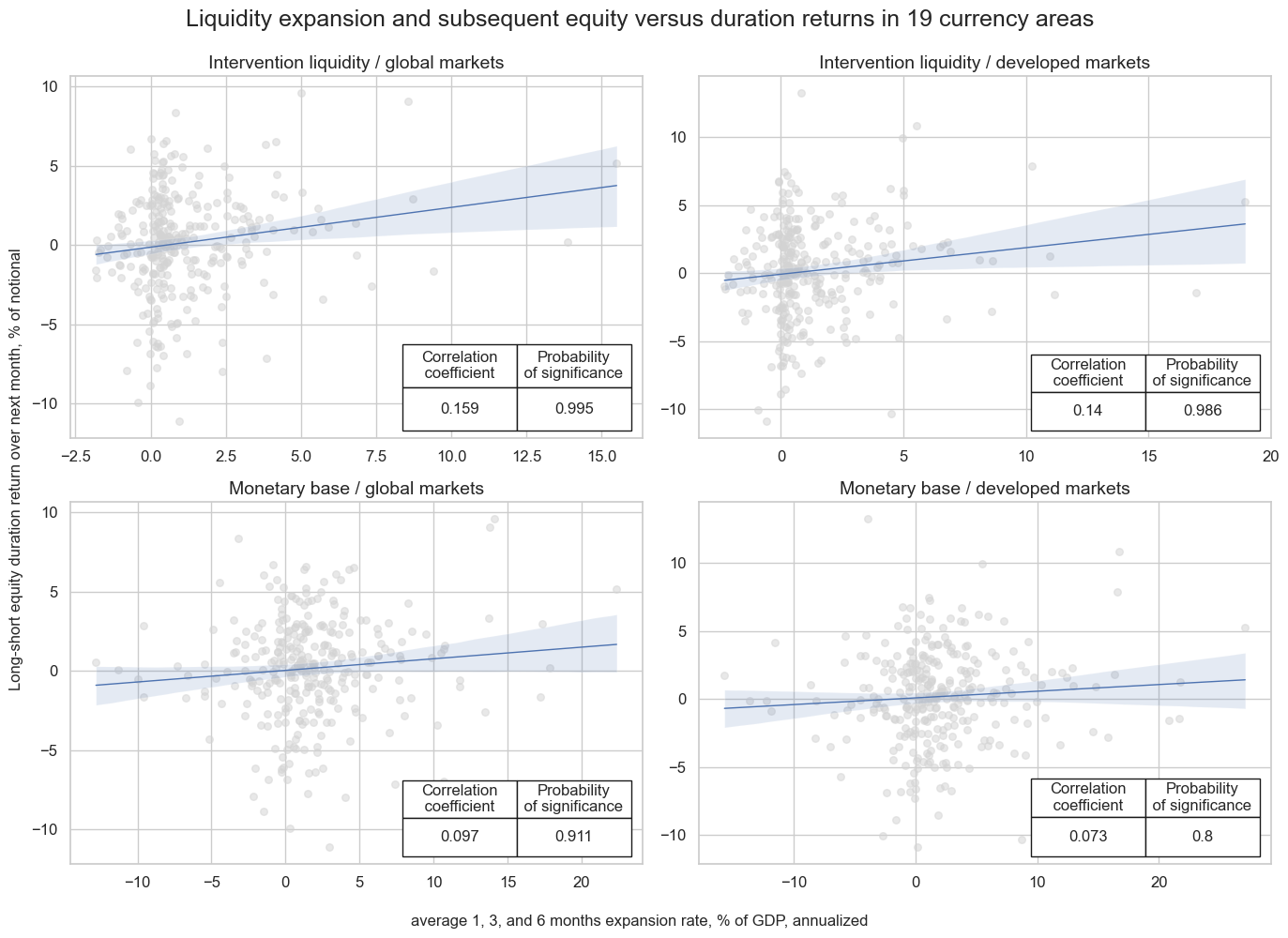
msv.multiple_reg_scatter(
cat_rels=crs,
ncol=2,
nrow=2,
figsize=(14, 10),
title="Liquidity expansion and subsequent equity versus duration returns in 19 currency areas",
title_fontsize=18,
xlab="average 1, 3, and 6 months expansion rate, % of GDP, annualized",
ylab="Long-short equity duration return over next month, % of notional",
coef_box="lower right",
prob_est="pool",
single_chart=True,
share_axes=False,
subplot_titles=labels,
)
dix = dict_lsd_glb

sigx = dix["sigs"]
targx = dix["targ"]
cidx = ['GLED']
start = dix["start"]

srr = mss.SignalReturnRelations(
    dfx,
    cids=cidx,
    sigs=sigx,
    rets=targx,
    freqs=["M"],
    start=start,
    blacklist=black,
)

display(srr.signals_table().sort_index().astype("float").round(3).T)

dix["srr"] = srr
| Return | EQvDUXR_RPVT10 | |
|---|---|---|
| Signal | INTLIQGDP_NSA_DAR | MBASEGDP_SA_DAR |
| Frequency | M | M |
| Aggregation | last | last |
| accuracy | 0.590 | 0.534 |
| bal_accuracy | 0.595 | 0.518 |
| pos_sigr | 0.811 | 0.691 |
| pos_retr | 0.550 | 0.550 |
| pos_prec | 0.586 | 0.561 |
| neg_prec | 0.603 | 0.474 |
| pearson | 0.154 | 0.090 |
| pearson_pval | 0.007 | 0.114 |
| kendall | 0.093 | 0.048 |
| kendall_pval | 0.015 | 0.208 |
| auc | 0.559 | 0.515 |
# Simulate naive PnL

dix = dict_lsd_glb

sigx = dix["sigs"]
targx = dix["targ"]
cidx = ["GLED"]
start = dix["start"]

naive_pnl = msn.NaivePnL(
    dfx,
    ret=targx,
    sigs=sigx,
    cids=cidx,
    start=start,
    bms=["USD_EQXR_NSA", "USD_DU05YXR_NSA"],
    blacklist=black
)

for bias in [0, 1]:
    for sig in sigx:
        naive_pnl.make_pnl(
            sig,
            sig_add=bias,
            sig_op="zn_score_pan",
            thresh=4,
            rebal_freq="weekly",
            neutral="zero",
            vol_scale=10,
            rebal_slip=1,
            pnl_name=sig + "_PZN" + str(bias),
        )

naive_pnl.make_long_pnl(label="Long only", vol_scale=10)
dix["pnls"] = naive_pnl
dix = dict_lsd_glb

sigx = 'INTLIQGDP_NSA_DAR'
targx = dix["targ"]
cidx = ["GLED"]
start = dix["start"]
naive_pnl = dix["pnls"]

pnls = [sigx + "_PZN0"] + ["Long only"]
naive_pnl.plot_pnls(
    pnl_cats=pnls,
    pnl_cids=["ALL"],
    start=start,
    title="Global long-short equity duration PnLs: managed and constant long-only (19 markets)",
    title_fontsize=16,
    figsize=(14, 7),
    compounding=False,
    xcat_labels= ["unbiased liquidity-based signals", "constant long-only"]
)

display(naive_pnl.evaluate_pnls(pnl_cats=pnls))
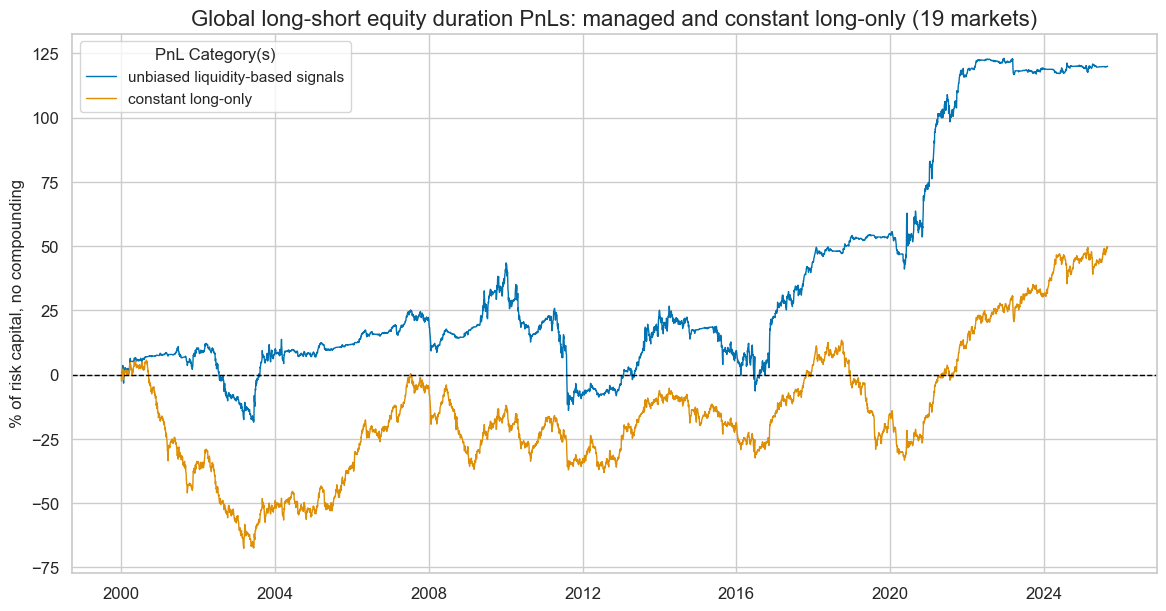
| xcat | INTLIQGDP_NSA_DAR_PZN0 | Long only |
|---|---|---|
| Return % | 4.683554 | 1.935181 |
| St. Dev. % | 10.0 | 10.0 |
| Sharpe Ratio | 0.468355 | 0.193518 |
| Sortino Ratio | 0.667744 | 0.266586 |
| Max 21-Day Draw % | -24.811886 | -14.862832 |
| Max 6-Month Draw % | -37.369212 | -29.955757 |
| Peak to Trough Draw % | -57.303965 | -73.19403 |
| Top 5% Monthly PnL Share | 1.159895 | 2.203486 |
| USD_EQXR_NSA correl | 0.28306 | 0.434215 |
| USD_DU05YXR_NSA correl | -0.314559 | -0.487182 |
| Traded Months | 308 | 308 |
Cross-country risk parity equity duration RV strategy #
dict_edr = {
    "sigs": [
        "INTLIQGDP_NSA_DARvGED",
        "XINTLIQGDP_NSA_DARvGED",
    ],
    "targ": "EQDUXR_RPVT10vGED",
    "cids": cids_eqdu,
    "start": "2000-01-01",
    "black": eqdu_black,
    "crs": None,
    "srr": None,
    "pnls": None,
}
dix = dict_edr

sigx = dix["sigs"]
targx = dix["targ"]
cidx = dix["cids"]
start = dix["start"]

dict_cr = {}

for sig in sigx:
    dict_cr[sig] = msp.CategoryRelations(
            dfx,
            xcats=[sig, targx],
            cids=cidx,
            freq="M",
            lag=1,
            slip=1,
            blacklist=black,
            xcat_aggs=["last", "sum"],
            start=start,
            xcat_trims=[30, 30],  # removes one vast outlier
        )

dix["crs"] = dict_cr
# Plotting panel scatters
dix = dict_edr
dict_cr = dix["crs"]
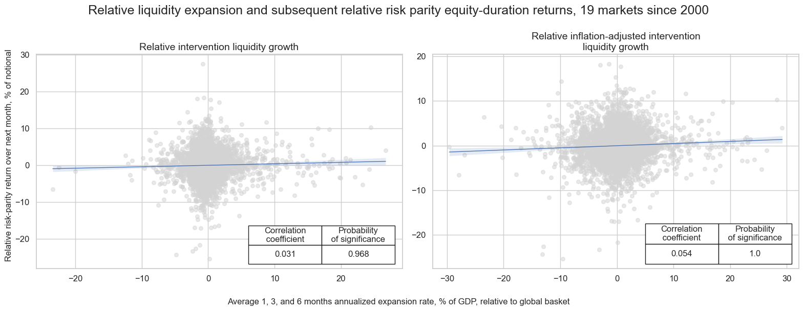
dict_edr_labs = {
"INTLIQGDP_NSA_DARvGED": "Relative intervention liquidity growth",
"XINTLIQGDP_NSA_DARvGED": "Relative inflation-adjusted intervention liquidity growth",
}
keys = list(dict_cr)
crs = [dict_cr[k] for k in keys]
labels = [dict_edr_labs.get(k, k) for k in keys]
msv.multiple_reg_scatter(
cat_rels=crs,
ncol=2,
nrow=1,
figsize=(16, 6),
title_fontsize=18,
title="Relative liquidity expansion and subsequent relative risk parity equity-duration returns, 19 markets since 2000",
xlab="Average 1, 3, and 6 months annualized expansion rate, % of GDP, relative to global basket",
ylab="Relative risk-parity return over next month, % of notional",
coef_box="lower right",
prob_est="map",
single_chart=True,
share_axes=False,
subplot_titles=labels,
)
dix = dict_edr

sigx = dix["sigs"]
targx = dix["targ"]
cidx = dix["cids"]
start = dix["start"]

srr = mss.SignalReturnRelations(
    dfx,
    cids=cidx,
    sigs=sigx,
    rets=targx,
    freqs="M",
    start=start,
)

display(srr.signals_table().sort_index().astype("float").round(3).T)

dix["srr"] = srr
| Return | EQDUXR_RPVT10vGED | |
|---|---|---|
| Signal | INTLIQGDP_NSA_DARvGED | XINTLIQGDP_NSA_DARvGED |
| Frequency | M | M |
| Aggregation | last | last |
| accuracy | 0.515 | 0.525 |
| bal_accuracy | 0.516 | 0.525 |
| pos_sigr | 0.382 | 0.523 |
| pos_retr | 0.497 | 0.497 |
| pos_prec | 0.516 | 0.521 |
| neg_prec | 0.515 | 0.529 |
| pearson | 0.033 | 0.052 |
| pearson_pval | 0.023 | 0.000 |
| kendall | 0.019 | 0.042 |
| kendall_pval | 0.044 | 0.000 |
| auc | 0.515 | 0.525 |
# Simulate naive PnL

dix = dict_edr

sigx = dix["sigs"]
targx = dix["targ"]
cidx = dix["cids"]
start = dix["start"]

naive_pnl = msn.NaivePnL(
    dfx,
    ret=targx,
    sigs=sigx,
    cids=cidx,
    start=start,
    bms=["USD_EQXR_NSA", "USD_DU05YXR_NSA"],
)

for sig in sigx:
    naive_pnl.make_pnl(
        sig,
        sig_add=bias,
        sig_op="zn_score_pan",
        thresh=4,
        rebal_freq="monthly",
        vol_scale=10,
        rebal_slip=1,
        pnl_name=sig + "_PZN",
    )

dix["pnls"] = naive_pnl
dix = dict_edr

sigx = dix["sigs"]
targx = dix["targ"]
cidx = dix["cids"]
start = dix["start"]
naive_pnl = dix["pnls"]

pnls = [sig + "_PZN" for sig in sigx]
pnl_labels={key + "_PZN": value for key, value in dict_edr_labs.items()}

naive_pnl.plot_pnls(
    pnl_cats=pnls,
    pnl_cids=["ALL"],
    start=start,
    title="Naive PnL of relative equity-duration risk parity strategies based on intervention liquidity growth (19 markets)",
    title_fontsize=16,
    figsize=(14, 7),
    compounding=False,
    xcat_labels=pnl_labels
)

display(naive_pnl.evaluate_pnls(pnl_cats=pnls))
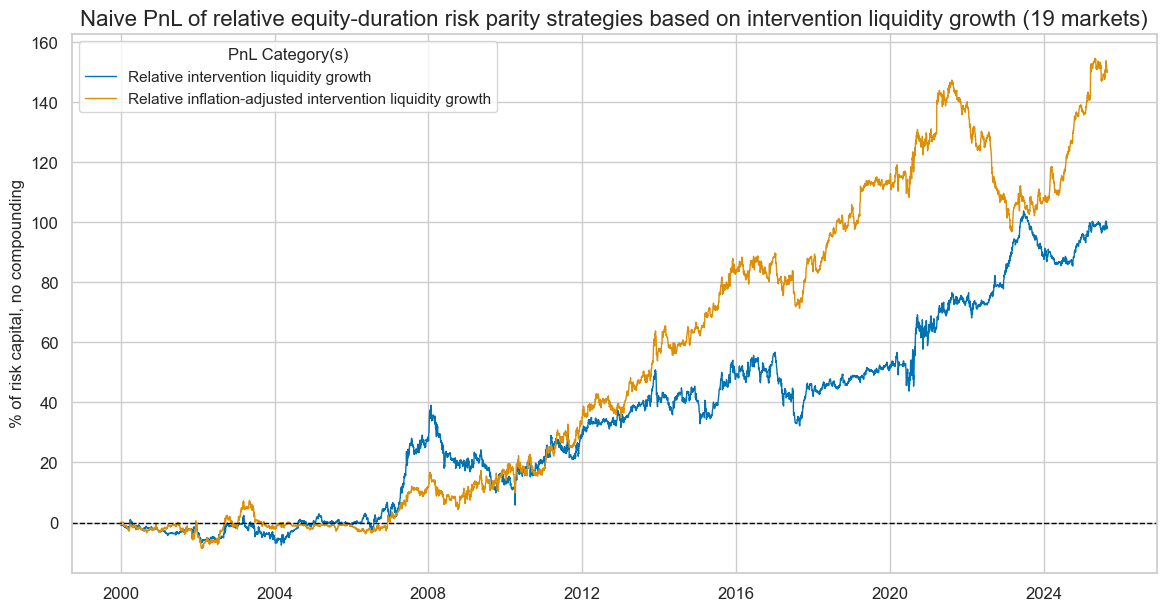
| xcat | INTLIQGDP_NSA_DARvGED_PZN | XINTLIQGDP_NSA_DARvGED_PZN |
|---|---|---|
| Return % | 3.845034 | 5.843183 |
| St. Dev. % | 10.0 | 10.0 |
| Sharpe Ratio | 0.384503 | 0.584318 |
| Sortino Ratio | 0.553761 | 0.872952 |
| Max 21-Day Draw % | -11.615999 | -14.879346 |
| Max 6-Month Draw % | -19.997573 | -28.116077 |
| Peak to Trough Draw % | -33.230382 | -50.485411 |
| Top 5% Monthly PnL Share | 0.931942 | 0.861858 |
| USD_EQXR_NSA correl | -0.040381 | -0.088306 |
| USD_DU05YXR_NSA correl | -0.02057 | 0.110234 |
| Traded Months | 308 | 308 |
Cross-country FX RV strategy #
dict_fxr = {
    "sigs": [
        "INTLIQGDP_NSA_DARvGFX",
        "XINTLIQGDP_NSA_DARvGFX",
    ],
    "targ": "FXXR_VT10vGFX",
    "cids": cids_fx,
    "start": "2000-01-01",
    "black": fx_black,
    "crs": None,
    "srr": None,
    "pnls": None,
}
dix = dict_fxr

sigx = dix["sigs"]
targx = dix["targ"]
cidx = dix["cids"]
start = dix["start"]
black = dix["black"]

dict_cr = {}

for sig in sigx:
    dict_cr[sig] = msp.CategoryRelations(
            dfx,
            xcats=[sig, targx],
            cids=cidx,
            freq="M",
            lag=1,
            slip=1,
            xcat_aggs=["last", "sum"],
            start=start,
            blacklist=black,
            xcat_trims=[30, 30],  # removes one vast outlier
        )

dix["crs"] = dict_cr
# Plotting panel scatters
dix = dict_fxr
dict_cr = dix["crs"]
crs = list(dict_cr.values())
crs_keys = list(dict_cr.keys())
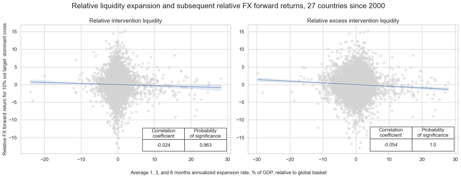
dict_fxr_labs = {
"INTLIQGDP_NSA_DARvGFX": "Relative intervention liquidity",
"XINTLIQGDP_NSA_DARvGFX": "Relative excess intervention liquidity",
}
keys = list(dict_cr)
crs = [dict_cr[k] for k in keys]
labels = [dict_fxr_labs.get(k, k) for k in keys]
msv.multiple_reg_scatter(
cat_rels=crs,
ncol=2,
nrow=1,
figsize=(16, 6),
title="Relative liquidity expansion and subsequent relative FX forward returns, 27 countries since 2000",
title_fontsize=18,
xlab="Average 1, 3, and 6 months annualized expansion rate, % of GDP, relative to global basket",
ylab="Relative FX forward return for 10% vol target: dominant cross",
coef_box="lower right",
prob_est="map",
share_axes=False,
subplot_titles=labels,
)
dix = dict_fxr

sigx = dix["sigs"]
targx = dix["targ"]
cidx = dix["cids"]
start = dix["start"]
black = dix["black"]

srr = mss.SignalReturnRelations(
    dfx,
    cids=cidx,
    sigs=sigx,
    sig_neg=[True]*len(sigx),
    blacklist=black,
    rets=targx,
    freqs="M",
    start=start,
)

display(srr.signals_table().sort_index().astype("float").round(3).T)

dix["srr"] = srr
| Return | FXXR_VT10vGFX | |
|---|---|---|
| Signal | INTLIQGDP_NSA_DARvGFX_NEG | XINTLIQGDP_NSA_DARvGFX_NEG |
| Frequency | M | M |
| Aggregation | last | last |
| accuracy | 0.502 | 0.523 |
| bal_accuracy | 0.501 | 0.524 |
| pos_sigr | 0.593 | 0.469 |
| pos_retr | 0.509 | 0.508 |
| pos_prec | 0.510 | 0.533 |
| neg_prec | 0.491 | 0.514 |
| pearson | 0.026 | 0.052 |
| pearson_pval | 0.027 | 0.000 |
| kendall | 0.010 | 0.036 |
| kendall_pval | 0.186 | 0.000 |
| auc | 0.501 | 0.524 |
# Simulate naive PnL

dix = dict_fxr

sigx = dix["sigs"]
targx = dix["targ"]
cidx = dix["cids"]
start = dix["start"]

naive_pnl = msn.NaivePnL(
    dfx,
    ret=targx,
    sigs=sigx,
    cids=cidx,
    start=start,
    bms=["USD_EQXR_NSA", "USD_DU05YXR_NSA"],
)

for sig in sigx:
    naive_pnl.make_pnl(
        sig,
        sig_neg=True,
        sig_op="zn_score_pan",
        thresh=4,
        rebal_freq="monthly",
        vol_scale=10,
        rebal_slip=1,
        pnl_name=sig + "_PZN",
    )

dix["pnls"] = naive_pnl
dix = dict_fxr

sigx = dix["sigs"]
targx = dix["targ"]
cidx = dix["cids"]
start = dix["start"]
naive_pnl = dix["pnls"]

pnls = [sig + "_PZN" for sig in sigx]
pnl_labels={key + "_PZN": value for key, value in dict_fxr_labs.items()}

naive_pnl.plot_pnls(
    pnl_cats=pnls,
    pnl_cids=["ALL"],
    start=start,
    title="Naive PnL of relative FX forward strategies based on intervention liquidity growth (27 currencies)",
    title_fontsize=16,
    figsize=(14, 7),
    compounding=False,
    xcat_labels=pnl_labels
)

df_eval = naive_pnl.evaluate_pnls(pnl_cats = pnls, start = start)
df_eval = df_eval.rename (columns = pnl_labels)
display(df_eval.astype("float").round(2))
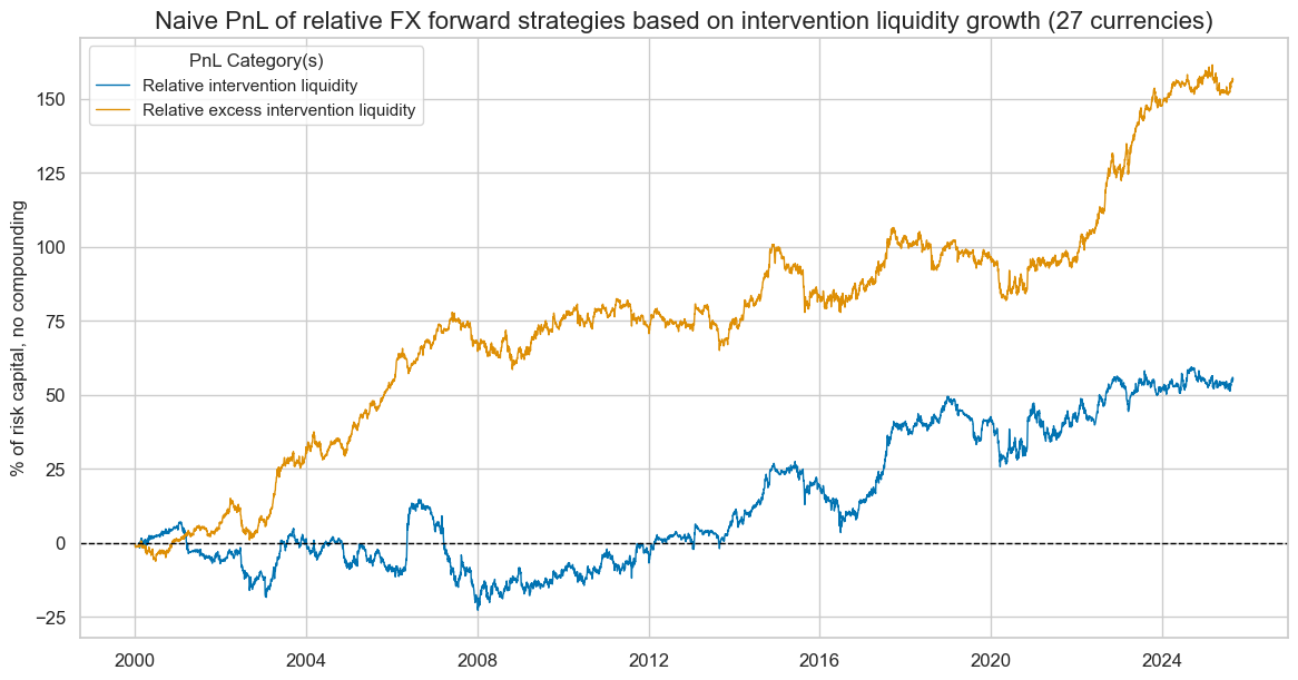
| xcat | Relative intervention liquidity | Relative excess intervention liquidity |
|---|---|---|
| Return % | 2.15 | 6.10 |
| St. Dev. % | 10.00 | 10.00 |
| Sharpe Ratio | 0.21 | 0.61 |
| Sortino Ratio | 0.31 | 0.87 |
| Max 21-Day Draw % | -12.80 | -13.16 |
| Max 6-Month Draw % | -22.25 | -17.83 |
| Peak to Trough Draw % | -37.46 | -24.61 |
| Top 5% Monthly PnL Share | 2.05 | 0.67 |
| USD_EQXR_NSA correl | 0.11 | 0.19 |
| USD_DU05YXR_NSA correl | -0.06 | -0.13 |
| Traded Months | 308.00 | 308.00 |
Strategy portfolio PnL #
all_naive_pnls = {}
all_naive_pnl_names = {}
# Global equity directional

dix = dict_eqd_glb

sig = "INTLIQGDP_NSA_DAR"
targx = dix["targ"]
cidx = "GLEQ"
start = dix["start"]
black = dix["black"]

pnl_name = sig + "_EQD"

naive_pnl = msn.NaivePnL(
    dfx,
    ret=targx,
    sigs=[sig],
    cids=[cidx],
    start=start,
    blacklist=black
)

naive_pnl.make_pnl(
    sig,
    sig_op="zn_score_pan",
    thresh=4,
    rebal_freq="monthly",
    vol_scale=None,
    rebal_slip=1,
    pnl_name=pnl_name,
    leverage=1/2,
)

naive_pnl.plot_pnls(
    pnl_cats=[pnl_name],
    start=start,
    figsize=(16, 8),
    title = "Global equity PnL: liquidity-based management",
    xcat_labels=["average 1, 3, and 6 months expansion rate, % of GDP, annualized"]
)

display(naive_pnl.evaluate_pnls(pnl_cats=[pnl_name]))

all_naive_pnls[pnl_name] = naive_pnl
all_naive_pnl_names[pnl_name] = pnl_name
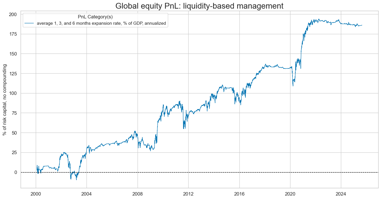
| xcat | INTLIQGDP_NSA_DAR_EQD |
|---|---|
| Return % | 7.276389 |
| St. Dev. % | 12.860087 |
| Sharpe Ratio | 0.565812 |
| Sortino Ratio | 0.798028 |
| Max 21-Day Draw % | -29.231792 |
| Max 6-Month Draw % | -33.685761 |
| Peak to Trough Draw % | -35.477136 |
| Top 5% Monthly PnL Share | 0.958539 |
| Traded Months | 307 |
# Global long-short equity-duration

dix = dict_lsd_glb

sigx = "INTLIQGDP_NSA_DAR"
targx = dix["targ"]
cidx = "GLED"
start = dix["start"]
black = dix["black"]

pnl_name = sig + "_LSD"

naive_pnl = msn.NaivePnL(
    dfx,
    ret=targx,
    sigs=[sigx],
    cids=[cidx],
    start=start,
    blacklist=black,
)

naive_pnl.make_pnl(
    sigx,
    sig_op="zn_score_pan",
    thresh=4,
    rebal_freq="monthly",
    vol_scale=None,
    rebal_slip=1,
    pnl_name=pnl_name,
    leverage=1/2,
)

naive_pnl.plot_pnls(
    pnl_cats=[pnl_name],
    start=start,
    title="Global long-short equity duration PnL: liquidity-based management",
    xcat_labels=["average 1, 3, and 6 months liquidity expansion rate, % of GDP, annualized"],
    figsize=(16, 8),
)

display(naive_pnl.evaluate_pnls(pnl_cats=[pnl_name]))

all_naive_pnls[pnl_name] = naive_pnl
all_naive_pnl_names[pnl_name] = pnl_name
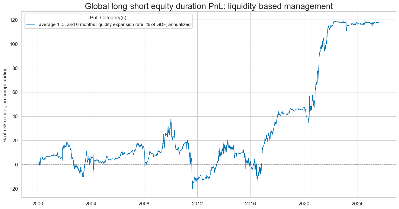
| xcat | INTLIQGDP_NSA_DAR_LSD |
|---|---|
| Return % | 4.610953 |
| St. Dev. % | 10.319443 |
| Sharpe Ratio | 0.446822 |
| Sortino Ratio | 0.633024 |
| Max 21-Day Draw % | -25.386848 |
| Max 6-Month Draw % | -37.24852 |
| Peak to Trough Draw % | -58.099965 |
| Top 5% Monthly PnL Share | 1.224703 |
| Traded Months | 307 |
# Relative risk parity

dix = dict_edr

sigx = "XINTLIQGDP_NSA_DARvGEQ"
targx = dix["targ"]
cidx = dix["cids"]
start = dix["start"]
black = dix["black"]

pnl_name = sigx + "_EDR"

naive_pnl = msn.NaivePnL(
    dfx,
    ret=targx,
    sigs=[sigx],
    cids=cidx,
    start=start,
    blacklist=black
)

naive_pnl.make_pnl(
    sigx,
    sig_op="zn_score_pan",
    thresh=4,
    rebal_freq="monthly",
    vol_scale=None,
    rebal_slip=1,
    pnl_name=pnl_name,
    leverage=1/8,
)

naive_pnl.plot_pnls(
    pnl_cats=[pnl_name],
    start=start,
    figsize=(16, 8),
    title = "Cross-country risk parity equity duration RV strategy: excess liquidity-based management",
    xcat_labels=["average 1, 3, and 6 months excess expansion rate, % of GDP, annualized, relative to global equity duration basket"]
)

display(naive_pnl.evaluate_pnls(pnl_cats=[pnl_name]))

all_naive_pnls[pnl_name] = naive_pnl
all_naive_pnl_names[pnl_name] = pnl_name
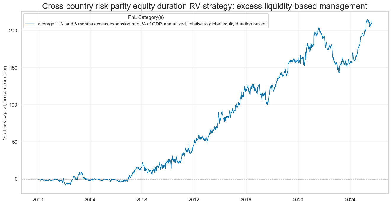
| xcat | XINTLIQGDP_NSA_DARvGEQ_EDR |
|---|---|
| Return % | 8.138201 |
| St. Dev. % | 13.525144 |
| Sharpe Ratio | 0.601709 |
| Sortino Ratio | 0.894373 |
| Max 21-Day Draw % | -17.224973 |
| Max 6-Month Draw % | -33.486371 |
| Peak to Trough Draw % | -61.860319 |
| Top 5% Monthly PnL Share | 0.821141 |
| Traded Months | 308 |
# Relative FX

dix = dict_fxr

sigx = "XINTLIQGDP_NSA_DARvGFX"
targx = dix["targ"]
cidx = dix["cids"]
start = dix["start"]
black = dix["black"]

pnl_name = sigx + "_FXR"

naive_pnl = msn.NaivePnL(
    dfx,
    ret=targx,
    sigs=[sigx],
    cids=cidx,
    start=start,
    blacklist=black
)

naive_pnl.make_pnl(
    sigx,
    sig_op="zn_score_pan",
    sig_neg=True,
    thresh=4,
    rebal_freq="monthly",
    vol_scale=None,
    rebal_slip=1,
    pnl_name=pnl_name,
    leverage=1/8,
)

naive_pnl.plot_pnls(
    pnl_cats=[pnl_name],
    start=start,
    figsize=(16, 8),
    title = "Cross-country FX RV PnL: excess liquidity-based management",
    xcat_labels=["average 1, 3, and 6 months excess expansion rate, % of GDP, annualized"]
)

display(naive_pnl.evaluate_pnls(pnl_cats=[pnl_name]))

all_naive_pnls[pnl_name] = naive_pnl
all_naive_pnl_names[pnl_name] = pnl_name
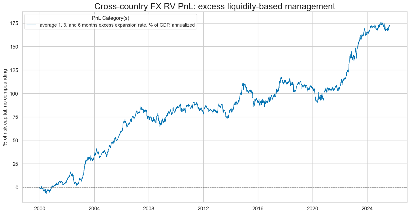
| xcat | XINTLIQGDP_NSA_DARvGFX_FXR |
|---|---|
| Return % | 6.720861 |
| St. Dev. % | 11.018189 |
| Sharpe Ratio | 0.609979 |
| Sortino Ratio | 0.866406 |
| Max 21-Day Draw % | -14.499917 |
| Max 6-Month Draw % | -19.64852 |
| Peak to Trough Draw % | -27.118017 |
| Top 5% Monthly PnL Share | 0.670378 |
| Traded Months | 308 |
# Combine PnL data into a single quantamental dataframe

unit_pnl_name = "PNLx"

df_pnls = QuantamentalDataFrame.from_qdf_list(
    [
        QuantamentalDataFrame.from_long_df(
            df=pnl.df[
                (pnl.df["xcat"] == all_naive_pnl_names[key]) & (pnl.df["cid"] == "ALL")
            ],
            cid=key[-3:],
            xcat=unit_pnl_name,
        )
        for key, pnl in all_naive_pnls.items()
    ]
)
# Create a wide dataframe of equal signals for each strategy

sig_value = 1
usig = "USIG"  # unit signal name
pnl_names=[pnl[-3:] for pnl in all_naive_pnls.keys()]

dt_range = pd.bdate_range(start=dfx["real_date"].min(), end=dfx["real_date"].max())
df_usigs = pd.DataFrame(
    data=sig_value, columns=pnl_names, index=dt_range
)
df_usigs.index.name = "real_date"
df_usigs.columns += f"_{usig}"
# Concat the unit signals to the PNL dataframe

df_usigs = msm.utils.ticker_df_to_qdf(df_usigs)
df_pnls = msm.update_df(df_pnls, df_usigs)
dfx = msm.update_df(dfx, df_pnls)
# Calculate the combined PnL

all_pnl = msn.NaivePnL(
    dfx,
    ret=unit_pnl_name,  # return on USD1 invested in strategy identified by cid
    sigs=[usig],
    cids=pnl_names,
    start="2000-01-01",
    bms=["USD_EQXR_NSA", "USD_DU05YXR_NSA"],
)
all_pnl.make_pnl(sig=usig, sig_op="raw", leverage=1/4)

all_pnl.plot_pnls(
    pnl_cats=[f"PNL_{usig}"],
    start="2000-01-01",
    title="Naive PnL of portfolio of two directional and two relative value liquidity strategies",
    title_fontsize=16,
    figsize=(13, 7),
    xcat_labels=["equal-weighted portfolio of four liquidity-based strategies"],
)
display(all_pnl.evaluate_pnls(pnl_cats=[f"PNL_{usig}"]))
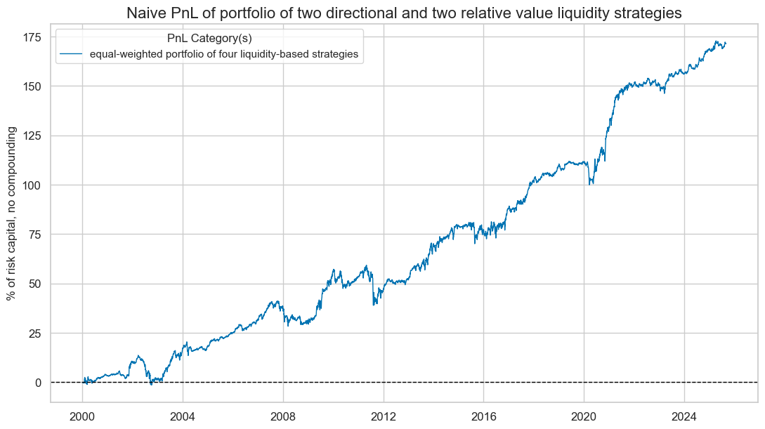
| xcat | PNL_USIG |
|---|---|
| Return % | 6.684836 |
| St. Dev. % | 7.10953 |
| Sharpe Ratio | 0.940264 |
| Sortino Ratio | 1.346988 |
| Max 21-Day Draw % | -15.545279 |
| Max 6-Month Draw % | -18.349746 |
| Peak to Trough Draw % | -20.328798 |
| Top 5% Monthly PnL Share | 0.526469 |
| USD_EQXR_NSA correl | 0.313906 |
| USD_DU05YXR_NSA correl | -0.209756 |
| Traded Months | 308 |
# Calculate the combined PnL

all_pnl = msn.NaivePnL(
    dfx,
    ret=unit_pnl_name,  # return on USD1 invested in strategy identified by cid
    sigs=[usig],
    cids=['EDR', 'FXR'],
    start="2000-01-01",
    bms=["USD_EQXR_NSA", "USD_DU05YXR_NSA"],
)
all_pnl.make_pnl(sig=usig, sig_op="raw", leverage=1/4)

all_pnl.plot_pnls(
    pnl_cats=[f"PNL_{usig}"],
    start="2000-01-01",
    title="PnL contributions of two liquidity-based relative value strategies (before transaction costs)",
    title_fontsize=16,
    figsize=(13, 7),
    xcat_labels=["equal-weighted portfolio of two RV liquidity-based strategies"],
)
display(all_pnl.evaluate_pnls(pnl_cats=[f"PNL_{usig}"]))
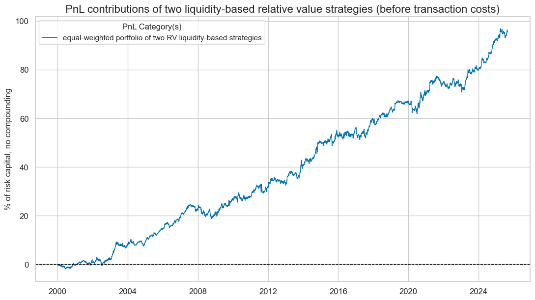
| xcat | PNL_USIG |
|---|---|
| Return % | 3.721442 |
| St. Dev. % | 3.992012 |
| Sharpe Ratio | 0.932222 |
| Sortino Ratio | 1.389845 |
| Max 21-Day Draw % | -4.316946 |
| Max 6-Month Draw % | -5.546541 |
| Peak to Trough Draw % | -6.62389 |
| Top 5% Monthly PnL Share | 0.48664 |
| USD_EQXR_NSA correl | 0.054717 |
| USD_DU05YXR_NSA correl | -0.005626 |
| Traded Months | 308 |