U.S. special data surprises #
This category group contains economic surprise indicators specific to the US. Economic surprises are deviations of point-in-time quantamental indicators from predicted values. For an in-depth explanation, please read Appendix 2 .
Business surveys #
Ticker : ISMMANU_SA_3MMA_ARMAS / ISMMANU_SA_D3M3ML3_ARMAS
Label : ISM manufacturing survey, sa, ARMA(1,1)-based surprises: 3mma / diff 3m/3m
Definition : ISM manufacturing survey headline index, seasonally adjusted, ARMA(1,1)-based surprises: 3 month moving average / difference of latest 3 months over previous 3 months
Notes :
-
Refer to the section on US Buisness surveys for notes on the underlying data series.
-
Expected values for release dates are based on an “ARMA(1,1)” model. This is a simple univariate time series model that predicts increments based on an autoregressive component, i.e., last period’s value, and a moving average component, represented by last period’s error. The coefficients of the model are estimated sequentially based on the vintages of production indices. And each vintage-specific model produces a one-step-ahead forecast for the subsequent observation period.
Ticker : ISMSERV_SA_3MMA_ARMAS / ISMSERV_SA_D3M3ML3_ARMAS
Label : ISM services survey, sa, ARMA(1,1)-based surprises: 3mma / diff 3m/3m
Definition : ISM services survey headline index, seasonally adjusted, ARMA(1,1)-based surprises: 3 month moving average / difference of latest 3 months over previous 3 months
Notes :
-
Refer to the section on US Buisness surveys for notes on the underlying data series.
-
Expected values for release dates are based on an “ARMA(1,1)” model. This is a simple univariate time series model that predicts increments based on an autoregressive component, i.e., last period’s value, and a moving average component, represented by last period’s error. The coefficients of the model are estimated sequentially based on the vintages of production indices. And each vintage-specific model produces a one-step-ahead forecast for the subsequent observation period.
Ticker : PHILMANU_SA_3MMA_ARMAS / PHILMANU_SA_D3M3ML3_ARMAS
Label : Philadelphia manufacturing survey, sa, ARMA(1,1)-based surprises: 3mma / diff 3m/3m
Definition : Federal Reserve Bank of Philadelphia manufacturing survey, general activity, seasonally adjusted, ARMA(1,1)-based surprises: 3 month moving average / difference of latest 3 months over previous 3 months
Notes :
-
Refer to the section on US Buisness surveys for notes on the underlying data series.
-
Expected values for release dates are based on an “ARMA(1,1)” model. This is a simple univariate time series model that predicts increments based on an autoregressive component, i.e., last period’s value, and a moving average component, represented by last period’s error. The coefficients of the model are estimated sequentially based on the vintages of production indices. And each vintage-specific model produces a one-step-ahead forecast for the subsequent observation period.
Ticker : NYMANU_SA_3MMA_ARMAS / NYMANU_SA_D3M3ML3_ARMAS
Label : Empire State manufacturing survey, sa, ARMA(1,1)-based surprises: 3mma / diff 3m/3m
Definition : Empire State manufacturing survey, general business conditions, seasonally adjusted, ARMA(1,1)-based surprises: 3 month moving average / difference of latest 3 months over previous 3 months
Notes :
-
Refer to the section on US Buisness surveys for notes on the underlying data series.
-
Expected values for release dates are based on an “ARMA(1,1)” model. This is a simple univariate time series model that predicts increments based on an autoregressive component, i.e., last period’s value, and a moving average component, represented by last period’s error. The coefficients of the model are estimated sequentially based on the vintages of production indices. And each vintage-specific model produces a one-step-ahead forecast for the subsequent observation period.
Composite activity indicator #
Ticker : CFNAI_SA_3MMA_ARMAS / CFNAI_SA_D3M3ML3_ARMAS
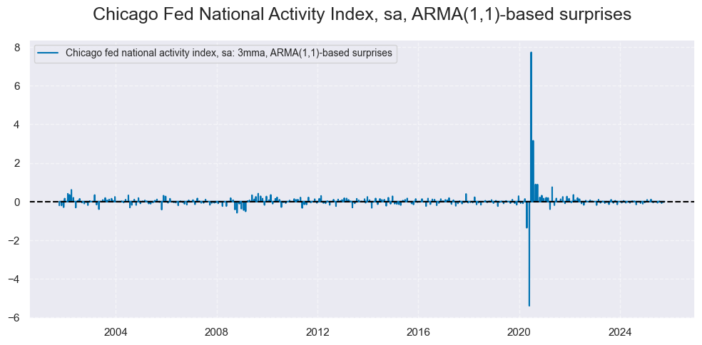
Label : Chicago Fed National Activity Index, sa, ARMA(1,1)-based surprises: 3mma / diff 3m/3m
Definition : Chicago Fed National Activity Index, seasonally adjusted, ARMA(1,1)-based surprises: 3 month moving average / difference of latest 3 months over previous 3 months
Notes :
-
Refer to the section on US Composite activity indicator for notes on the underlying data series.
-
Expected values for release dates are based on an “ARMA(1,1)” model. This is a simple univariate time series model that predicts increments based on an autoregressive component, i.e., last period’s value, and a moving average component, represented by last period’s error. The coefficients of the model are estimated sequentially based on the vintages of production indices. And each vintage-specific model produces a one-step-ahead forecast for the subsequent observation period.
Orders and inventories #
Ticker : DGORDERS_SA_P1M1ML1_ARMAS / DGORDERS_SA_P3M3ML3AR_ARMAS / DGORDERS_SA_P1M1ML12_ARMAS / DGORDERS_SA_P1M1ML12_3MMA_ARMAS
Label : Durable goods orders, sa, ARMA(1,1)-based surprises: %m/m / % 3m/3m AR / %oya / %oya, 3mma
Definition : New durable goods orders, ARMA(1,1)-based surprises: % month-on-month / % 3-month-moving average over prevous 3-month moving average annualized rate / % over a year ago / % over a year ago, 3-month moving average
Notes :
-
Refer to the section on US orders and inventories for notes on the underlying data series.
-
Expected values for release dates are based on an “ARMA(1,1)” model. This is a simple univariate time series model that predicts increments based on an autoregressive component, i.e., last period’s value, and a moving average component, represented by last period’s error. The coefficients of the model are estimated sequentially based on the vintages of production indices. And each vintage-specific model produces a one-step-ahead forecast for the subsequent observation period.
Ticker : DGORDERSXD_SA_P1M1ML1_ARMAS / DGORDERSXD_SA_P3M3ML3AR_ARMAS / DGORDERSXD_SA_P1M1ML12_ARMAS / DGORDERSXD_SA_P1M1ML12_3MMA_ARMAS
Label : Durable goods orders ex defense, sa, ARMA(1,1)-based surprises: %m/m / % 3m/3m AR / %oya / %oya, 3mma
Definition : New durable goods orders excluding defense, ARMA(1,1)-based surprises: % month-on-month / % 3-month-moving average over previous 3-month moving average annualized rate / % over a year ago / % over a year ago, 3-month moving average
Notes :
-
Refer to the section on US orders and inventories for notes on the underlying data series.
-
Expected values for release dates are based on an “ARMA(1,1)” model. This is a simple univariate time series model that predicts increments based on an autoregressive component, i.e., last period’s value, and a moving average component, represented by last period’s error. The coefficients of the model are estimated sequentially based on the vintages of production indices. And each vintage-specific model produces a one-step-ahead forecast for the subsequent observation period.
Ticker : BINVENTORIES_SA_P1M1ML1_ARMAS / BINVENTORIES_SA_P3M3ML3AR_ARMAS / BINVENTORIES_SA_P1M1ML12_ARMAS / BINVENTORIES_SA_P1M1ML12_3MMA_ARMAS
Label : Business inventories, sa, ARMA(1,1)-based surprises: %m/m / % 3m/3m AR / %oya / %oya, 3mma
Definition : Business inventories, seasonally adjusted, ARMA(1,1)-based surprises: % month-on-month / % 3-month-moving average over previous 3-month moving average annualized rate / % over a year ago / % over a year ago, 3-month moving average
Notes :
-
Refer to the section on US orders and inventories for notes on the underlying data series.
-
Expected values for release dates are based on an “ARMA(1,1)” model. This is a simple univariate time series model that predicts increments based on an autoregressive component, i.e., last period’s value, and a moving average component, represented by last period’s error. The coefficients of the model are estimated sequentially based on the vintages of production indices. And each vintage-specific model produces a one-step-ahead forecast for the subsequent observation period.
Private consumption #
Ticker : CONS_SA_P1M1ML12_ARMAS / CONS_SA_P1M1ML12_3MMA_ARMAS / CONS_SA_P3M3ML3AR_ARMAS
Label : Real consumption, sa, ARMA(1,1)-based surprises: %oya / %oya, 3mma / %3m/3m AR
Definition : Real personal consumption, seasonally adjusted, ARMA(1,1)-based surprises: % over a year ago / % over a year ago, 3-month moving average / % 3 months over previous 3 months annualized rate
Notes :
-
Refer to the section on US private consumption for notes on the underlying data series.
-
Expected values for release dates are based on an “ARMA(1,1)” model. This is a simple univariate time series model that predicts increments based on an autoregressive component, i.e., last period’s value, and a moving average component, represented by last period’s error. The coefficients of the model are estimated sequentially based on the vintages of production indices. And each vintage-specific model produces a one-step-ahead forecast for the subsequent observation period.
Ticker : RSALESXAF_SA_P1M1ML1_ARMAS / RSALESXAF_SA_P6M6ML6AR_ARMAS / RSALESXAF_SA_P1M1ML12_ARMAS / RSALESXAF_SA_P1M1ML12_3MMA_ARMAS
Label : Retail sales, ex autos and gas, ARMA(1,1)-based surprises: total, sa, %m/m / total, sa, %6m/6m AR / total, sa, %oya / total, sa, %oya, 3mma
Definition : Retail sales values, ex autos and gas, ARMA(1,1)-based surprises: total, sa, %m/m / total, sa, %6m/6m annualized rate / total, nsa, %oya / total, nsa, %oya 3mma
Notes :
-
Refer to the section on US private consumption for notes on the underlying data series.
-
Expected values for release dates are based on an “ARMA(1,1)” model. This is a simple univariate time series model that predicts increments based on an autoregressive component, i.e., last period’s value, and a moving average component, represented by last period’s error. The coefficients of the model are estimated sequentially based on the vintages of production indices. And each vintage-specific model produces a one-step-ahead forecast for the subsequent observation period.
Ticker : PERSINC_SA_P1M1ML12_ARMAS / PERSINC_SA_P1M1ML12_3MMA_ARMAS / PERSINC_SA_P3M3ML3AR_ARMAS
Label : Personal income, sa, ARMA(1,1)-based surprises, ARMA(1,1)-based surprises: %oya / %oya, 3mma / %3m/3m AR
Definition : Personal income, seasonally adjusted, ARMA(1,1)-based surprises, ARMA(1,1)-based surprises: % over a year ago / % over a year ago, 3-month moving average / % 3 months over previous 3 months annualized rate
Notes :
-
Refer to the section on US private consumption for notes on the underlying data series.
-
Expected values for release dates are based on an “ARMA(1,1)” model. This is a simple univariate time series model that predicts increments based on an autoregressive component, i.e., last period’s value, and a moving average component, represented by last period’s error. The coefficients of the model are estimated sequentially based on the vintages of production indices. And each vintage-specific model produces a one-step-ahead forecast for the subsequent observation period.
Ticker : CARSALES_SA_P1M1ML12_ARMAS / CARSALES_SA_P1M1ML12_3MMA_ARMAS
Label : Moto vehicle sales, sa, ARMA(1,1)-based surprises: %oya / %oya, 3mma
Definition : Moto vehicle sales, units, seasonally adjusted, ARMA(1,1)-based surprises: % over a year ago / % over a year ago, 3-month moving average
Notes :
-
Refer to the section on US private consumption for notes on the underlying data series.
-
Expected values for release dates are based on an “ARMA(1,1)” model. This is a simple univariate time series model that predicts increments based on an autoregressive component, i.e., last period’s value, and a moving average component, represented by last period’s error. The coefficients of the model are estimated sequentially based on the vintages of production indices. And each vintage-specific model produces a one-step-ahead forecast for the subsequent observation period.
Housing indicators #
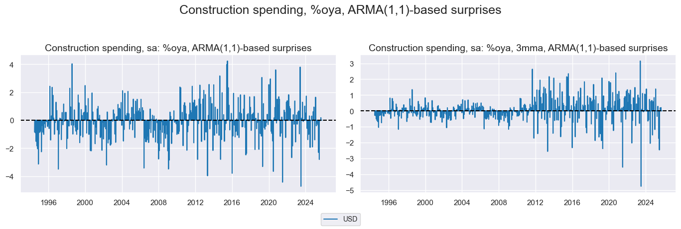
Ticker : CONSTRSPEND_SA_P1M1ML12_ARMAS / CONSTRSPEND_SA_P1M1ML12_3MMA_ARMAS
Label : Construction spending, sa, ARMA(1,1)-based surprises: %oya / %oya, 3mma
Definition : Construction spending in USD, seasonally adjusted, ARMA(1,1)-based surprises: % over a year ago / % over a year ago, 3-month moving average
Notes :
-
Refer to the section on US housing indicators for notes on the underlying data series.
-
Expected values for release dates are based on an “ARMA(1,1)” model. This is a simple univariate time series model that predicts increments based on an autoregressive component, i.e., last period’s value, and a moving average component, represented by last period’s error. The coefficients of the model are estimated sequentially based on the vintages of production indices. And each vintage-specific model produces a one-step-ahead forecast for the subsequent observation period.
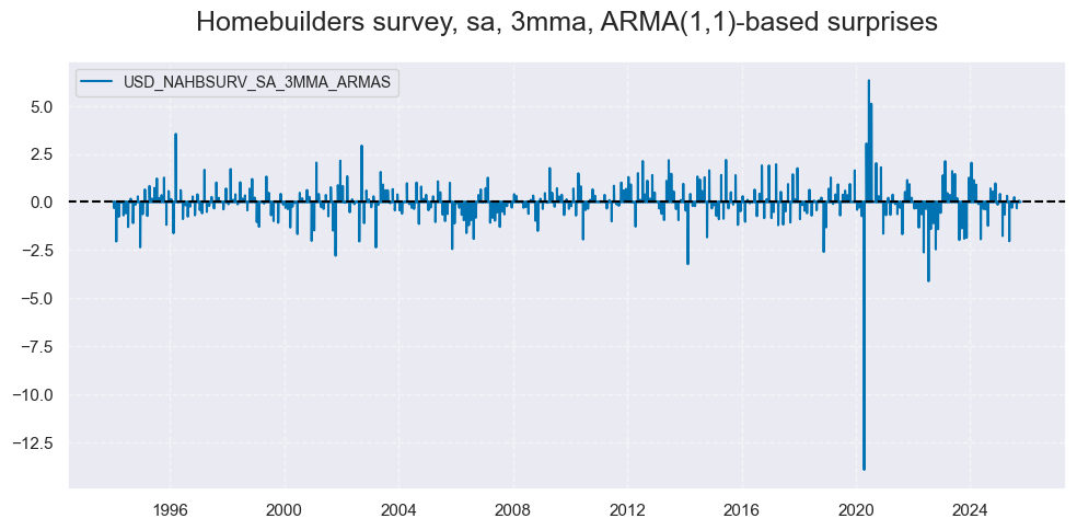
Ticker : NAHBSURV_SA_3MMA_ARMAS / NAHBSURV_SA_D3M3ML3_ARMAS
Label : Homebuilders survey, sa, ARMA(1,1)-based surprises: 3mma / diff 3m/3m
Definition : Housing market index of the homebuilders survey, seasonally adjuste, ARMA(1,1)-based surprises:: 3 month moving average / difference of latest 3 months over previous 3 months
Notes :
-
Refer to the section on US housing indicators for notes on the underlying data series.
-
Expected values for release dates are based on an “ARMA(1,1)” model. This is a simple univariate time series model that predicts increments based on an autoregressive component, i.e., last period’s value, and a moving average component, represented by last period’s error. The coefficients of the model are estimated sequentially based on the vintages of production indices. And each vintage-specific model produces a one-step-ahead forecast for the subsequent observation period.
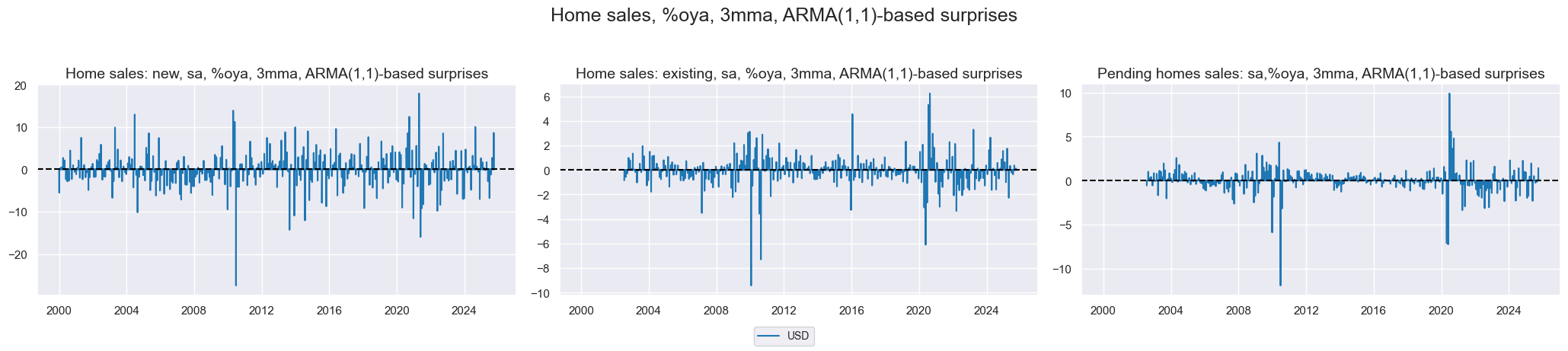
Ticker : NEWHOMESALES_SA_P1M1ML12_ARMAS / NEWHOMESALES_SA_P1M1ML12_3MMA_ARMAS / EXISTHOMESALES_SA_P1M1ML12_ARMAS / EXISTHOMESALES_SA_P1M1ML12_3MMA_ARMAS
Label : Home sales, ARMA(1,1)-based surprises: %oya, new / %oya, 3mma, new / %oya, existing / %oya, 3mma, existing
Definition : Home sales, ARMA(1,1)-based surprises: % over a year ago, new / % over a year ago, 3-month average, new / % over a year ago, existing / % over a year ago, 3-month average, existing
Notes :
-
Refer to the section on US housing indicators for notes on the underlying data series.
-
Expected values for release dates are based on an “ARMA(1,1)” model. This is a simple univariate time series model that predicts increments based on an autoregressive component, i.e., last period’s value, and a moving average component, represented by last period’s error. The coefficients of the model are estimated sequentially based on the vintages of production indices. And each vintage-specific model produces a one-step-ahead forecast for the subsequent observation period.
Ticker : PENDHOMESALES_SA_P1M1ML12_ARMAS / PENDHOMESALES_SA_P1M1ML12_3MMA_ARMAS
Label : Pending homes sales, ARMA(1,1)-based surprises: %oya / %oya, 3mma
Definition : Pending home sales, ARMA(1,1)-based surprises: percentage change over a year ago / percentage change over a year ago, 3-month average, change over the last three estimable months.
Notes :
-
Refer to the section on US housing indicators for notes on the underlying data series.
-
Expected values for release dates are based on an “ARMA(1,1)” model. This is a simple univariate time series model that predicts increments based on an autoregressive component, i.e., last period’s value, and a moving average component, represented by last period’s error. The coefficients of the model are estimated sequentially based on the vintages of production indices. And each vintage-specific model produces a one-step-ahead forecast for the subsequent observation period.
Labor market #
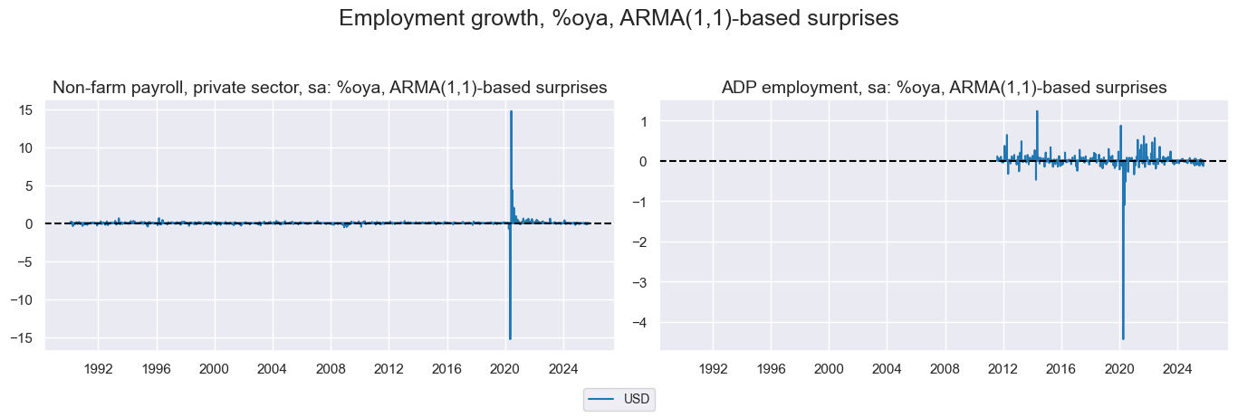
Ticker : NFPAYROLLPRIV_SA_P1M1ML1_ARMAS / NFPAYROLLPRIV_SA_P3M3ML3AR_ARMAS / NFPAYROLLPRIV_SA_P1M1ML12_ARMAS / NFPAYROLLPRIV_SA_P1M1ML12_3MMA_ARMAS
Label : Non-farm payroll, private sector, sa, ARMA(1,1)-based surprises: %m/m / %3m/3m / %oya / %oya, 3mma
Definition : Non-farm payroll, private sector, seasonally adjusted: % month-on-month / % 3-month moving average over previous 3-month moving average / % over a year ago / % over a year ago, 3-month moving average
Notes :
-
Refer to the section on US labor market for notes on the underlying data series.
-
Expected values for release dates are based on an “ARMA(1,1)” model. This is a simple univariate time series model that predicts increments based on an autoregressive component, i.e., last period’s value, and a moving average component, represented by last period’s error. The coefficients of the model are estimated sequentially based on the vintages of production indices. And each vintage-specific model produces a one-step-ahead forecast for the subsequent observation period.
Ticker : ADPEMPL_SA_P1M1ML1_ARMAS / ADPEMPL_SA_P3M3ML3AR_ARMAS / ADPEMPL_SA_P1M1ML12_ARMAS / ADPEMPL_SA_P1M1ML12_3MMA_ARMAS
Label : ADP employment, sa, ARMA(1,1)-based surprises: %m/m / %3m/3m / %oya / %oya, 3mma
Definition : ADP employment, seasonally adjusted, ARMA(1,1)-based surprises: % month-on-month / % 3-month moving average over previous 3-month moving average / % over a year ago / % over a year ago, 3-month moving average
Notes :
-
Refer to the section on US labor market for notes on the underlying data series.
-
Expected values for release dates are based on an “ARMA(1,1)” model. This is a simple univariate time series model that predicts increments based on an autoregressive component, i.e., last period’s value, and a moving average component, represented by last period’s error. The coefficients of the model are estimated sequentially based on the vintages of production indices. And each vintage-specific model produces a one-step-ahead forecast for the subsequent observation period.
Ticker : HOURLYWAGES_SA_P1M1ML1_ARMAS / HOURLYWAGES_SA_P3M3ML3AR_ARMAS / HOURLYWAGES_SA_P1M1ML12_ARMAS / HOURLYWAGES_SA_P1M1ML12_3MMA_ARMAS
Label : Hourly wages, sa, ARMA(1,1)-based surprises: %m/m / %3m/3m AR / %oya / %oya, 3mma
Definition : Average hourly wages, seasonally adjusted, ARMA(1,1)-based surprises: % month-on-month / % 3-month moving average over previous 3-month moving average annualized rate / % over a year ago / % over a year ago, 3-month moving average
Notes :
-
Refer to the section on US labor market for notes on the underlying data series.
-
Expected values for release dates are based on an “ARMA(1,1)” model. This is a simple univariate time series model that predicts increments based on an autoregressive component, i.e., last period’s value, and a moving average component, represented by last period’s error. The coefficients of the model are estimated sequentially based on the vintages of production indices. And each vintage-specific model produces a one-step-ahead forecast for the subsequent observation period.
Ticker : HOURLYCOMP_SA_P1Q1QL4_ARMAS
Label : Hourly compensation, sa, ARMA(1,1)-based surprises: % oya
Definition : Hourly compensation, seasonally adjusted, ARMA(1,1)-based surprises: % over a year ago
Notes : * Refer to the section on US labor market for notes on the underlying data series.
-
Expected values for release dates are based on an “ARMA(1,1)” model. This is a simple univariate time series model that predicts increments based on an autoregressive component, i.e., last period’s value, and a moving average component, represented by last period’s error. The coefficients of the model are estimated sequentially based on the vintages of production indices. And each vintage-specific model produces a one-step-ahead forecast for the subsequent observation period.
Ticker : HOURLYPROD_SA_P1Q1QL4_ARMAS
Label : Labor productivity, sa, ARMA(1,1)-based surprises: % oya
Definition : Labor productivity (output per hour), seasonally adjusted, ARMA(1,1)-based surprises: % over a year ago
Notes :
-
Refer to the section on US labor market for notes on the underlying data series.
-
Expected values for release dates are based on an “ARMA(1,1)” model. This is a simple univariate time series model that predicts increments based on an autoregressive component, i.e., last period’s value, and a moving average component, represented by last period’s error. The coefficients of the model are estimated sequentially based on the vintages of production indices. And each vintage-specific model produces a one-step-ahead forecast for the subsequent observation period.
Prices #
Ticker : IMPIH_NSA_P1M1ML12_ARMAS / IMPIH_NSA_P1M1ML12_3MMA_ARMAS
Label : Import price index, ARMA(1,1)-based surprises: %oya / %oya, 3mma
Definition : Import price index: % over a year ago / % over a year ago, 3-month moving average
Notes :
-
Refer to the section on US prices for notes on the underlying data series.
-
Expected values for release dates are based on an “ARMA(1,1)” model. This is a simple univariate time series model that predicts increments based on an autoregressive component, i.e., last period’s value, and a moving average component, represented by last period’s error. The coefficients of the model are estimated sequentially based on the vintages of production indices. And each vintage-specific model produces a one-step-ahead forecast for the subsequent observation period.
Ticker : IMPIC_NSA_P1M1ML12_ARMAS / IMPIC_NSA_P1M1ML12_3MMA_ARMAS
Label : Core import price index, ARMA(1,1)-based surprises: %oya / %oya, 3mma
Definition : Import price index excluding fuel: % over a year ago / % over a year ago, 3-month moving average
Notes :
-
Refer to the section on US prices for notes on the underlying data series.
-
Expected values for release dates are based on an “ARMA(1,1)” model. This is a simple univariate time series model that predicts increments based on an autoregressive component, i.e., last period’s value, and a moving average component, represented by last period’s error. The coefficients of the model are estimated sequentially based on the vintages of production indices. And each vintage-specific model produces a one-step-ahead forecast for the subsequent observation period.
Imports #
Only the standard Python data science packages and the specialized
macrosynergy
package are needed.
import os
import numpy as np
import pandas as pd
import matplotlib.pyplot as plt
import seaborn as sns
import math

import json
import yaml

import macrosynergy.management as msm
import macrosynergy.panel as msp
import macrosynergy.signal as mss
import macrosynergy.pnl as msn
import macrosynergy.visuals as msv


from macrosynergy.download import JPMaQSDownload

from timeit import default_timer as timer
from datetime import timedelta, date, datetime

import warnings

warnings.simplefilter("ignore")
The
JPMaQS
indicators we consider are downloaded using the J.P. Morgan Dataquery API interface within the
macrosynergy
package. This is done by specifying
ticker strings
, formed by appending an indicator category code
<category>
to a currency area code
<cross_section>
. These constitute the main part of a full quantamental indicator ticker, taking the form
DB(JPMAQS,<cross_section>_<category>,<info>)
, where
<info>
denotes the time series of information for the given cross-section and category. The following types of information are available:
-
valuegiving the latest available values for the indicator -
eop_lagreferring to days elapsed since the end of the observation period -
mop_lagreferring to the number of days elapsed since the mean observation period -
gradedenoting a grade of the observation, giving a metric of real time information quality.
After instantiating the
JPMaQSDownload
class within the
macrosynergy.download
module, one can use the
download(tickers,start_date,metrics)
method to easily download the necessary data, where
tickers
is an array of ticker strings,
start_date
is the first collection date to be considered and
metrics
is an array comprising the times series information to be downloaded.
cids = ["USD"]
main = [
    "NYMANU_SA_3MMA_ARMAS",
    "NYMANU_SA_D3M3ML3_ARMAS",
    "PHILMANU_SA_3MMA_ARMAS",
    "PHILMANU_SA_D3M3ML3_ARMAS",
    "CBCCONF_SA_3MMA_ARMAS",
    "CBCCONF_SA_D3M3ML3_ARMAS",
    "NAHBSURV_SA_3MMA_ARMAS",
    "NAHBSURV_SA_D3M3ML3_ARMAS",
    "ISMMANU_SA_3MMA_ARMAS",
    "ISMMANU_SA_D3M3ML3_ARMAS",
    "ISMSERV_SA_3MMA_ARMAS",
    "ISMSERV_SA_D3M3ML3_ARMAS",
    "UMCCONF_NSA_3MMA_ARMAS",
    "UMCCONF_NSA_D3M3ML3_ARMAS",
    "CONSTRSPEND_SA_P1M1ML12_3MMA_ARMAS",
    "CONSTRSPEND_SA_P1M1ML12_ARMAS",
    "EXISTHOMESALES_SA_P1M1ML12_3MMA_ARMAS",
    "EXISTHOMESALES_SA_P1M1ML12_ARMAS",
    "NEWHOMESALES_SA_P1M1ML12_3MMA_ARMAS",
    "NEWHOMESALES_SA_P1M1ML12_ARMAS",
    "PENDHOMESALES_SA_P1M1ML12_3MMA_ARMAS",
    "PENDHOMESALES_SA_P1M1ML12_ARMAS",
    "BINVENTORIES_SA_P1M1ML12_ARMAS",
    "BINVENTORIES_SA_P1M1ML1_ARMAS",
    "BINVENTORIES_SA_P3M3ML3AR_ARMAS",
    "BINVENTORIES_SA_P1M1ML12_3MMA_ARMAS",
    "DGORDERS_SA_P1M1ML12_ARMAS",
    "DGORDERS_SA_P1M1ML1_ARMAS",
    "DGORDERS_SA_P3M3ML3AR_ARMAS",
    "DGORDERS_SA_P1M1ML12_3MMA_ARMAS",
    "DGORDERSXD_SA_P1M1ML12_ARMAS",
    "DGORDERSXD_SA_P1M1ML1_ARMAS",
    "DGORDERSXD_SA_P3M3ML3AR_ARMAS",
    "DGORDERSXD_SA_P1M1ML12_3MMA_ARMAS",
    "NFPAYROLLPRIV_SA_P1M1ML12_ARMAS",
    "NFPAYROLLPRIV_SA_P1M1ML1_ARMAS",
    "NFPAYROLLPRIV_SA_P3M3ML3AR_ARMAS",
    "NFPAYROLLPRIV_SA_P1M1ML12_3MMA_ARMAS",
    "HOURLYWAGES_SA_P1M1ML12_ARMAS",
    "HOURLYWAGES_SA_P1M1ML1_ARMAS",
    "HOURLYWAGES_SA_P3M3ML3AR_ARMAS",
    "HOURLYWAGES_SA_P1M1ML12_3MMA_ARMAS",
    "ADPEMPL_SA_P1M1ML12_ARMAS",
    "ADPEMPL_SA_P1M1ML1_ARMAS",
    "ADPEMPL_SA_P3M3ML3AR_ARMAS",
    "ADPEMPL_SA_P1M1ML12_3MMA_ARMAS",
    "IMPIH_NSA_P1M1ML12_ARMAS",
    "IMPIH_NSA_P1M1ML12_3MMA_ARMAS",
    "IMPIC_NSA_P1M1ML12_ARMAS",
    "IMPIC_NSA_P1M1ML12_3MMA_ARMAS",
    "RSALESXAF_SA_P1M1ML1_ARMAS",
    "RSALESXAF_SA_P6M6ML6AR_ARMAS",
    "RSALESXAF_SA_P1M1ML12_3MMA_ARMAS",
    "RSALESXAF_SA_P1M1ML12_ARMAS",
    "CONS_SA_P1M1ML12_ARMAS",
    "CONS_SA_P3M3ML3AR_ARMAS",
    "CONS_SA_P1M1ML12_3MMA_ARMAS",
    "PERSINC_SA_P1M1ML12_ARMAS",
    "PERSINC_SA_P3M3ML3AR_ARMAS",
    "PERSINC_SA_P1M1ML12_3MMA_ARMAS",
    "HOURLYPROD_SA_P1Q1QL4_ARMAS",
    "HOURLYCOMP_SA_P1Q1QL4_ARMAS",
    "CARSALES_SA_P1M1ML12_3MMA_ARMAS",
    "CARSALES_SA_P1M1ML12_ARMAS",
    "CFNAI_SA_3MMA_ARMAS",
    "CFNAI_SA_D3M3ML3_ARMAS"
]

econ = [
    "GBF02YXR_NSA",
    "GBF05YXR_NSA",
    "GBF10YXR_NSA",
    "EQXR_NSA",
    "EQNASDAQXR_NSA",
    "EQRUSSELLXR_NSA",
    "DU05YXR_NSA",
    "DU02YXR_NSA",
    "DU10YXR_NSA"

]
xcats = main
# Download series from J.P. Morgan DataQuery by tickers

start_date = "1990-01-01"
tickers = [cid + "_" + xcat for cid in cids for xcat in (xcats+econ)]
print(f"Maximum number of tickers is {len(tickers)}")

# Retrieve credentials

client_id: str = os.getenv("DQ_CLIENT_ID")
client_secret: str = os.getenv("DQ_CLIENT_SECRET")

# Download from DataQuery

with JPMaQSDownload(client_id=client_id, client_secret=client_secret) as downloader:
    start = timer()
    assert downloader.check_connection()
    df = downloader.download(
        tickers=tickers,
        start_date=start_date,
        show_progress=True,
        metrics=["value", "eop_lag", "mop_lag", "grading"],
        suppress_warning=True,
    )
    end = timer()

dfd = df.copy()

print("Download time from DQ: " + str(timedelta(seconds=end - start)))
Maximum number of tickers is 75
Downloading data from JPMaQS.
Timestamp UTC:  2025-10-08 08:56:00
Connection successful!
Requesting data: 100%|█████████████████████████████████████████████████████████████████| 15/15 [00:03<00:00,  4.67it/s]
Downloading data: 100%|████████████████████████████████████████████████████████████████| 15/15 [00:26<00:00,  1.75s/it]
Download time from DQ: 0:00:33.319448
# Assign categories to high level labels to make subsequent analysis more readable

cat_dict = {
    "Business": ["NYMANU", "PHILMANU", "ISMSERV", "ISMMANU","CFNAI"],
    "Orders": ["BINVENTORIES", "DGORDERS", "DGORDERSXD"],
    "Consumption": [
        "CBCCONF",
        "UMCCONF",
        "CARSALES",
        "CONS",
        "PERSINC",
        "RSALESXAF",
    ],
    "Housing": [
        "NAHBSURV",
        "EXISTHOMESALES",
        "NEWHOMESALES",
        "PENDHOMESALES",
        "CONSTRSPEND",
    ],
    "Labor": [
        "ADPEMPL",
        "NFPAYROLLPRIV",
        "HOURLYWAGES",
        "HOURLYCOMP",
        "HOURLYPROD",
    ],
    "Prices": [ "IMPIC", "IMPIH"],
}
order = ["Business", "Orders", "Consumption", "Housing", "Labor", "Prices"]


def cat_dict_to_column(cat_string, cat_dict):
    for cat_list in cat_dict:
        if cat_string in cat_dict[cat_list]:
            cat_keys = [*cat_dict.keys()]

            return cat_keys.index(cat_list)
        else:
            continue


def cat_dict_to_key(cat_string, cat_dict):
    for cat_list in cat_dict:
        if cat_string in cat_dict[cat_list]:
            return cat_list
        else:
            continue
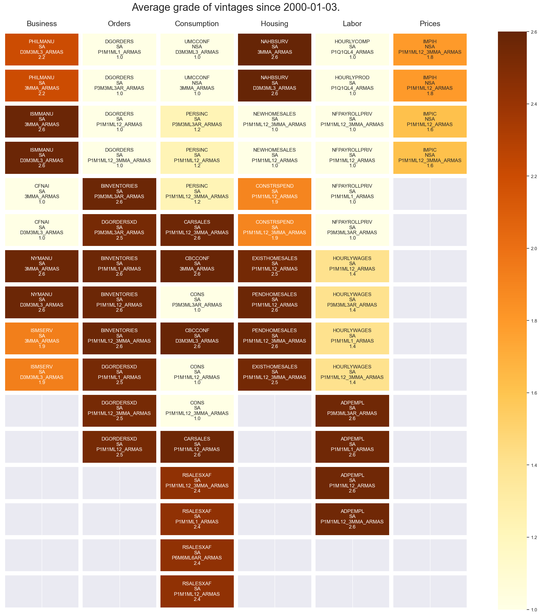
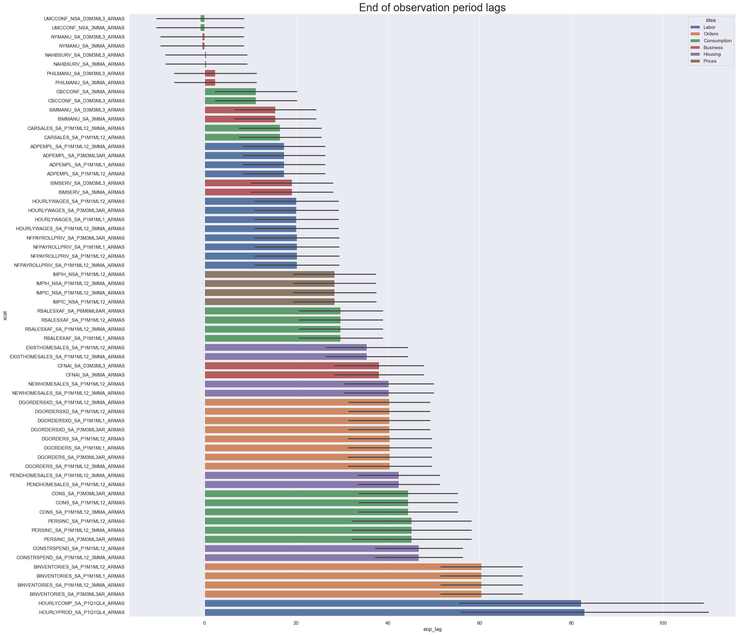
Availability #
66
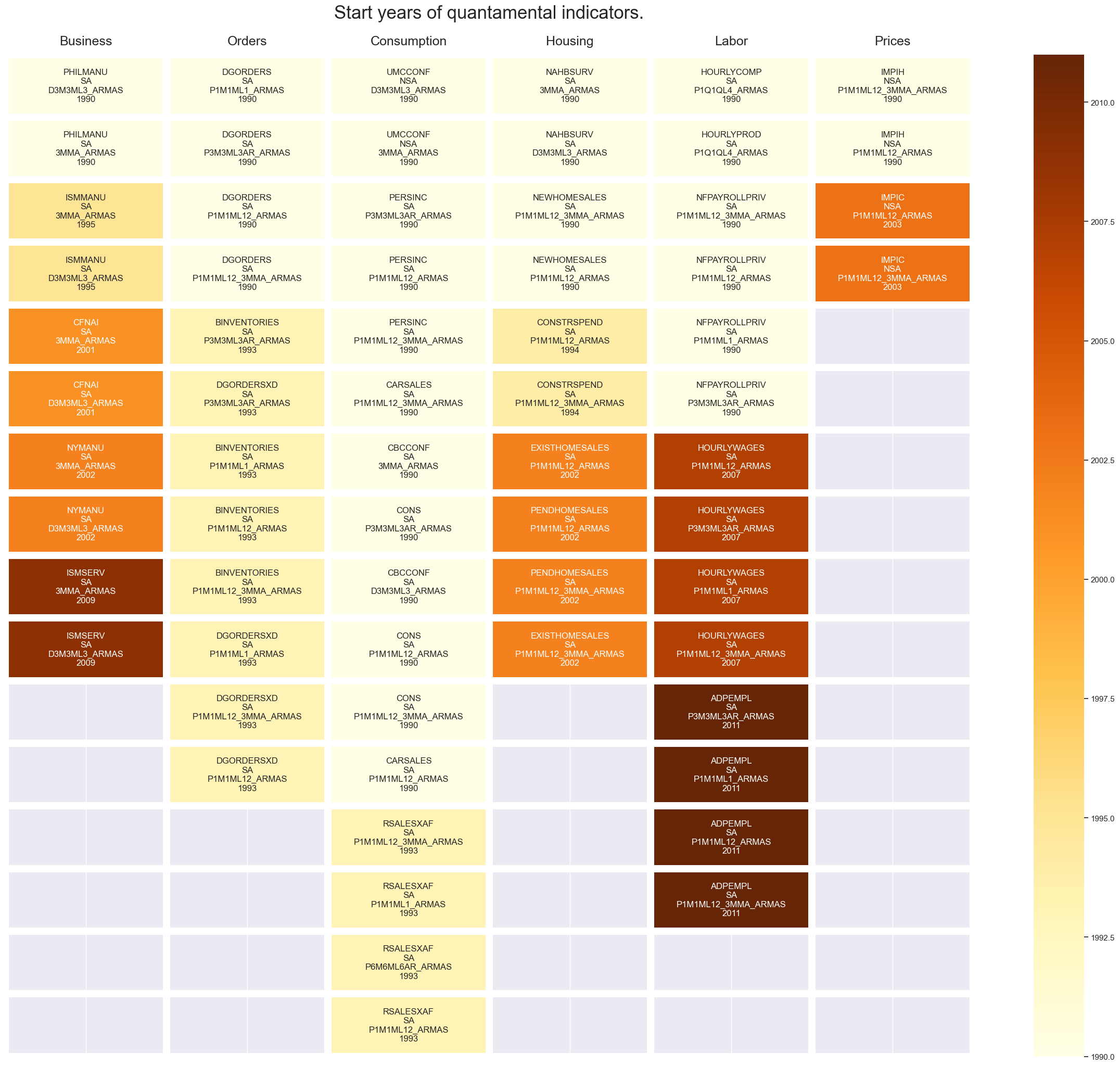
Last updated: 2025-10-08
History #
# Create definition dictionary for ease in subsequent analysis

def_dict = {
    'ISMMANU_SA_3MMA_ARMAS': 'ISM manufacturing survey, sa: 3mma, ARMA(1,1)-based surprises',
    'ISMMANU_SA_D3M3ML3_ARMAS': 'ISM manufacturing survey, sa: diff 3m/3m, ARMA(1,1)-based surprises',
    'ISMSERV_SA_3MMA_ARMAS': 'ISM services survey, sa: 3mma, ARMA(1,1)-based surprises',
    'ISMSERV_SA_D3M3ML3_ARMAS': 'ISM services survey, sa:diff 3m/3m, ARMA(1,1)-based surprises',
    'PHILMANU_SA_3MMA_ARMAS': 'Philadelphia manufacturing survey, sa: 3mma, ARMA(1,1)-based surprises',
    'PHILMANU_SA_D3M3ML3_ARMAS': 'Philadelphia manufacturing survey, sa: diff 3m/3m, ARMA(1,1)-based surprises',
    'NYMANU_SA_3MMA_ARMAS': 'Empire State manufacturing survey, sa: 3mma, ARMA(1,1)-based surprises',
    'NYMANU_SA_D3M3ML3_ARMAS': 'Empire State manufacturing survey, sa: diff 3m/3m, ARMA(1,1)-based surprises',
    'DGORDERS_SA_P1M1ML1_ARMAS': 'Durable goods orders, sa: %m/m, ARMA(1,1)-based surprises',
    'DGORDERS_SA_P3M3ML3AR_ARMAS': 'Durable goods orders, sa: %3m/3m, ARMA(1,1)-based surprises',
    'DGORDERS_SA_P1M1ML12_ARMAS': 'Durable goods orders, sa: %oya, ARMA(1,1)-based surprises',
    'DGORDERS_SA_P1M1ML12_3MMA_ARMAS': 'Durable goods orders, sa: %oya, 3mma, ARMA(1,1)-based surprises',
    'DGORDERSXD_SA_P1M1ML1_ARMAS': 'Durable goods orders ex defense, sa: %m/m, ARMA(1,1)-based surprises',
    'DGORDERSXD_SA_P3M3ML3AR_ARMAS': 'Durable goods orders ex defense, sa:  %3m/3m, ARMA(1,1)-based surprises',
    'DGORDERSXD_SA_P1M1ML12_ARMAS': 'Durable goods orders ex defense, sa:  %oya, ARMA(1,1)-based surprises',
    'DGORDERSXD_SA_P1M1ML12_3MMA_ARMAS': 'Durable goods orders ex defense, sa: %oya, 3mma, ARMA(1,1)-based surprises',
    'BINVENTORIES_SA_P1M1ML1_ARMAS': 'Business inventories, sa: %m/m, ARMA(1,1)-based surprises',
    'BINVENTORIES_SA_P3M3ML3AR_ARMAS': 'Business inventories, sa: %3m/3m, ARMA(1,1)-based surprises',
    'BINVENTORIES_SA_P1M1ML12_ARMAS': 'Business inventories, sa: %oya, ARMA(1,1)-based surprises',
    'BINVENTORIES_SA_P1M1ML12_3MMA_ARMAS': 'Business inventories, sa: %oya, 3mma, ARMA(1,1)-based surprises',
    'CFNAI_SA_3MMA_ARMAS': 'Chicago fed national activity index, sa: 3mma, ARMA(1,1)-based surprises',
    'CFNAI_SA_D3M3ML3_ARMAS': 'Chicago fed national activity index, sa: diff 3m/3m, ARMA(1,1)-based surprises',
    'CBCCONF_SA_3MMA_ARMAS': 'Conference board consumer confidence, sa: 3mma, ARMA(1,1)-based surprises',
    'CBCCONF_SA_D3M3ML3_ARMAS': 'Conference board consumer confidence, sa: diff 3m/3m, ARMA(1,1)-based surprises',
    'UMCCONF_NSA_3MMA_ARMAS': 'University of Michigan consumer sentiment, nsa: 3mma, ARMA(1,1)-based surprises',
    'UMCCONF_NSA_D3M3ML3_ARMAS': 'University of Michigan consumer sentiment, nsa: diff 3m/3m, ARMA(1,1)-based surprises',
    'CONS_SA_P1M1ML12_ARMAS': 'Real consumption, sa: %oya, ARMA(1,1)-based surprises',
    'CONS_SA_P1M1ML12_3MMA_ARMAS': 'Real consumption, sa: %oya, 3mma , ARMA(1,1)-based surprises',
    'CONS_SA_P3M3ML3AR_ARMAS': 'Real consumption, sa: %3m/3m, ARMA(1,1)-based surprises',
    'RSALES_SA_P1M1ML1_ARMAS': 'Retail sales: total, sa, %m/m, ARMA(1,1)-based surprises',
    'RSALES_SA_P6M6ML6AR_ARMAS': 'Retail sales: total, sa, %6m/6m, ARMA(1,1)-based surprises',
    'RSALES_SA_P1M1ML12_ARMAS': 'Retail sales: total, sa, %oya, ARMA(1,1)-based surprises',
    'RSALES_SA_P1M1ML12_3MMA_ARMAS': 'Retail sales: total, sa ,%oya, 3mma, ARMA(1,1)-based surprises',
    'RSALESXAF_SA_P1M1ML1_ARMAS': 'Retail sales: ex autos and gas, sa, ARMA(1,1)-based surprises',
    'RSALESXAF_SA_P6M6ML6AR_ARMAS': 'Retail sales: ex autos and gas, sa, %6m/6m, ARMA(1,1)-based surprises',
    'RSALESXAF_SA_P1M1ML12_ARMAS': 'Retail sales: ex autos and gas, sa, %oya, ARMA(1,1)-based surprises',
    'RSALESXAF_SA_P1M1ML12_3MMA_ARMAS': 'Retail sales: ex autos and gas, sa, %oya, 3mma, ARMA(1,1)-based surprises',
    'PERSINC_SA_P1M1ML12_ARMAS': 'Personal income, sa: %oya, ARMA(1,1)-based surprises',
    'PERSINC_SA_P1M1ML12_3MMA_ARMAS': 'Personal income, sa: %oya, 3mma, ARMA(1,1)-based surprises',
    'PERSINC_SA_P3M3ML3AR_ARMAS': 'Personal income, sa: %3m/3m, ARMA(1,1)-based surprises',
    'CARSALES_SA_P1M1ML12_ARMAS': 'Moto vehicle sales, sa: %oya, ARMA(1,1)-based surprises',
    'CARSALES_SA_P1M1ML12_3MMA_ARMAS': 'Moto vehicle sales, sa: %oya, 3mma, ARMA(1,1)-based surprises',
    'CONSTRSPEND_SA_P1M1ML12_ARMAS': 'Construction spending, sa: %oya, ARMA(1,1)-based surprises',
    'CONSTRSPEND_SA_P1M1ML12_3MMA_ARMAS': 'Construction spending, sa: %oya, 3mma, ARMA(1,1)-based surprises',
    'NAHBSURV_SA_3MMA_ARMAS': 'Homebuilders survey, sa: 3mma, ARMA(1,1)-based surprises',
    'NAHBSURV_SA_D3M3ML3_ARMAS': 'Homebuilders survey, sa: diff 3m/3m, ARMA(1,1)-based surprises',
    'NEWHOMESALES_SA_P1M1ML12_ARMAS': 'Home sales: new, sa, %oya, ARMA(1,1)-based surprises',
    'NEWHOMESALES_SA_P1M1ML12_3MMA_ARMAS': 'Home sales: new, sa, %oya, 3mma, ARMA(1,1)-based surprises',
    'EXISTHOMESALES_SA_P1M1ML12_ARMAS': 'Home sales: existing, sa, %oya, ARMA(1,1)-based surprises',
    'EXISTHOMESALES_SA_P1M1ML12_3MMA_ARMAS': 'Home sales: existing, sa, %oya, 3mma, ARMA(1,1)-based surprises',
    'PENDHOMESALES_SA_P1M1ML12_ARMAS': 'Pending homes sales: sa, %oya, ARMA(1,1)-based surprises',
    'PENDHOMESALES_SA_P1M1ML12_3MMA_ARMAS': 'Pending homes sales: sa,%oya, 3mma, ARMA(1,1)-based surprises',
    'INJLCLAIMS_SA_D4W4WL4_ARMAS': 'Initial jobless claims, sa: dif 4w/4w, ARMA(1,1)-based surprises',
    'INJLCLAIMS_SA_D4W4WL52_ARMAS': 'Initial jobless claims, sa: dif oya, 4wma, ARMA(1,1)-based surprises',
    'INJLCLAIMS_SA_4WMAv5YMM_ARMAS': 'Initial jobless claims, sa: %4wma vs 5yma, ARMA(1,1)-based surprises',
    'INJLCLAIMS_SA_4WMAv10YMM_ARMAS': 'Initial jobless claims, sa: %4wma vs 10yma, ARMA(1,1)-based surprises',
    'COJLCLAIMS_SA_D4W4WL4_ARMAS': 'Continuing jobless claims, sa: dif 4w/4w, ARMA(1,1)-based surprises',
    'COJLCLAIMS_SA_D4W4WL52_ARMAS': 'Continuing jobless claims, sa: dif oya, 4wma, ARMA(1,1)-based surprises',
    'COJLCLAIMS_SA_4WMAv5YMM_ARMAS': 'Continuing jobless claims, sa: %4wma vs 5yma, ARMA(1,1)-based surprises',
    'COJLCLAIMS_SA_4WMAv10YMM_ARMAS': 'Continuing jobless claims, sa: %4wma vs 10yma, ARMA(1,1)-based surprises',
    'NFPAYROLLPRIV_SA_P1M1ML1_ARMAS': 'Non-farm payroll, private sector, sa: %m/m, ARMA(1,1)-based surprises',
    'NFPAYROLLPRIV_SA_P3M3ML3_ARMAS': 'Non-farm payroll, private sector, sa: %3m/3m, ARMA(1,1)-based surprises',
    'NFPAYROLLPRIV_SA_P1M1ML12_ARMAS': 'Non-farm payroll, private sector, sa: %oya, ARMA(1,1)-based surprises',
    'NFPAYROLLPRIV_SA_P1M1ML12_3MMA_ARMAS': 'Non-farm payroll, private sector, sa: %oya, 3mma, ARMA(1,1)-based surprises',
    'ADPEMPL_SA_P1M1ML1_ARMAS': 'ADP employment, sa: %m/m, ARMA(1,1)-based surprises',
    'ADPEMPL_SA_P3M3ML3AR_ARMAS': 'ADP employment, sa: %3m/3m, ARMA(1,1)-based surprises',
    'ADPEMPL_SA_P1M1ML12_ARMAS': 'ADP employment, sa: %oya, ARMA(1,1)-based surprises',
    'ADPEMPL_SA_P1M1ML12_3MMA_ARMAS': 'ADP employment, sa: %oya, 3mma, ARMA(1,1)-based surprises',
    'HOURLYWAGES_SA_P1M1ML1_ARMAS': 'Hourly wages, sa: %m/m, ARMA(1,1)-based surprises',
    'HOURLYWAGES_SA_P3M3ML3AR_ARMAS': 'Hourly wages, sa: %3m/3m, ARMA(1,1)-based surprises',
    'HOURLYWAGES_SA_P1M1ML12_ARMAS': 'Hourly wages, sa: %oya, ARMA(1,1)-based surprises',
    'HOURLYWAGES_SA_P1M1ML12_3MMA_ARMAS': 'Hourly wages, sa: %oya, 3mma, ARMA(1,1)-based surprises',
    'HOURLYCOMP_SA_P1Q1QL4_ARMAS': 'Hourly compensation, sa: % oya, ARMA(1,1)-based surprises',
    'HOURLYPROD_SA_P1Q1QL4_ARMAS': 'Labor productivity, sa: % oya, ARMA(1,1)-based surprises',
    'CPIUH_SA_P1M1ML1_ARMAS': 'Consumer price index, sa: %m/m, ARMA(1,1)-based surprises',
    'CPIUH_SA_P6M6ML6AR_ARMAS': 'Consumer price index, sa: %6m/6m, ARMA(1,1)-based surprises',
    'CPIUH_NSA_P1M1ML12_ARMAS': 'Consumer price index, nsa: %oya, ARMA(1,1)-based surprises',
    'CPIUH_NSA_P1M1ML12_3MMA_ARMAS': 'Consumer price index, nsa: %oya, 3mma, ARMA(1,1)-based surprises',
    'CPIUC_SA_P1M1ML1_ARMAS': 'Core CPI, sa: %m/m, ARMA(1,1)-based surprises',
    'CPIUC_SA_P6M6ML6AR_ARMAS': 'Core CPI, sa: %6m/6m, ARMA(1,1)-based surprises',
    'CPIUC_NSA_P1M1ML12_ARMAS': 'Core CPI, nsa: %oya, ARMA(1,1)-based surprises',
    'CPIUC_NSA_P1M1ML12_3MMA_ARMAS': 'Core CPI, nsa: %oya, 3mma, ARMA(1,1)-based surprises',
    'PPIH_SA_P1M1ML1_ARMAS': 'Producer price index, sa: %m/m, ARMA(1,1)-based surprises',
    'PPIH_SA_P6M6ML6AR_ARMAS': 'Producer price index, sa: %6m/6m, ARMA(1,1)-based surprises',
    'PPIH_NSA_P1M1ML12_ARMAS': 'Producer price index, nsa: %oya, ARMA(1,1)-based surprises',
    'PPIH_NSA_P1M1ML12_3MMA_ARMAS': 'Producer price index, nsa: %oya, 3mma, ARMA(1,1)-based surprises',
    'PPIC_SA_P1M1ML1_ARMAS': 'Core PPI, sa: %m/m, ARMA(1,1)-based surprises',
    'PPIC_SA_P6M6ML6AR_ARMAS': 'Core PPI, sa: %6m/6m, ARMA(1,1)-based surprises',
    'PPIC_NSA_P1M1ML12_ARMAS': 'Core PPI, nsa: %oya, ARMA(1,1)-based surprises',
    'PPIC_NSA_P1M1ML12_3MMA_ARMAS': 'Core PPI, nsa: %oya, 3mma, ARMA(1,1)-based surprises',
    'IMPIH_NSA_P1M1ML12_ARMAS': 'Import price index, nsa: %oya, ARMA(1,1)-based surprises',
    'IMPIH_NSA_P1M1ML12_3MMA_ARMAS': 'Import price index, nsa: %oya, 3mma, ARMA(1,1)-based surprises',
    'IMPIC_NSA_P1M1ML12_ARMAS': 'Core import price index, nsa: %oya, ARMA(1,1)-based surprises',
    'IMPIC_NSA_P1M1ML12_3MMA_ARMAS': 'Core import price index, nsa: %oya, 3mma, ARMA(1,1)-based surprises'
}
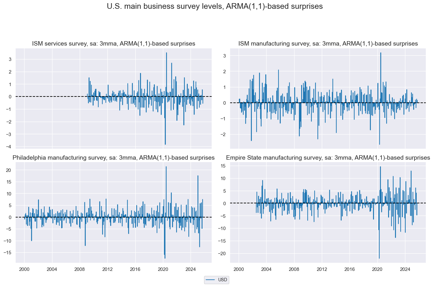
Business surveys #
Surprises among the various business surveys have have differing magnitudes but all spike around Covid.
xcatx = ["ISMSERV", "ISMMANU", "PHILMANU", "NYMANU"]
xcatxx = [xc + "_SA_3MMA_ARMAS" for xc in xcatx]
labels = [def_dict[key] for key in xcatxx]
msp.view_timelines(
    dfd,
    xcats=xcatxx,
    cids=["USD"],
    title="U.S. main business survey levels, ARMA(1,1)-based surprises",
    xcat_labels=labels,
    start="2000-01-01",
    title_adj=1.05,
    ncol=2,
    legend_fontsize=10,
    size=(10, 5),
    same_y=False,
    xcat_grid=True
)
Composite activity indicator #
xcatxx = ["CFNAI_SA_3MMA_ARMAS"]
labels = [def_dict[key] for key in xcatxx]
msp.view_timelines(
    dfd,
    xcats=xcatxx,
    cids=["USD"],
    title="Chicago Fed National Activity Index, sa, ARMA(1,1)-based surprises",
    xcat_labels=labels,
    title_adj=1.05,
    legend_fontsize=10,
    start="2001-01-01",
    size=(10, 5),
)
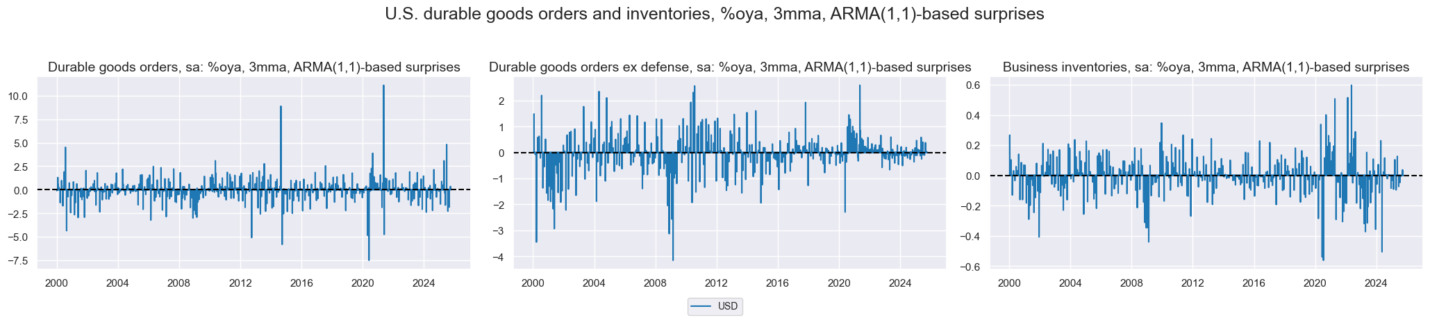
Orders and inventories #
Durable goods including defense are much more prone to surprises compared to durable goods excluding defense.
xcatx = ["DGORDERS", "DGORDERSXD", "BINVENTORIES"]
xcatxx = [xc + "_SA_P1M1ML12_3MMA_ARMAS" for xc in xcatx]
labels = [def_dict[key] for key in xcatxx]
msp.view_timelines(
    dfd,
    xcats=xcatxx,
    cids=["USD"],
    title="U.S. durable goods orders and inventories, %oya, 3mma, ARMA(1,1)-based surprises",
    xcat_labels=labels,
    title_adj=1.05,
    legend_fontsize=10,
    start="2000-01-01",
    size=(10, 5),
    same_y=False,
    xcat_grid=True
)
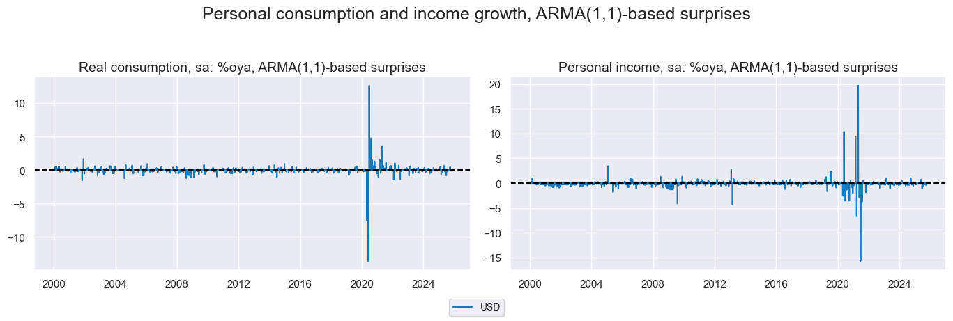
Private consumption #
Income and spending #
Unlike many other indicators personal income did not have a major negative surprise around Covid but instead directly afterwards.
xcatxx = ["CONS_SA_P1M1ML12_ARMAS", "PERSINC_SA_P1M1ML12_ARMAS"]
labels = [def_dict[key] for key in xcatxx]
msp.view_timelines(
    dfd,
    xcats=xcatxx,
    cids=["USD"],
    title="Personal consumption and income growth, ARMA(1,1)-based surprises",
    xcat_labels=labels,
    title_adj=1.05,
    legend_fontsize=10,
    start="2000-01-01",
    size=(10, 5),
    same_y=False,
    xcat_grid=True
)
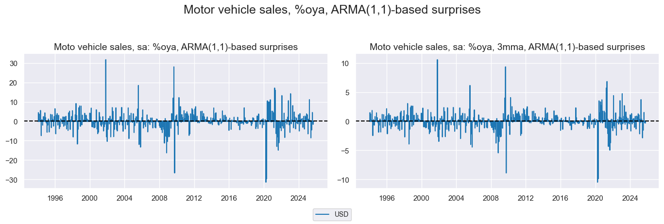
xcatxx = ["CARSALES_SA_P1M1ML12_ARMAS", "CARSALES_SA_P1M1ML12_3MMA_ARMAS"]
labels = [def_dict[key] for key in xcatxx]
msp.view_timelines(
    dfd,
    xcats=xcatxx,
    cids=["USD"],
    title="Motor vehicle sales, %oya, ARMA(1,1)-based surprises",
    title_adj=1.05,
    legend_fontsize=10,
    xcat_labels=labels,
    start="1994-01-01",
    size=(10, 5),
    same_y=False,
    xcat_grid=True
)
Housing indicators #
While construction spending has no outliers home sales had outliers around the financial crash and Covid.
xcatxx = ["CONSTRSPEND_SA_P1M1ML12_ARMAS", "CONSTRSPEND_SA_P1M1ML12_3MMA_ARMAS"]
labels = [def_dict[key] for key in xcatxx]
msp.view_timelines(
    dfd,
    xcats=xcatxx,
    cids=["USD"],
    title="Construction spending, %oya, ARMA(1,1)-based surprises",
    title_adj=1.05,
    legend_fontsize=10,
    xcat_labels=labels,
    start="1994-01-01",
    size=(10, 5),
        same_y=False,
    xcat_grid=True
)
xcatxx = ["NAHBSURV_SA_3MMA_ARMAS"]
msp.view_timelines(
    dfd,
    xcats=xcatxx,
    cids=["USD"],
    title="Homebuilders survey, sa, 3mma, ARMA(1,1)-based surprises",
    title_adj=1.05,
    legend_fontsize=10,
    start="1994-01-01",
    size=(10, 5),
)
xcatx = ["NEWHOMESALES", "EXISTHOMESALES", "PENDHOMESALES"]
xcatxx = [xc + "_SA_P1M1ML12_3MMA_ARMAS" for xc in xcatx]
labels = [def_dict[key] for key in xcatxx]
msp.view_timelines(
    dfd,
    xcats=xcatxx,
    cids=["USD"],
    title="Home sales, %oya, 3mma, ARMA(1,1)-based surprises",
    legend_fontsize=10,
    title_adj=1.05,
    xcat_labels=labels,
    start="2000-01-01",
    size=(10, 5),
            same_y=False,
    xcat_grid=True
)
Labor market #
Labor market had such large surprises around Covid it dwarfs the rest of the surprises.
Employment growth #
xcatx = ["NFPAYROLLPRIV", "ADPEMPL"]
xcatxx = [xc + "_SA_P1M1ML12_ARMAS" for xc in xcatx]
labels = [def_dict[key] for key in xcatxx]
msp.view_timelines(
    dfd,
    xcats=xcatxx,
    cids=["USD"],
    title="Employment growth, %oya, ARMA(1,1)-based surprises",
    xcat_labels=labels,
    legend_fontsize=10,
    title_adj=1.05,
    start="1990-01-01",
    size=(10, 5),
    same_y= False,
    xcat_grid=True
)
Prices #
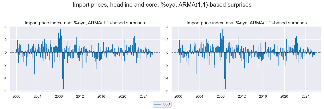
Import prices seem to have a larger surprise around the 2008 financial crash instead of Covid compared to other indicators
xcatxx = ["IMPIH_NSA_P1M1ML12_ARMAS", "IMPIH_NSA_P1M1ML12_ARMAS"]
labels = [def_dict[key] for key in xcatxx]
msp.view_timelines(
    dfd,
    xcats=xcatxx,
    cids=["USD"],
    title="Import prices, headline and core, %oya, ARMA(1,1)-based surprises",
    xcat_labels=labels,
    title_adj=1.05,
    legend_fontsize=10,
    start="2000-01-01",
    size=(10, 5),
    same_y= False,
    xcat_grid=True
)
Importance #
Relevant research #
“Financial markets are expected to respond to such news, especially when the actual numbers released are not in line with the expected values.” Gu, Chen and Chen, Denghui and Stan, Raluca, Investor Sentiment and the Market Reaction to Macroeconomic News
Empirical clues #
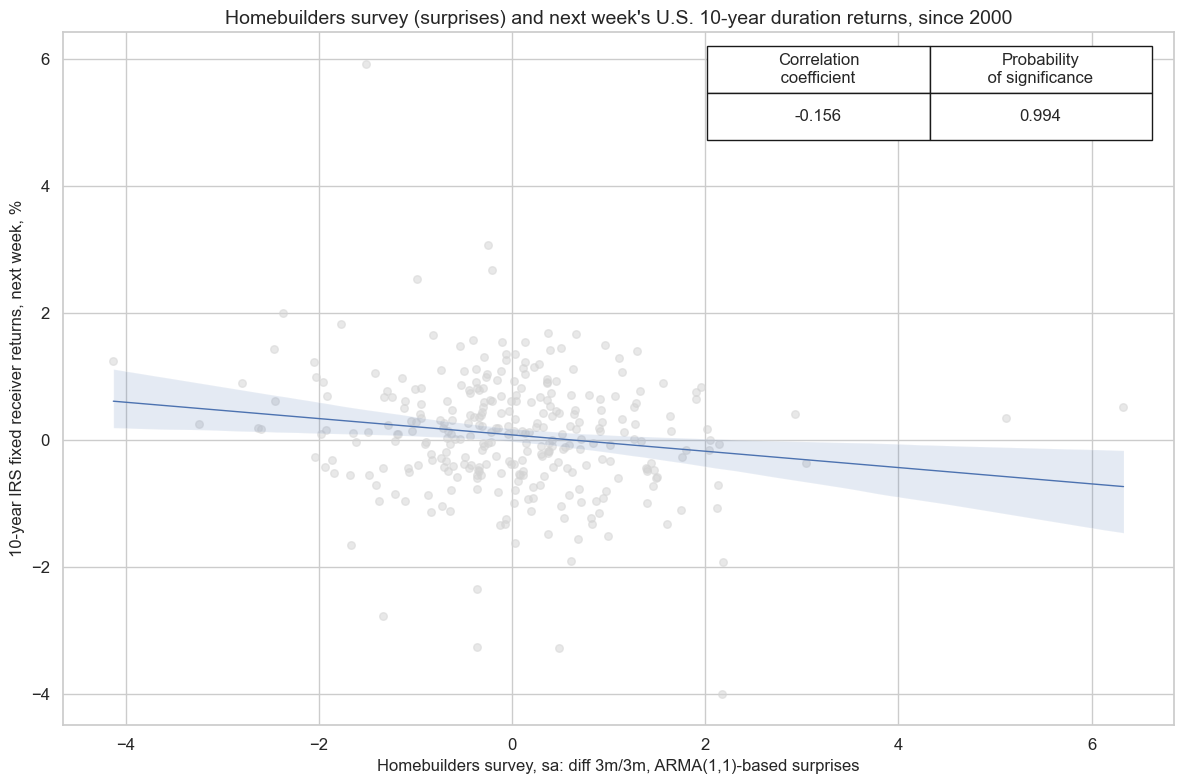
Surprises to short-term dynamics of the homebuilders survey have displayed negative and highly significant predictive power with respect to subsequent weekly duration returns, i.e., returns. Strength in the survey means that builders feel optimistic about housing market conditions. Bright prospects for housing increase expected demand for mortgages and reduce the need for monetary policy support. Both justify higher long-term yields.
cidx = ["USD"]

cr = msp.CategoryRelations(
    dfd,
    xcats=["NAHBSURV_SA_3MMA_ARMAS", "DU10YXR_NSA"],
    cids=cidx,
    freq="W",
    lag=1,
    xcat_aggs=["sum", "sum"],
    fwin=1,
    start="2000-01-01",
    xcat_trims=[10, None]
)

cr.reg_scatter(
    labels=False,
    coef_box="upper right",
    prob_est="map",
    title = "Homebuilders survey (surprises) and next week's U.S. 10-year duration returns, since 2000",
    xlab="Homebuilders survey, sa: diff 3m/3m, ARMA(1,1)-based surprises",
    ylab="10-year IRS fixed receiver returns, next week, %",
    remove_zero_predictor=True,
)
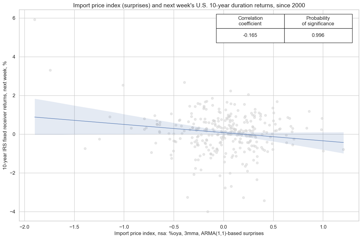
Surprises to import price growth also predicted next week duration returns negatively with high significance. Higher imported inflation may also lift local inflation forecasts, forcing the central bank to be more vigilant.
cidx = ["USD"]

cr = msp.CategoryRelations(
    dfd,
    xcats=["IMPIH_NSA_P1M1ML12_3MMA_ARMAS", "DU10YXR_NSA"],
    cids=cidx,
    freq="W",
    lag=1,
    xcat_aggs=["sum", "sum"],
    fwin=1,
    start="2000-01-01",
    # xcat_trims=[10, None]
)

cr.reg_scatter(
    labels=False,
    coef_box="upper right",
    prob_est="map",
    title = "Import price index (surprises) and next week's U.S. 10-year duration returns, since 2000",
    xlab="Import price index, nsa: %oya, 3mma, ARMA(1,1)-based surprises",
    ylab="10-year IRS fixed receiver returns, next week, %",
    remove_zero_predictor=True,
)
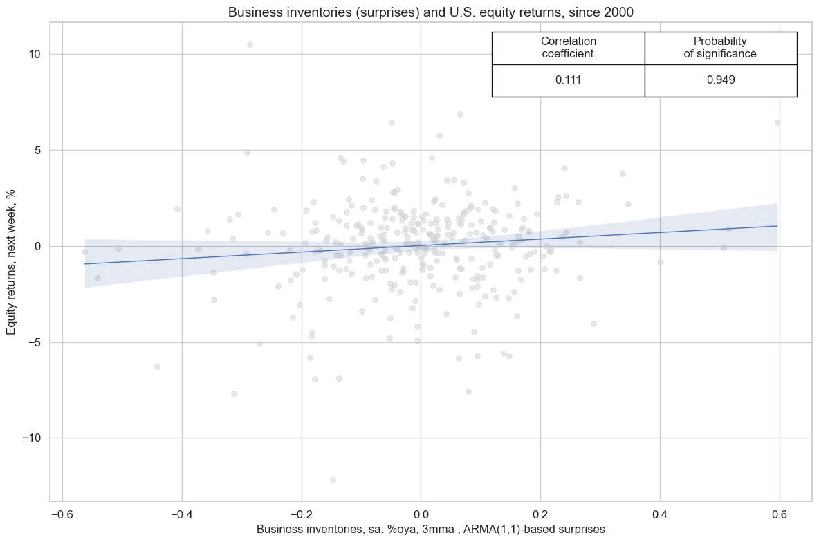
Surprises to business inventory growth trends have positively predicted subsequent weekly equity index future returns. This may possibly reflect the pro-cyclical nature of inventory growth, which often reflects stronger expected sales.
cidx = ["USD"]

cr = msp.CategoryRelations(
    dfd,
    xcats=["BINVENTORIES_SA_P1M1ML12_3MMA_ARMAS", "EQXR_NSA"],
    cids=cidx,
    freq="W",
    lag=1,
    xcat_aggs=["sum", "sum"],
    fwin=1,
    start="2000-01-01",
    # xcat_trims=[1, None]
)

cr.reg_scatter(
    labels=False,
    coef_box="upper right",
    prob_est="map",
    title = "Business inventories (surprises) and U.S. equity returns, since 2000",
    xlab="Business inventories, sa: %oya, 3mma , ARMA(1,1)-based surprises",
    ylab="Equity returns, next week, %",
    remove_zero_predictor=True,
)
Appendices #
Appendix 1: Quantamental economic surprises #
Quantamental economic surprises are defined as deviations of point-in-time quantamental indicators from expected values. Expected values are estimated predictions of an informed market participant. Following this definition there are two types of surprises that jointly make up economic surprise indicators:
• A first print event is the difference between a quantamental indicator on a release date and its expected value. A release date is the day on which any underlying economic time series adds an observation period. Expected values are estimated, typically based on econometric models and information prior to the release date. A quantamental data surprise is always specific to the prediction model or statistical learning process.
• A pure revision event is the change in a quantamental indicator on a non-release date. It arises from revisions of data for previously released observation periods. Per default, it is assumed that all revisions are surprises, i.e., that the latest reported value for an observation period is the best predictor its value after revisions. Note that any revisions published on a release date become part of the first print event.
A quantamental indicator of economic surprises records the values of these two events on the dates they become known. It records zero values for all other dates. Models for predicting indicator values always use the latest vintage of the underlying data series. They are typically applied to increments, i.e., differences or log differences of volume, value or price indices. The predicted next increment produces an expected new vintage, and the expected new vintage implies a new derived expected quantamental indicator, such as an annual growth rate or moving average. Note than in this way predictions automatically account for “base effects”, i.e., predictable changes in growth rates that arise from unusually sharp increase of declines in index levels of the base period, for example a year ago.