Macro-enhanced trend following for bond markets #
Get packages and JPMaQS data #
# >>> Define constants <<< #
import os

# Minimum Macrosynergy package version required for this notebook
MIN_REQUIRED_VERSION: str = "0.1.32"

# DataQuery credentials: Remember to replace with your own client ID and secret
DQ_CLIENT_ID: str = os.getenv("DQ_CLIENT_ID")
DQ_CLIENT_SECRET: str = os.getenv("DQ_CLIENT_SECRET")

# Define any Proxy settings required (http/https)
PROXY = {}

# Start date for the data (argument passed to the JPMaQSDownloader class)
START_DATE: str = "1992-01-01"
# ! pip install macrosynergy --upgrade
# Standard library imports
from typing import List, Tuple, Dict
import warnings
import os
import itertools

import numpy as np
import pandas as pd
from pandas import Timestamp
import matplotlib.pyplot as plt
import matplotlib as mpl
import seaborn as sns
from scipy.stats import chi2

# Macrosynergy package imports
import macrosynergy.management as msm
import macrosynergy.panel as msp
import macrosynergy.pnl as msn
import macrosynergy.visuals as msv
import macrosynergy.signal as mss
from macrosynergy.management.utils import merge_categories
from macrosynergy.visuals import ScoreVisualisers

from macrosynergy.download import JPMaQSDownload

warnings.simplefilter("ignore")
# Cross sections
cids_gb = ["USD"]

# Countries used for panel calculations
cids_add = ["EUR", "JPY", "GBP", "USD", "AUD", "CAD", "CHF", "NOK", "NZD", "SEK"]  # additional countries for scoring
cids_ecos = cids_gb + cids_add  # all areas used for economic analysis
cids = cids_ecos + ["DEM"]  # add Germany as representative issuer in euro area
# Category tickers
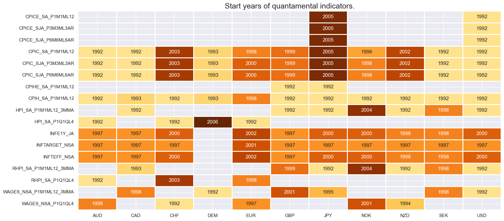
infl = [
"CPIH_SA_P1M1ML12",
"CPIHE_SA_P1M1ML12",
"CPIC_SA_P1M1ML12",
"CPICE_SA_P1M1ML12",
"CPIC_SJA_P3M3ML3AR",
"CPICE_SJA_P3M3ML3AR",
"CPIC_SJA_P6M6ML6AR",
"CPICE_SJA_P6M6ML6AR",
"INFE1Y_JA",
"INFTEFF_NSA",
"INFTARGET_NSA",
"WAGES_NSA_P1Q1QL4",
"WAGES_NSA_P1M1ML12_3MMA",
]
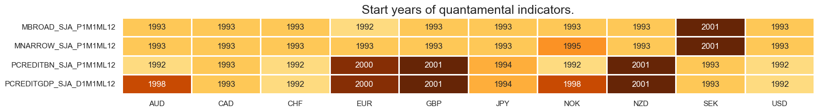
moncred = [
"MNARROW_SJA_P1M1ML12",
"MBROAD_SJA_P1M1ML12",
"PCREDITBN_SJA_P1M1ML12",
"PCREDITGDP_SJA_D1M1ML12"
]
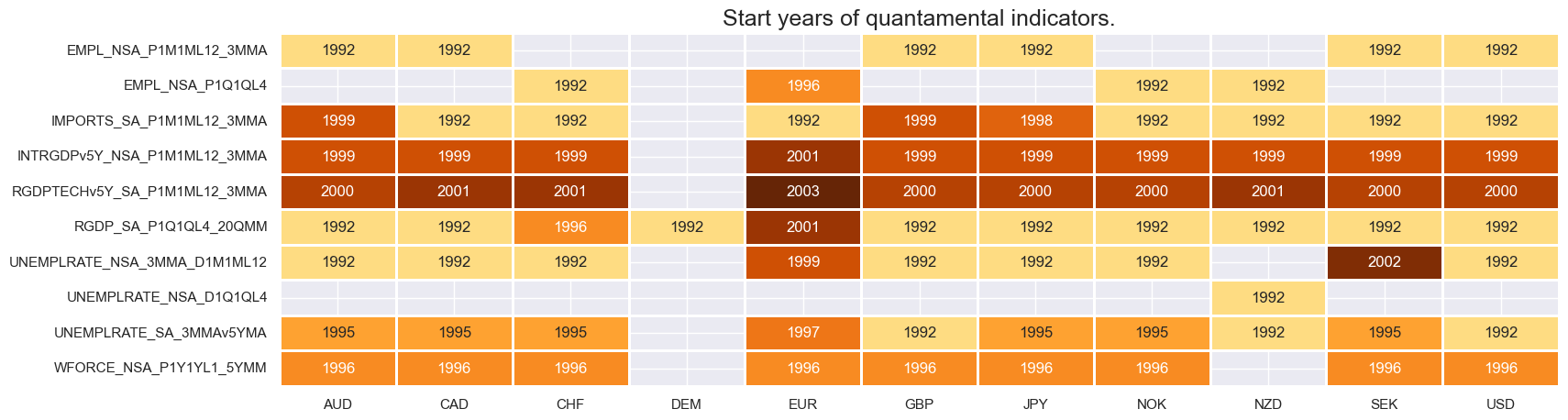
growth = [
"INTRGDPv5Y_NSA_P1M1ML12_3MMA",
"RGDPTECHv5Y_SA_P1M1ML12_3MMA",
"RGDP_SA_P1Q1QL4_20QMM",
"IMPORTS_SA_P1M1ML12_3MMA",
]
labour = [
"UNEMPLRATE_NSA_3MMA_D1M1ML12",
"UNEMPLRATE_NSA_D1Q1QL4",
"EMPL_NSA_P1M1ML12_3MMA",
"EMPL_NSA_P1Q1QL4",
"UNEMPLRATE_SA_3MMAv5YMA",
"WFORCE_NSA_P1Y1YL1_5YMM",
]
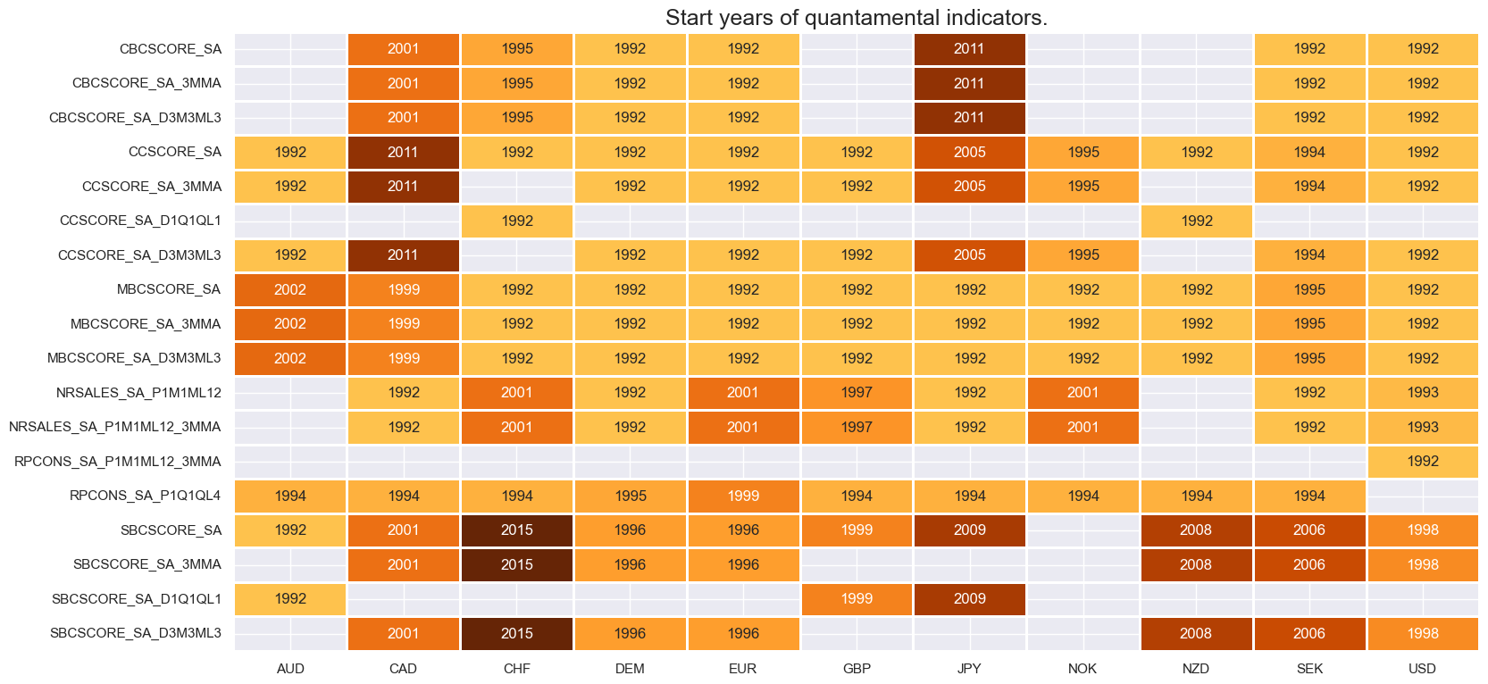
confidence = [
"RPCONS_SA_P1Q1QL4",
"RPCONS_SA_P1M1ML12_3MMA",
"MBCSCORE_SA",
"SBCSCORE_SA",
"CBCSCORE_SA",
"CCSCORE_SA",
"MBCSCORE_SA_3MMA",
"SBCSCORE_SA_3MMA",
"CCSCORE_SA_3MMA",
"CBCSCORE_SA_3MMA",
"CCSCORE_SA_D1Q1QL1",
"CCSCORE_SA_D3M3ML3",
"SBCSCORE_SA_D1Q1QL1",
"SBCSCORE_SA_D3M3ML3",
"CBCSCORE_SA_D1Q1QL1",
"CBCSCORE_SA_D3M3ML3",
"MBCSCORE_SA_D1Q1QL1",
"MBCSCORE_SA_D3M3ML3",
"NRSALES_SA_P1M1ML12",
"NRSALES_SA_P1M1ML12_3MMA",
]
hpinf = [
"HPI_SA_P1M1ML12_3MMA",
"RHPI_SA_P1M1ML12_3MMA",
"HPI_SA_P1Q1QL4",
"RHPI_SA_P1Q1QL4",
]
main = infl + confidence + moncred + growth + labour + hpinf
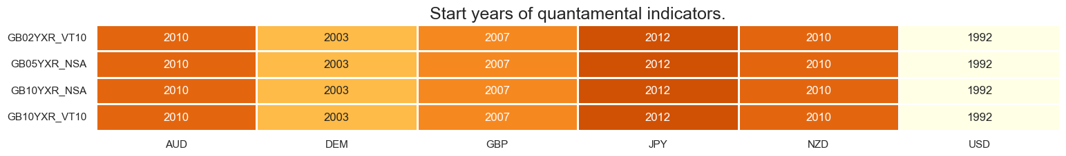
rets = [
"GB05YXR_NSA",
"GB10YXR_NSA",
"GB02YXR_VT10",
"GB10YXR_VT10",
]
xcats = main + rets
tickers = [cid + "_" + xcat for cid in cids for xcat in xcats]
print(f"Maximum number of tickers is {len(tickers)}")

# Download series from J.P. Morgan DataQuery by tickers

client_id: str = os.getenv("DQ_CLIENT_ID")
client_secret: str = os.getenv("DQ_CLIENT_SECRET")

with JPMaQSDownload(client_id=client_id, client_secret=client_secret) as dq:
    df = dq.download(
        tickers=tickers,
        start_date="1992-01-01",
        suppress_warning=True,
        metrics=[
            "value",
        ],
        show_progress=True,
    )
Maximum number of tickers is 660
Downloading data from JPMaQS.
Timestamp UTC:  2024-12-06 14:00:05
Connection successful!
Requesting data: 100%|██████████| 31/31 [00:07<00:00,  4.02it/s]
Downloading data: 100%|██████████| 31/31 [00:42<00:00,  1.38s/it]
Some expressions are missing from the downloaded data. Check logger output for complete list.
206 out of 605 expressions are missing. To download the catalogue of all available expressions and filter the unavailable expressions, set `get_catalogue=True` in the call to `JPMaQSDownload.download()`.
Some dates are missing from the downloaded data.
2 out of 8595 dates are missing.
scols = ["cid", "xcat", "real_date", "value"]  # required columns
dfx = df[scols].copy()
dfx.info()
<class 'pandas.core.frame.DataFrame'>
RangeIndex: 2918774 entries, 0 to 2918773
Data columns (total 4 columns):
 #   Column     Dtype
---  ------     -----
 0   cid        object
 1   xcat       object
 2   real_date  datetime64[ns]
 3   value      float64
dtypes: datetime64[ns](1), float64(1), object(2)
memory usage: 89.1+ MB
Availability and renamings #
Downloaded category groups #
xcatx = moncred
msm.check_availability(df, xcats=xcatx, cids=cids, missing_recent=False)
xcatx = infl + hpinf
msm.check_availability(df, xcats=xcatx, cids=cids, missing_recent=False)
xcatx = growth + labour
msm.check_availability(df, xcats=xcatx, cids=cids, missing_recent=False)
xcatx = confidence
msm.check_availability(df, xcats=xcatx, cids=cids, missing_recent=False)
xcatx = rets
msm.check_availability(df, xcats=xcatx, cids=cids, missing_recent=False)
Renamings #
# Rename quarterly categories to equivalent monthly tickers

dict_repl = {
    "RPCONS_SA_P1Q1QL4": "RPCONS_SA_P1M1ML12_3MMA",
    "EMPL_NSA_P1Q1QL4" : "EMPL_NSA_P1M1ML12_3MMA",
    "UNEMPLRATE_NSA_D1Q1QL4" : "UNEMPLRATE_NSA_3MMA_D1M1ML12",
    "WAGES_NSA_P1Q1QL4" : "WAGES_NSA_P1M1ML12_3MMA",
    "HPI_SA_P1Q1QL4": "HPI_SA_P1M1ML12_3MMA",
    "RHPI_SA_P1Q1QL4": "RHPI_SA_P1M1ML12_3MMA",
    "CCSCORE_SA_D1Q1QL1": "CCSCORE_SA_D3M3ML3",
    "SBCSCORE_SA_D1Q1QL1": "SBCSCORE_SA_D3M3ML3",
    "CBCSCORE_SA_D1Q1QL1": "CBCSCORE_SA_D3M3ML3",
    "MBCSCORE_SA_D1Q1QL1": "MBCSCORE_SA_D3M3ML3",
}

for key, value in dict_repl.items():
    dfx["xcat"] = dfx["xcat"].str.replace(key, value)

# Rename surveys of countries with quarterly data as equivalent monthly ones

cidx = list(set(cids_ecos) - set(dfx.loc[dfx['xcat'] == "SBCSCORE_SA_3MMA", :]['cid'].unique()))
dict_repl = {
"SBCSCORE_SA": "SBCSCORE_SA_3MMA"
}
for key, value in dict_repl.items():
    dfx.loc[dfx['cid'].isin(cidx), 'xcat'] = dfx.loc[dfx['cid'].isin(cidx), 'xcat'].str.replace(key, value)

cidx = list(set(cids_ecos) - set(dfx.loc[dfx['xcat'] == "CCSCORE_SA_3MMA", :]['cid'].unique()))
dict_repl = {
 "CCSCORE_SA": "CCSCORE_SA_3MMA"
}
for key, value in dict_repl.items():
    dfx.loc[dfx['cid'].isin(cidx), 'xcat'] = dfx.loc[dfx['cid'].isin(cidx), 'xcat'].str.replace(key, value)
# Stitching early and regular short-term core inflation

dict_merge = {
    "CPICC_SJA_P3M3ML3AR": ["CPICE_SJA_P3M3ML3AR", "CPIC_SJA_P3M3ML3AR"],
    "CPICC_SJA_P6M6ML6AR": ["CPICE_SJA_P6M6ML6AR", "CPIC_SJA_P6M6ML6AR"],
    "CPICC_SA_P1M1ML12": ["CPICE_SA_P1M1ML12", "CPIC_SA_P1M1ML12"],
    "CPIHC_SA_P1M1ML12": ["CPIHE_SA_P1M1ML12", "CPIH_SA_P1M1ML12"],
}
for key, value in dict_merge.items():
    dfa = merge_categories(dfx, value , key, cids_ecos)
    dfx = msm.update_df(dfx, dfa).reset_index(drop=True)
# # Define German bunds as euro area targets

# filt = dfx['xcat'].isin(rets) & (dfx['cid'] == "DEM")
# dfx.loc[filt, 'cid'] = dfx.loc[filt, "cid"].str.replace("DEM", "EUR")
xcatx = rets
cidx = cids_gb
msm.check_availability(dfx, xcats=xcatx, cids=cidx, missing_recent=False)

# Backward-extension of INFTARGET_NSA

# Duplicate targets
cidx = cids_ecos
calcs = [f"INFTARGET_BX = INFTARGET_NSA"]
dfa = msp.panel_calculator(dfx, calcs, cids=cidx)

# Add all dates back to 1990 to the frame, filling "value " with NaN
all_dates = np.sort(dfx['real_date'].unique())
all_combinations = pd.DataFrame(
    list(itertools.product(dfa['cid'].unique(), dfa['xcat'].unique(), all_dates)),
    columns=['cid', 'xcat', 'real_date']
)
dfax = pd.merge(all_combinations, dfa, on=['cid', 'xcat', 'real_date'], how='left')

# Backfill the values with first target value
dfax = dfax.sort_values(by=['cid', 'xcat', 'real_date'])
dfax['value'] = dfax.groupby(['cid', 'xcat'])['value'].bfill()

dfx = msm.update_df(dfx, dfax)

# Extended effective inflation target by hierarchical merging

hierarchy = ["INFTEFF_NSA", "INFTARGET_BX"]
dfa = merge_categories(dfx, xcats=hierarchy, new_xcat="INFTEFF_BX")
dfx = msm.update_df(dfx, dfa)
Transformations and checks #
Benchmarks #
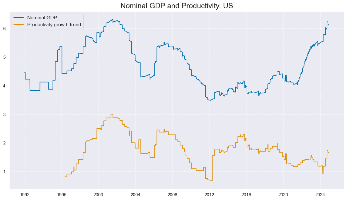
# Preparatory calculations
calcs = [
    "NGDP = RGDP_SA_P1Q1QL4_20QMM + INFTEFF_BX", # Expected nominal GDP growth
    "PROD = RGDP_SA_P1Q1QL4_20QMM - WFORCE_NSA_P1Y1YL1_5YMM", # Productivity growth trend
]
dfa = msp.panel_calculator(dfx, calcs=calcs, cids=cids)
dfx = msm.update_df(dfx, dfa)

xnomgrowth = list(dfa['xcat'].unique())
cidx = cids_gb
xcatx = ['NGDP', 'PROD']
# xnomgrowth

msp.view_timelines(
    dfx,
    xcats=xcatx,
    cids=cidx,
    ncol=2,
    title='Nominal GDP and Productivity, US',
    start="1992-01-01",
    same_y=False,
    xcat_labels=['Nominal GDP', 'Productivity growth trend']
)
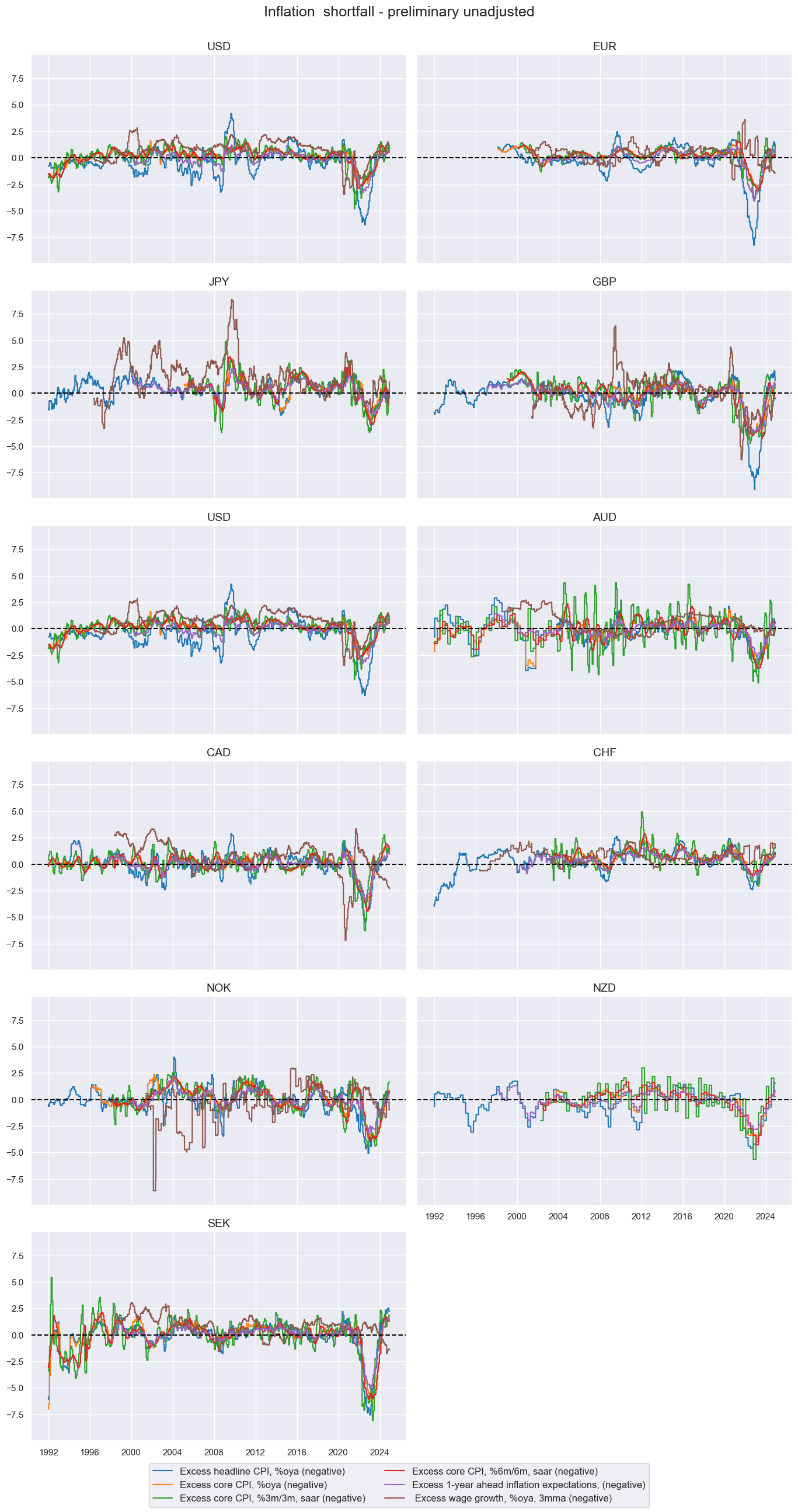
Inflation shortfall #
# Transformations

cidx = cids_ecos
calcs = []

infs = ["CPICC_SJA_P3M3ML3AR", "CPICC_SA_P1M1ML12", "CPIHC_SA_P1M1ML12", "CPICC_SJA_P6M6ML6AR", "INFE1Y_JA"]
wages = ["WAGES_NSA_P1M1ML12_3MMA"]

for xc in wages:
    calcs += [f"X{xc} = ( {xc} - PROD - INFTEFF_BX )" ]

for xc in infs:
    calcs += [f"X{xc} = ( {xc} - INFTEFF_BX )"]

dfa = msp.panel_calculator(dfx, calcs=calcs, cids=cidx)
dfx = msm.update_df(dfx, dfa)
# Collect categories, labels, and presumed impact signs

cidx = cids_ecos
dict_base = {
    "XCPIHC_SA_P1M1ML12": "Excess headline CPI, %oya (negative)",
    "XCPICC_SA_P1M1ML12": "Excess core CPI, %oya (negative)",
    "XCPICC_SJA_P3M3ML3AR": "Excess core CPI, %3m/3m, saar (negative)",
    "XCPICC_SJA_P6M6ML6AR": "Excess core CPI, %6m/6m, saar (negative)",
    "XINFE1Y_JA": "Excess 1-year ahead inflation expectations, (negative)",
    "XWAGES_NSA_P1M1ML12_3MMA": " Excess wage growth, %oya, 3mma (negative)",
}

# Set correct signs for all categories and created amended dictionary

negs = [key for key, value in dict_base.items() if value.endswith("(negative)")]

calcs = []
for xc in negs:
    calcs += [f"{xc}_NEG = - {xc}"]
dfa = msp.panel_calculator(dfx, calcs=calcs, cids=cidx)
dfx = msm.update_df(dfx, dfa)

keys_sa = [
    key + "_NEG" if value.strip().endswith("(negative)") else key
    for key, value in dict_base.items()
]

dict_xinf = dict(zip(keys_sa, dict_base.values()))  # dict with correct keys and labels
cidx = cids_ecos
xcatx = list(dict_xinf.keys())

msp.view_timelines(
    dfx,
    xcats=xcatx,
    cids=cidx,
    ncol=2,
    start="1992-01-01",
    same_y=True,
    title='Inflation  shortfall - preliminary unadjusted',
    xcat_labels=list(dict_xinf.values())
)
# Calculate standardized and winsorized values based on all countries

cidx = cids_ecos
xcatx = list(dict_xinf.keys())
dfa = pd.DataFrame(columns=list(dfx.columns))

for xc in xcatx:
    dfaa = msp.make_zn_scores(
        dfx,
        xcat=xc,
        cids=cidx,
        sequential=True,
        min_obs=261 * 5,
        neutral="zero",
        pan_weight=1,
        thresh=3,
        postfix="_ZN",
        est_freq="m",
    )
    dfa = msm.update_df(dfa, dfaa)

dfx = msm.update_df(dfx, dfa)
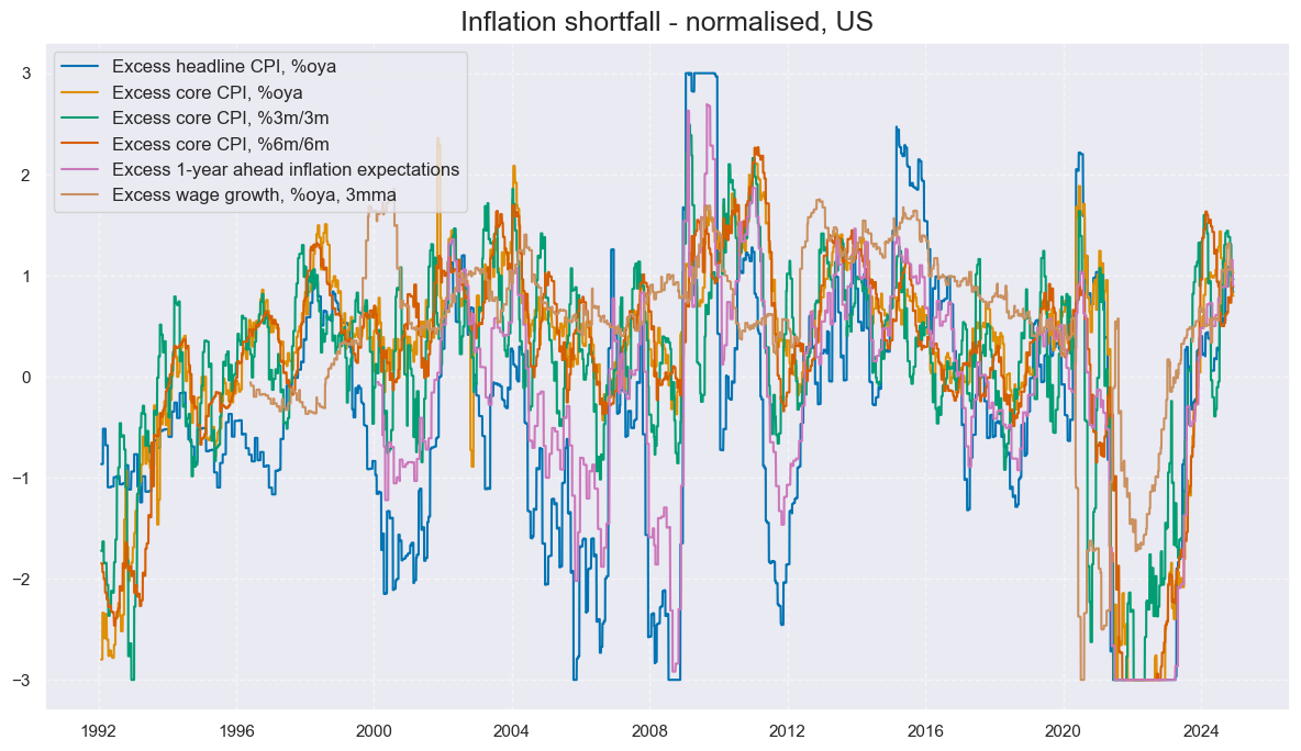
cidx = cids_gb
xcatx = [key + "_ZN" for key in list(dict_xinf.keys())]
labs = ['Excess headline CPI, %oya', 'Excess core CPI, %oya', 'Excess core CPI, %3m/3m', 'Excess core CPI, %6m/6m',
 'Excess 1-year ahead inflation expectations', 'Excess wage growth, %oya, 3mma']

msp.view_timelines(
    dfx,
    xcats=xcatx,
    cids=cidx,
    ncol=2,
    start="1992-01-01",
    same_y=True,
    title='Inflation shortfall - normalised, US',
    xcat_labels=labs
)
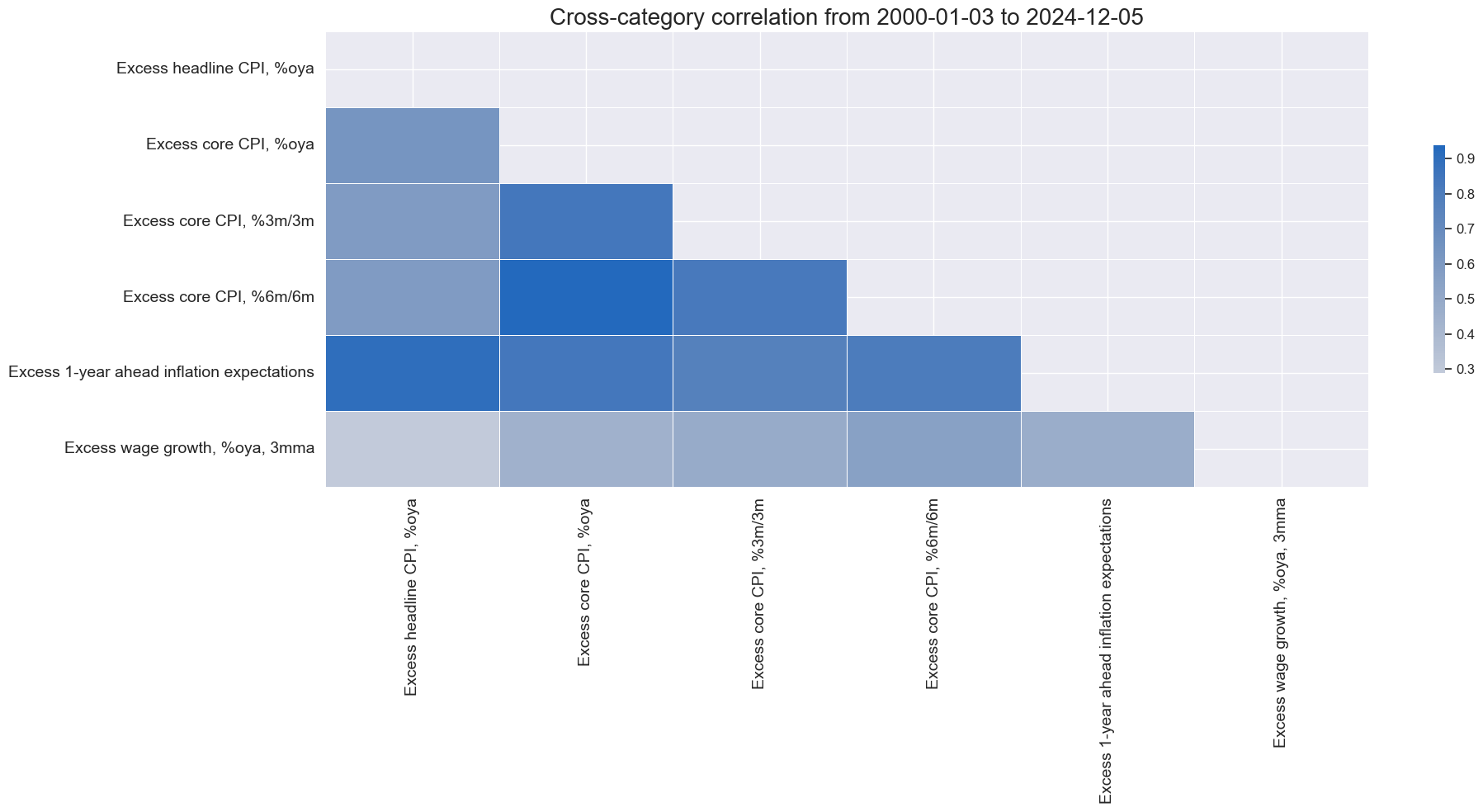
xcatx = [key + "_ZN" for key in list(dict_xinf.keys())]
cidx = cids_gb

msp.correl_matrix(
    dfx,
    xcats=xcatx,
    cids=cidx,
    freq="M",
    size=(20, 10),
    xcat_labels = labs,
)
Labor market slack #
# Transformations

cidx = cids_ecos

calcs = [
    "XEMPL_NSA_P1M1ML12_3MMA = EMPL_NSA_P1M1ML12_3MMA - WFORCE_NSA_P1Y1YL1_5YMM",  # relative to workforce growth
]
dfa = msp.panel_calculator(dfx, calcs=calcs, cids=cidx)
dfx = msm.update_df(dfx, dfa)
# Collect categories, labels, and presumed impact signs
cidx = cids_ecos
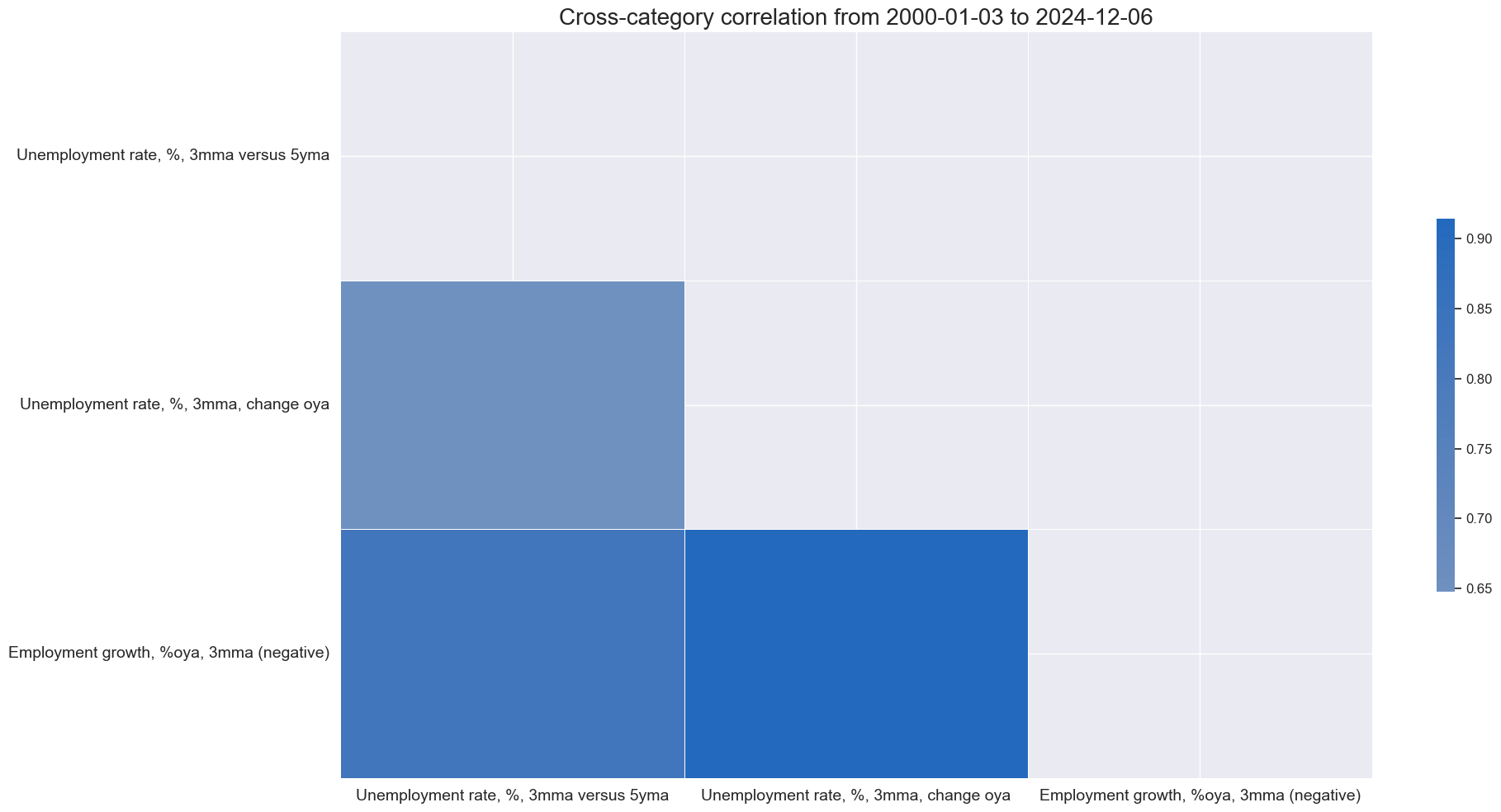
dict_base = {
"UNEMPLRATE_SA_3MMAv5YMA": "Unemployment rate, %, 3mma versus 5yma",
"UNEMPLRATE_NSA_3MMA_D1M1ML12": "Unemployment rate, %, 3mma, change oya",
"XEMPL_NSA_P1M1ML12_3MMA": "Employment growth, %oya, 3mma (negative)",
}
# Set correct signs for all categories and created amended dictionary
negs = [key for key, value in dict_base.items() if value.endswith("(negative)")]
calcs = []
for xc in negs:
calcs += [f"{xc}_NEG = - {xc}"]
dfa = msp.panel_calculator(dfx, calcs=calcs, cids=cidx)
dfx = msm.update_df(dfx, dfa)
keys_sa = [
key + "_NEG" if value.strip().endswith("(negative)") else key
for key, value in dict_base.items()
]
dict_labs = dict(zip(keys_sa, dict_base.values())) # dict with correct keys and labels
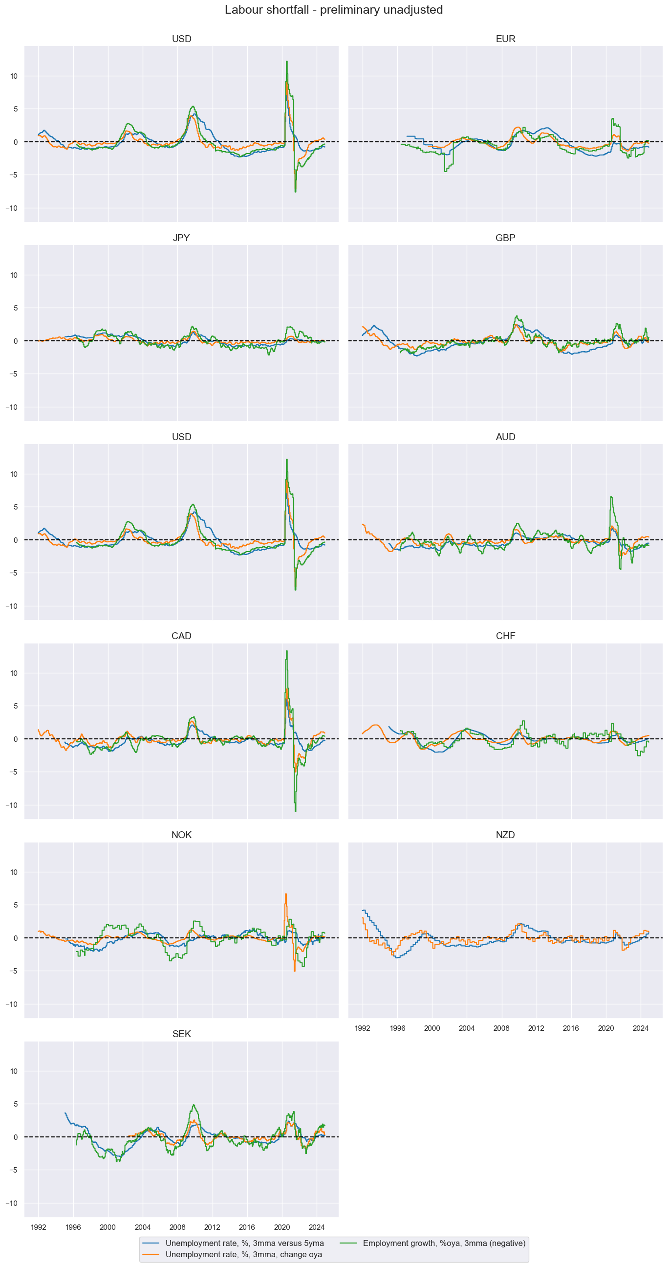
cidx = cids_ecos
xcatx = list(dict_labs.keys())

msp.view_timelines(
    dfx,
    xcats=xcatx,
    cids=cidx,
    ncol=2,
    start="1992-01-01",
    same_y=True,
    title='Labour shortfall - preliminary unadjusted',
    xcat_labels=list(dict_labs.values())
)
# Calculate standardized and winsorized values based on all countries

cidx = cids_ecos
xcatx = list(dict_labs.keys())
dfa = pd.DataFrame(columns=list(dfx.columns))

for xc in xcatx:
    dfaa = msp.make_zn_scores(
        dfx,
        xcat=xc,
        cids=cidx,
        sequential=True,
        min_obs=261 * 5,
        neutral="zero",
        pan_weight=1,
        thresh=3,
        postfix="_ZN",
        est_freq="m",
    )
    dfa = msm.update_df(dfa, dfaa)

dfx = msm.update_df(dfx, dfa)
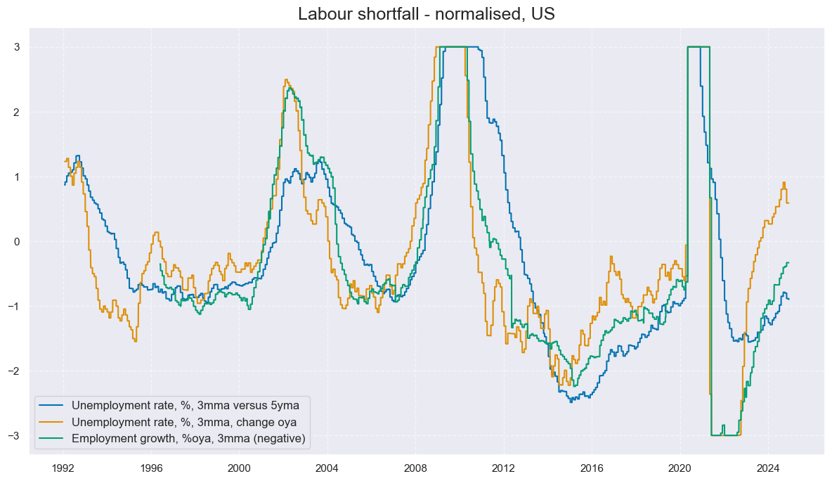
cidx = cids_gb
xcatx = [key + "_ZN" for key in list(dict_labs.keys())]
labs = list(dict_labs.values())

msp.view_timelines(
    dfx,
    xcats=xcatx,
    cids=cidx,
    ncol=2,
    start="1992-01-01",
    same_y=True,
    title='Labour shortfall - normalised, US',
    xcat_labels=labs
)
xcatx = [key + "_ZN" for key in list(dict_labs.keys())]
cidx = cids_gb

msp.correl_matrix(
    dfx,
    xcats=xcatx,
    cids=cidx,
    freq="M",
    size=(20, 10),
    xcat_labels = labs,
)
Growth and demand shortfall #
# Transformations
cidx = cids_ecos

calcs = [
    "XNRSALES_SA_P1M1ML12_3MMA = NRSALES_SA_P1M1ML12_3MMA - NGDP", # excess nominal retail sales
    "XIMPORTS_SA_P1M1ML12_3MMA = IMPORTS_SA_P1M1ML12_3MMA - NGDP", # Exces import growth
    "XRPCONS_SA_P1M1ML12_3MMA = RPCONS_SA_P1M1ML12_3MMA - RGDP_SA_P1Q1QL4_20QMM", # excess real private consumption
]
dfa = msp.panel_calculator(dfx, calcs=calcs, cids=cidx)
dfx = msm.update_df(dfx, dfa)
# Collect categories, labels, and presumed impact signs
cidx = cids_ecos
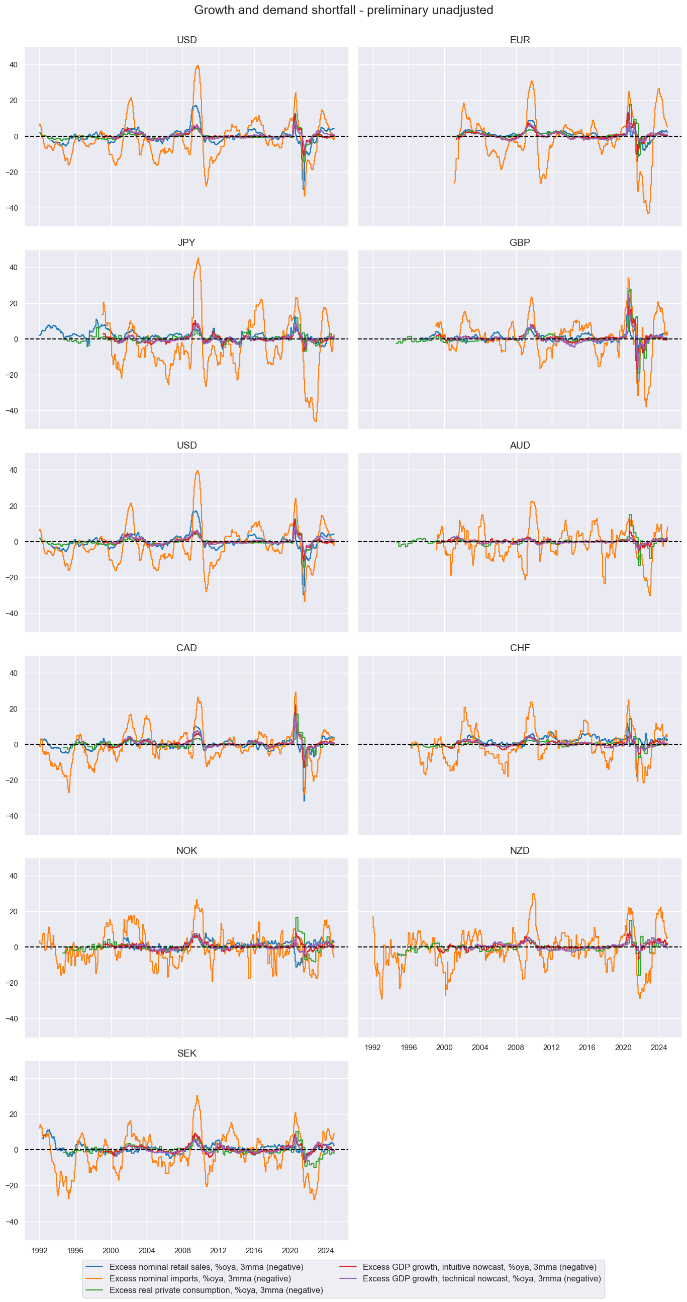
dict_base = {
"XNRSALES_SA_P1M1ML12_3MMA": "Excess nominal retail sales, %oya, 3mma (negative)",
"XIMPORTS_SA_P1M1ML12_3MMA": "Excess nominal imports, %oya, 3mma (negative)",
"XRPCONS_SA_P1M1ML12_3MMA": "Excess real private consumption, %oya, 3mma (negative)",
"INTRGDPv5Y_NSA_P1M1ML12_3MMA": "Excess GDP growth, intuitive nowcast, %oya, 3mma (negative)",
"RGDPTECHv5Y_SA_P1M1ML12_3MMA": "Excess GDP growth, technical nowcast, %oya, 3mma (negative)",
}
# Set correct signs for all categories and created amended dictionary
negs = [key for key, value in dict_base.items() if value.endswith("(negative)")]
calcs = []
for xc in negs:
calcs += [f"{xc}_NEG = - {xc}"]
dfa = msp.panel_calculator(dfx, calcs=calcs, cids=cidx)
dfx = msm.update_df(dfx, dfa)
keys_sa = [
key + "_NEG" if value.strip().endswith("(negative)") else key
for key, value in dict_base.items()
]
dict_xgds = dict(zip(keys_sa, dict_base.values())) # dict with correct keys and labels
cidx = cids_ecos
xcatx = list(dict_xgds.keys())
labs=list(dict_xgds.values())

msp.view_timelines(
    dfx,
    xcats=xcatx,
    cids=cidx,
    ncol=2,
    start="1992-01-01",
    same_y=True,
    title='Growth and demand shortfall - preliminary unadjusted',
    xcat_labels=labs
)
# Calculate standardized and winsorized values based on all countries

cidx = cids_ecos
xcatx = list(dict_xgds.keys())
dfa = pd.DataFrame(columns=list(dfx.columns))
labs = ['Excess nominal retail sales', 'Excess nominal imports', 'Excess real private consumption', 'Excess GDP growth, intuitive nowcast',
 'Excess GDP growth, technical nowcast']

for xc in xcatx:
    dfaa = msp.make_zn_scores(
        dfx,
        xcat=xc,
        cids=cidx,
        sequential=True,
        min_obs=261 * 5,
        neutral="zero",
        pan_weight=1,
        thresh=3,
        postfix="_ZN",
        est_freq="m",
    )
    dfa = msm.update_df(dfa, dfaa)

dfx = msm.update_df(dfx, dfa)
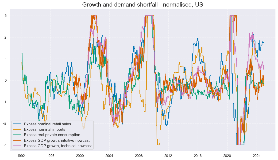
cidx = ["USD"]
xcatx = [key + "_ZN" for key in list(dict_xgds.keys())]
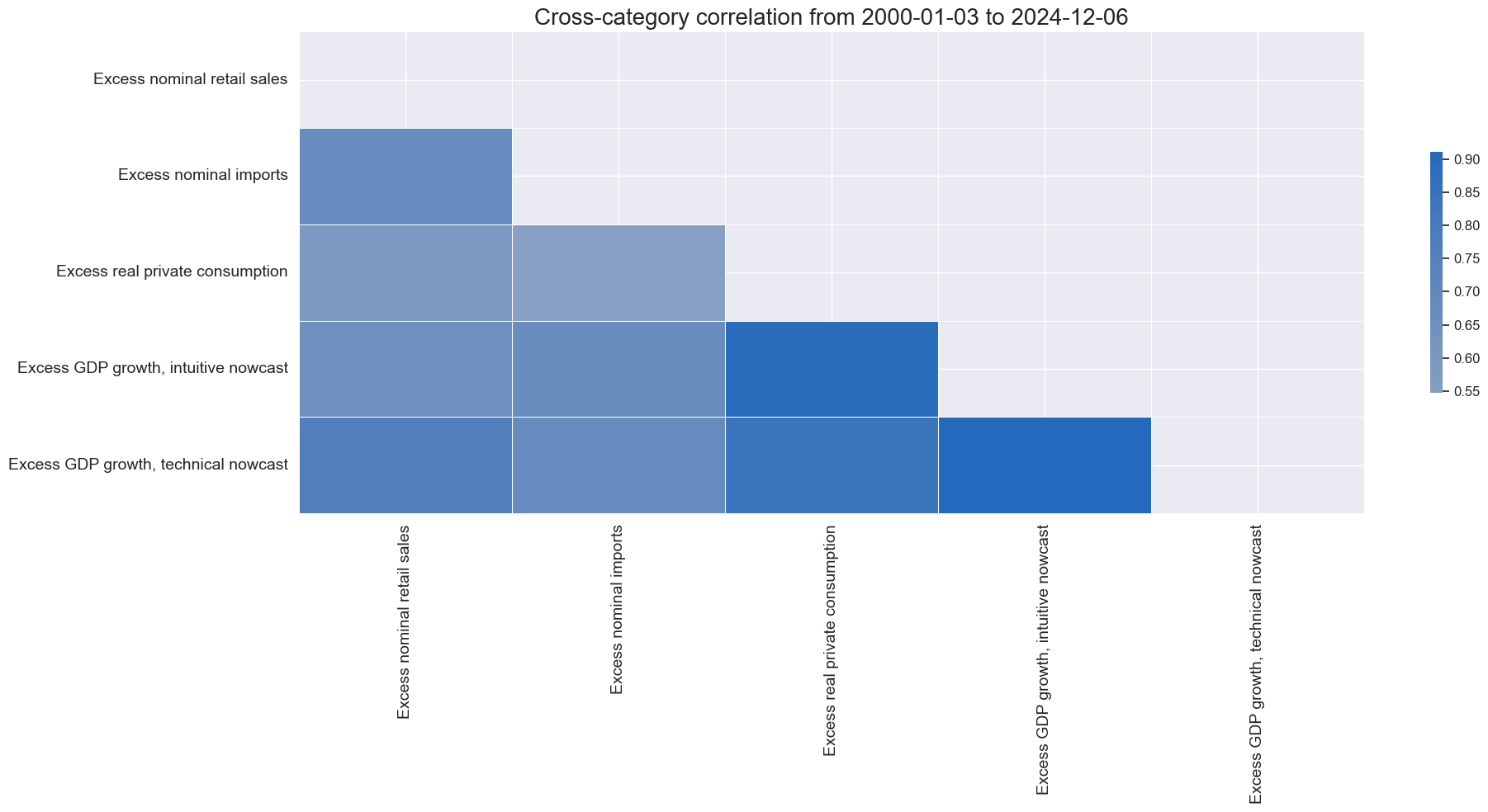
labs = [
"Excess nominal retail sales",
"Excess nominal imports",
"Excess real private consumption",
"Excess GDP growth, intuitive nowcast",
"Excess GDP growth, technical nowcast",
]
msp.view_timelines(
dfx,
xcats=xcatx,
cids=cidx,
ncol=2,
start="1992-01-01",
same_y=True,
title="Growth and demand shortfall - normalised, US",
xcat_labels=labs,
)
xcatx = [key + "_ZN" for key in list(dict_xgds.keys())]
cidx = cids_gb

msp.correl_matrix(
    dfx,
    xcats=xcatx,
    cids=cidx,
    freq="M",
    size=(20, 10),
    xcat_labels = labs,
)
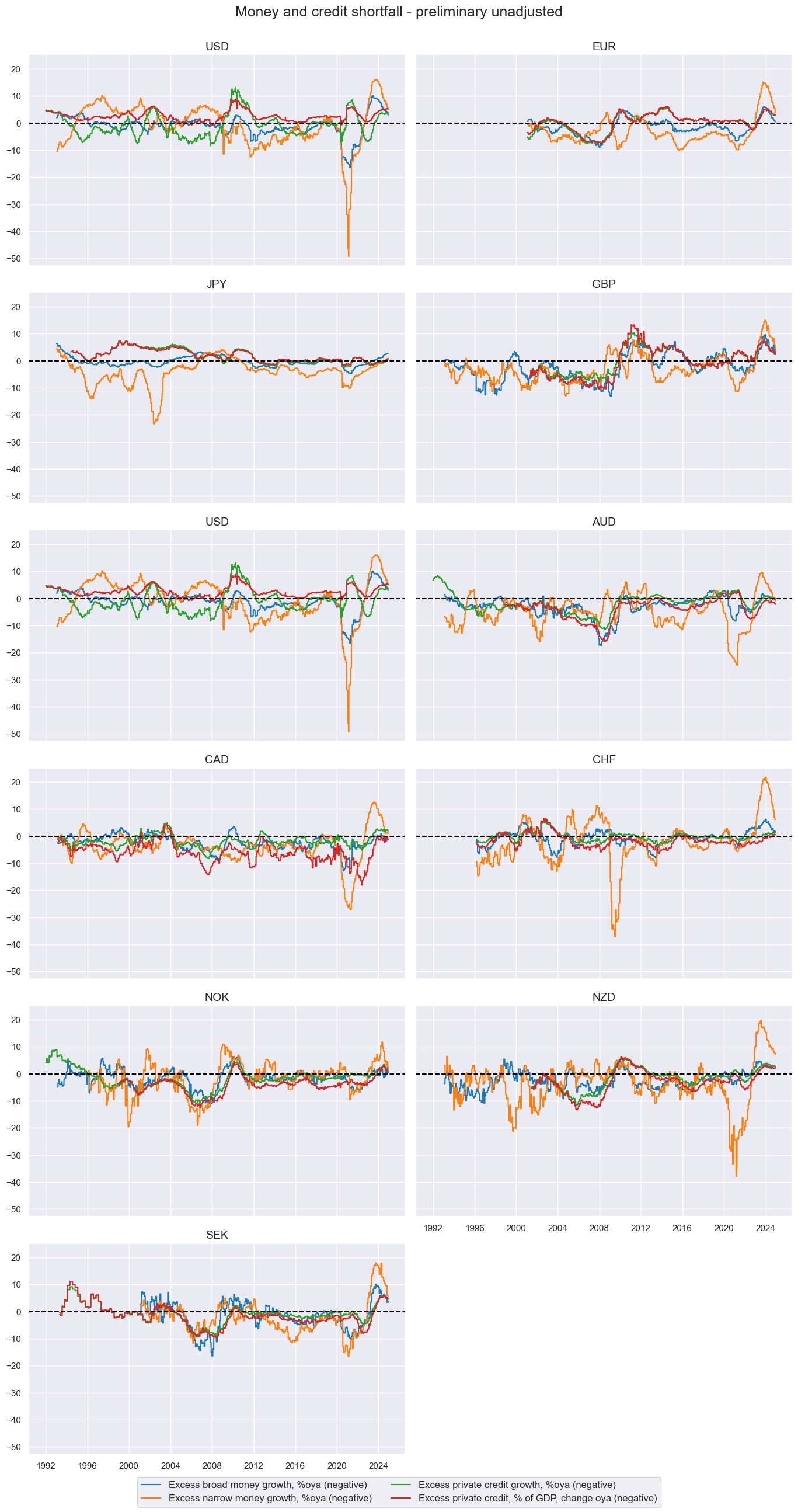
Money and credit shortfall #
# Transformations
cidx = cids_ecos

calcs = [
    # Excess money and credit growth
    "XMNARROW_SJA_P1M1ML12 = MNARROW_SJA_P1M1ML12 - NGDP",
    "XMBROAD_SJA_P1M1ML12 = MBROAD_SJA_P1M1ML12 - NGDP",
    "XPCREDITBN_SJA_P1M1ML12 = PCREDITBN_SJA_P1M1ML12 - NGDP",
    "XPCREDITGDP_SJA_D1M1ML12 = PCREDITGDP_SJA_D1M1ML12 - NGDP" # excess private bank credit
]
dfa = msp.panel_calculator(dfx, calcs=calcs, cids=cids)
dfx = msm.update_df(dfx, dfa)

xcred = list(dfa['xcat'].unique())
# Collect categories, labels, and presumed impact signs

cidx = cids_ecos
dict_base = {
    "XMBROAD_SJA_P1M1ML12": "Excess broad money growth, %oya (negative)",
    "XMNARROW_SJA_P1M1ML12": "Excess narrow money growth, %oya (negative)",
    "XPCREDITBN_SJA_P1M1ML12": "Excess private credit growth, %oya (negative)",
    "XPCREDITGDP_SJA_D1M1ML12": "Excess private credit, % of GDP, change oya (negative)",
}

# Set correct signs for all categories and created amended dictionary

negs = [key for key, value in dict_base.items() if value.endswith("(negative)")]

calcs = []
for xc in negs:
    calcs += [f"{xc}_NEG = - {xc}"]
dfa = msp.panel_calculator(dfx, calcs=calcs, cids=cidx)
dfx = msm.update_df(dfx, dfa)

keys_sa = [
    key + "_NEG" if value.strip().endswith("(negative)") else key
    for key, value in dict_base.items()
]

dict_mcrs = dict(zip(keys_sa, dict_base.values()))  # dict with correct keys and labels
cidx = cids_ecos
xcatx = list(dict_mcrs.keys())
labs = list(dict_mcrs.values())

msp.view_timelines(
    dfx,
    xcats=xcatx,
    cids=cidx,
    ncol=2,
    start="1992-01-01",
    same_y=True,
    title='Money and credit shortfall - preliminary unadjusted',
    xcat_labels=labs
)
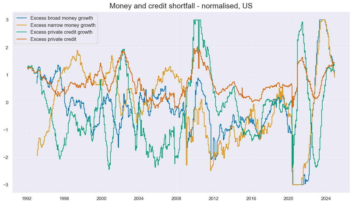
# Calculate standardized and winsorized values based on all countries

cidx = cids_ecos
xcatx = list(dict_mcrs.keys())
dfa = pd.DataFrame(columns=list(dfx.columns))
labs = ['Excess broad money growth', 'Excess narrow money growth', 'Excess private credit growth', 'Excess private credit']

for xc in xcatx:
    dfaa = msp.make_zn_scores(
        dfx,
        xcat=xc,
        cids=cidx,
        sequential=True,
        min_obs=261 * 5,
        neutral="zero",
        pan_weight=1,
        thresh=3,
        postfix="_ZN",
        est_freq="m",
    )
    dfa = msm.update_df(dfa, dfaa)

dfx = msm.update_df(dfx, dfa)
cidx = cids_gb
xcatx = [key + "_ZN" for key in list(dict_mcrs.keys())]

msp.view_timelines(
    dfx,
    xcats=xcatx,
    cids=cidx,
    ncol=2,
    start="1992-01-01",
    same_y=True,
    title='Money and credit shortfall - normalised, US',
    xcat_labels=labs
)
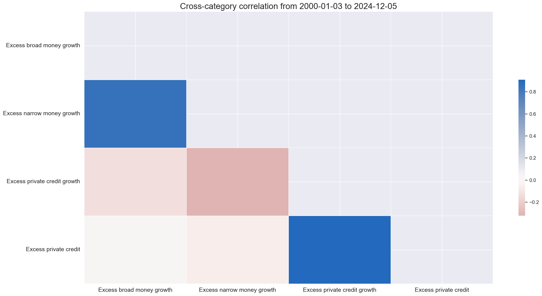
xcatx = [key + "_ZN" for key in list(dict_mcrs.keys())]
cidx = cids_gb

msp.correl_matrix(
    dfx,
    xcats=xcatx,
    cids=cidx,
    freq="M",
    size=(20, 10),
    xcat_labels = labs,
)
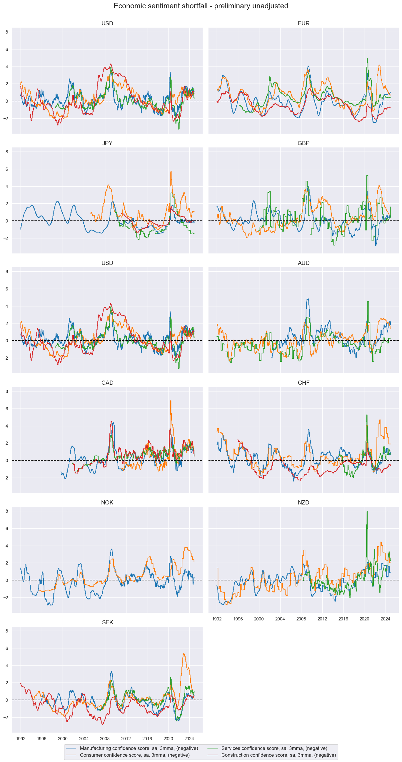
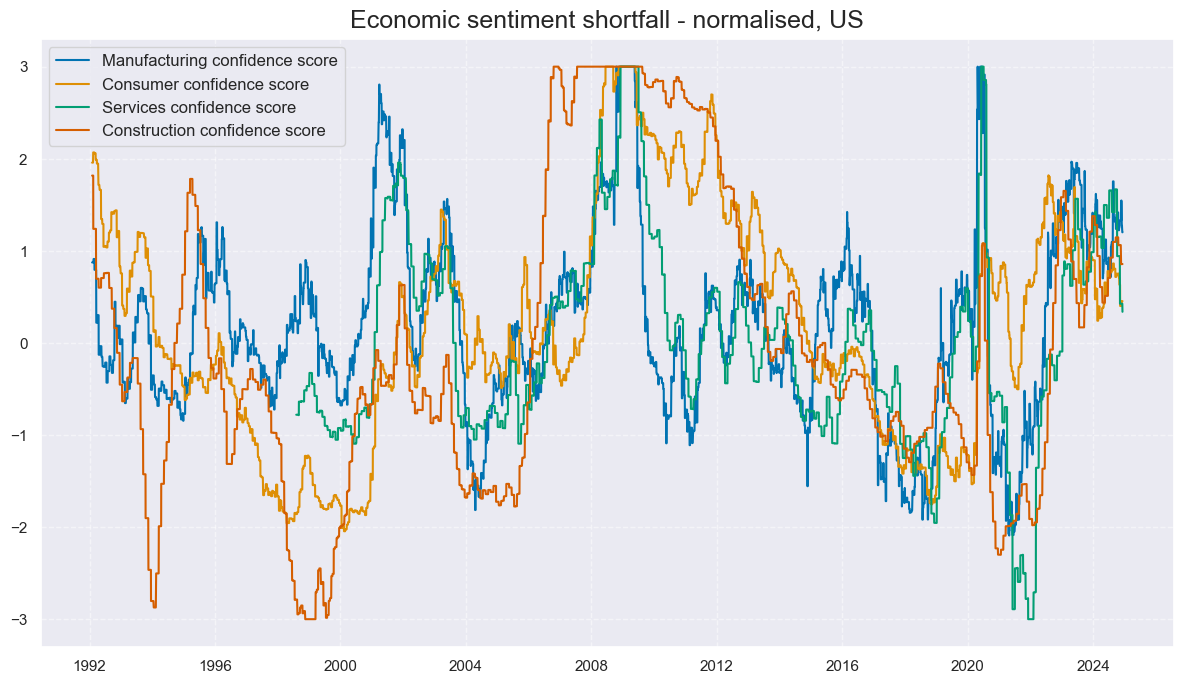
Economic sentiment shortfall #
# Collect categories, labels, and presumed impact signs

cidx = cids_ecos
dict_base = {
        "MBCSCORE_SA_3MMA": "Manufacturing confidence score, sa, 3mma, (negative)",
        "CCSCORE_SA_3MMA": "Consumer confidence score, sa, 3mma, (negative)",
        "SBCSCORE_SA_3MMA": "Services confidence score, sa, 3mma, (negative)",
        "CBCSCORE_SA_3MMA": "Construction confidence score, sa, 3mma, (negative)",
}

# Set correct signs for all categories and created amended dictionary

negs = [key for key, value in dict_base.items() if value.endswith("(negative)")]

calcs = []
for xc in negs:
    calcs += [f"{xc}_NEG = - {xc}"]
dfa = msp.panel_calculator(dfx, calcs=calcs, cids=cidx)
dfx = msm.update_df(dfx, dfa)

keys_sa = [
    key + "_NEG" if value.strip().endswith("(negative)") else key
    for key, value in dict_base.items()
]

dict_confs = dict(zip(keys_sa, dict_base.values()))  # dict with correct keys and labels
cidx = cids_ecos
xcatx = list(dict_confs.keys())
labs=list(dict_confs.values())

msp.view_timelines(
    dfx,
    xcats=xcatx,
    cids=cidx,
    ncol=2,
    start="1992-01-01",
    same_y=True,
    title='Economic sentiment shortfall - preliminary unadjusted',
    xcat_labels=labs
)
# Calculate standardized and winsorized values based on all countries

cidx = cids_ecos
xcatx = list(dict_confs.keys())
dfa = pd.DataFrame(columns=list(dfx.columns))
labs = ['Manufacturing confidence score', 'Consumer confidence score', 'Services confidence score', 'Construction confidence score']

for xc in xcatx:
    dfaa = msp.make_zn_scores(
        dfx,
        xcat=xc,
        cids=cidx,
        sequential=True,
        min_obs=261 * 5,
        neutral="zero",
        pan_weight=1,
        thresh=3,
        postfix="_ZN",
        est_freq="m",
    )
    dfa = msm.update_df(dfa, dfaa)

dfx = msm.update_df(dfx, dfa)
cidx = cids_gb
xcatx = [key + "_ZN" for key in list(dict_confs.keys())]

msp.view_timelines(
    dfx,
    xcats=xcatx,
    cids=cidx,
    ncol=2,
    start="1992-01-01",
    same_y=True,
    title='Economic sentiment shortfall - normalised, US',
    xcat_labels=labs
)
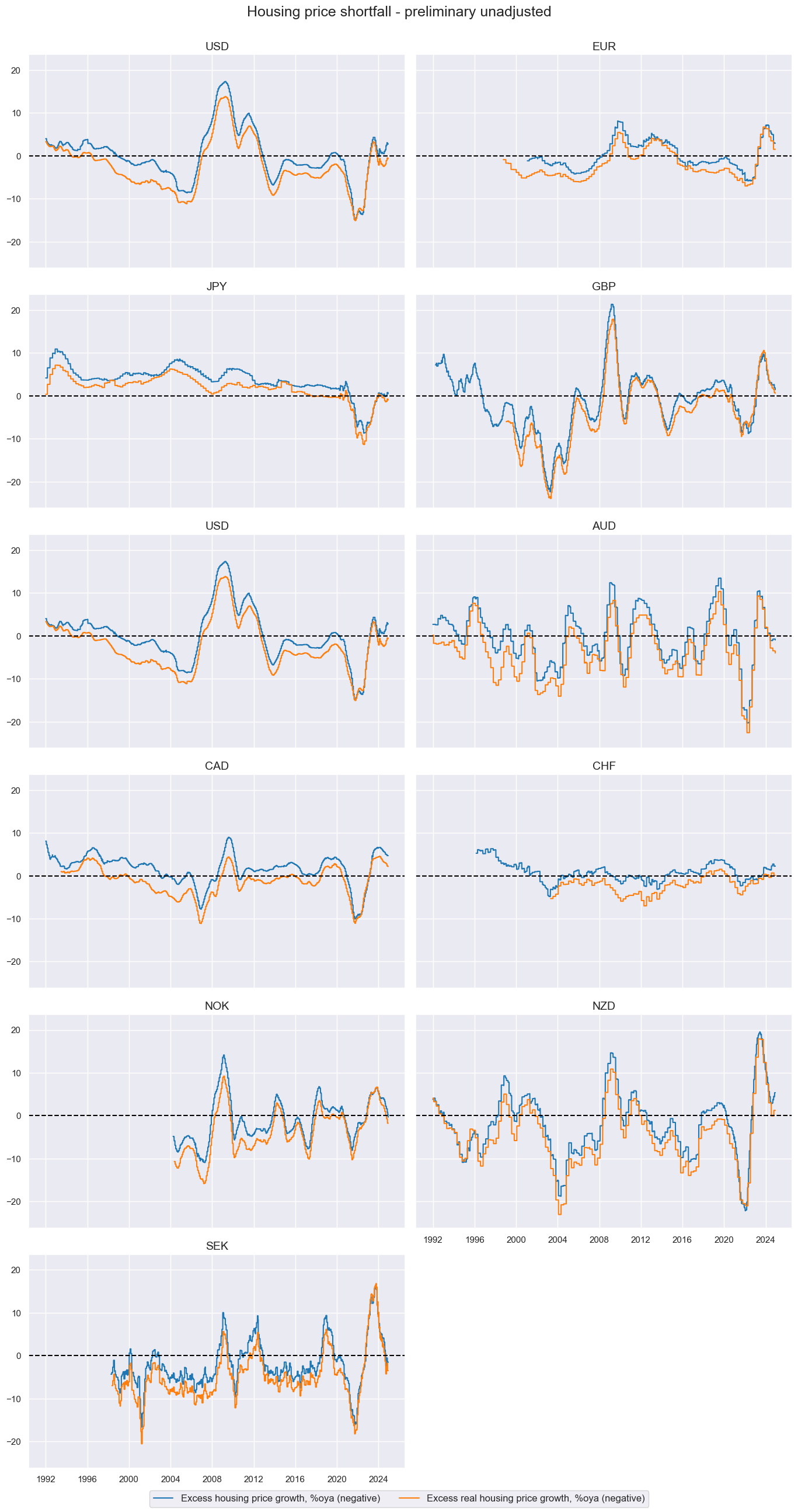
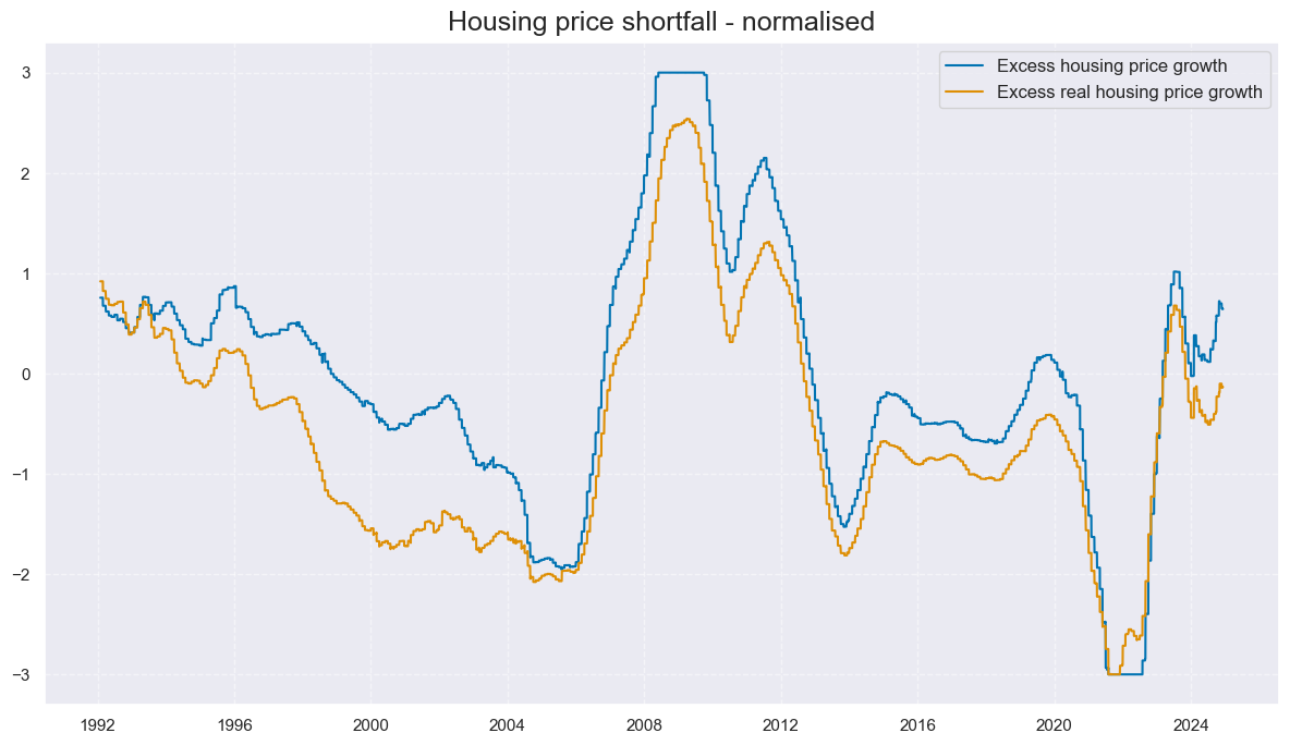
Housing price shortfall #
# Transformations

cidx = cids_ecos
calcs = ["XHPI_SA_P1M1ML12_3MMA = HPI_SA_P1M1ML12_3MMA - NGDP "] # excess house price growth]

dfa = msp.panel_calculator(dfx, calcs=calcs, cids=cidx)
dfx = msm.update_df(dfx, dfa)
# Collect categories, labels, and presumed impact signs

cidx = cids_ecos
dict_base = {
    "XHPI_SA_P1M1ML12_3MMA": "Excess housing price growth, %oya (negative)",
    "RHPI_SA_P1M1ML12_3MMA": "Excess real housing price growth, %oya (negative)",
}

# Set correct signs for all categories and created amended dictionary

negs = [key for key, value in dict_base.items() if value.endswith("(negative)")]

calcs = []
for xc in negs:
    calcs += [f"{xc}_NEG = - {xc}"]
dfa = msp.panel_calculator(dfx, calcs=calcs, cids=cidx)
dfx = msm.update_df(dfx, dfa)

keys_sa = [
    key + "_NEG" if value.strip().endswith("(negative)") else key
    for key, value in dict_base.items()
]

dict_hpis = dict(zip(keys_sa, dict_base.values()))  # dict with correct keys and labels
cidx = cids_ecos
xcatx = list(dict_hpis.keys())
labs=list(dict_hpis.values())

msp.view_timelines(
    dfx,
    xcats=xcatx,
    cids=cidx,
    ncol=2,
    start="1992-01-01",
    same_y=True,
    title='Housing price shortfall - preliminary unadjusted',
    xcat_labels=labs
)
# Calculate standardized and winsorized values based on all countries

cidx = cids_ecos
xcatx = list(dict_hpis.keys())
dfa = pd.DataFrame(columns=list(dfx.columns))

for xc in xcatx:
    dfaa = msp.make_zn_scores(
        dfx,
        xcat=xc,
        cids=cidx,
        sequential=True,
        min_obs=261 * 5,
        neutral="zero",
        pan_weight=1,
        thresh=3,
        postfix="_ZN",
        est_freq="m",
    )
    dfa = msm.update_df(dfa, dfaa)

dfx = msm.update_df(dfx, dfa)
cidx = cids_gb
xcatx = [key + "_ZN" for key in list(dict_hpis.keys())]
labs=['Excess housing price growth', 'Excess real housing price growth']

msp.view_timelines(
    dfx,
    xcats=xcatx,
    cids=cidx,
    ncol=2,
    start="1992-01-01",
    same_y=True,
    title='Housing price shortfall - normalised',
    xcat_labels=labs
)
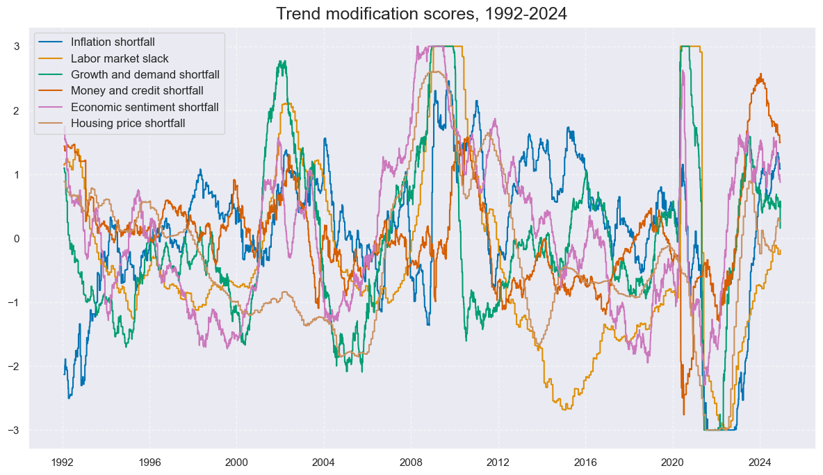
Trend modification scores #
Conceptual macro scores #
cidx = cids_ecos

dict_all = {
    "INFSHORT": [dict_xinf, "Inflation shortfall"],
    "LABSLACK": [dict_labs, "Labor market slack"],
    "GRDSHORT": [dict_xgds, "Growth and demand shortfall"],
    "MCRSHORT": [dict_mcrs, "Money and credit shortfall"],
    "SENTSHORT": [dict_confs, "Economic sentiment shortfall"],
    "HPISHORT": [dict_hpis, "Housing price shortfall"],
}
dict_labels = {key: value[1] for key, value in dict_all.items()}

dfa = pd.DataFrame(columns=list(dfx.columns))

for key, value in dict_all.items():
    xcatx = [key + "_ZN" for key in list(value[0].keys())]
    dfa1 = msp.linear_composite(
        df=dfx, xcats=xcatx, cids=cidx, complete_xcats=False, new_xcat=key
    )
    dfa2 = msp.make_zn_scores(
        dfa1,
        xcat=key,
        cids=cidx,
        sequential=True,
        min_obs=261 * 5,
        neutral="zero",
        pan_weight=1,
        thresh=3,
        postfix="_ZN",
        est_freq="m",
    )
    dfa = msm.update_df(dfa, dfa2)

dfx = msm.update_df(dfx, dfa)
cidx = cids_gb
xcatx = [key + "_ZN" for key in list(dict_all.keys())]

msp.view_timelines(
    dfx,
    xcats=xcatx,
    cids=cidx,
    ncol=2,
    start="1992-01-01",
    same_y=True,
    title='Trend modification scores, 1992-2024',
    xcat_labels=list(dict_labels.values())
)
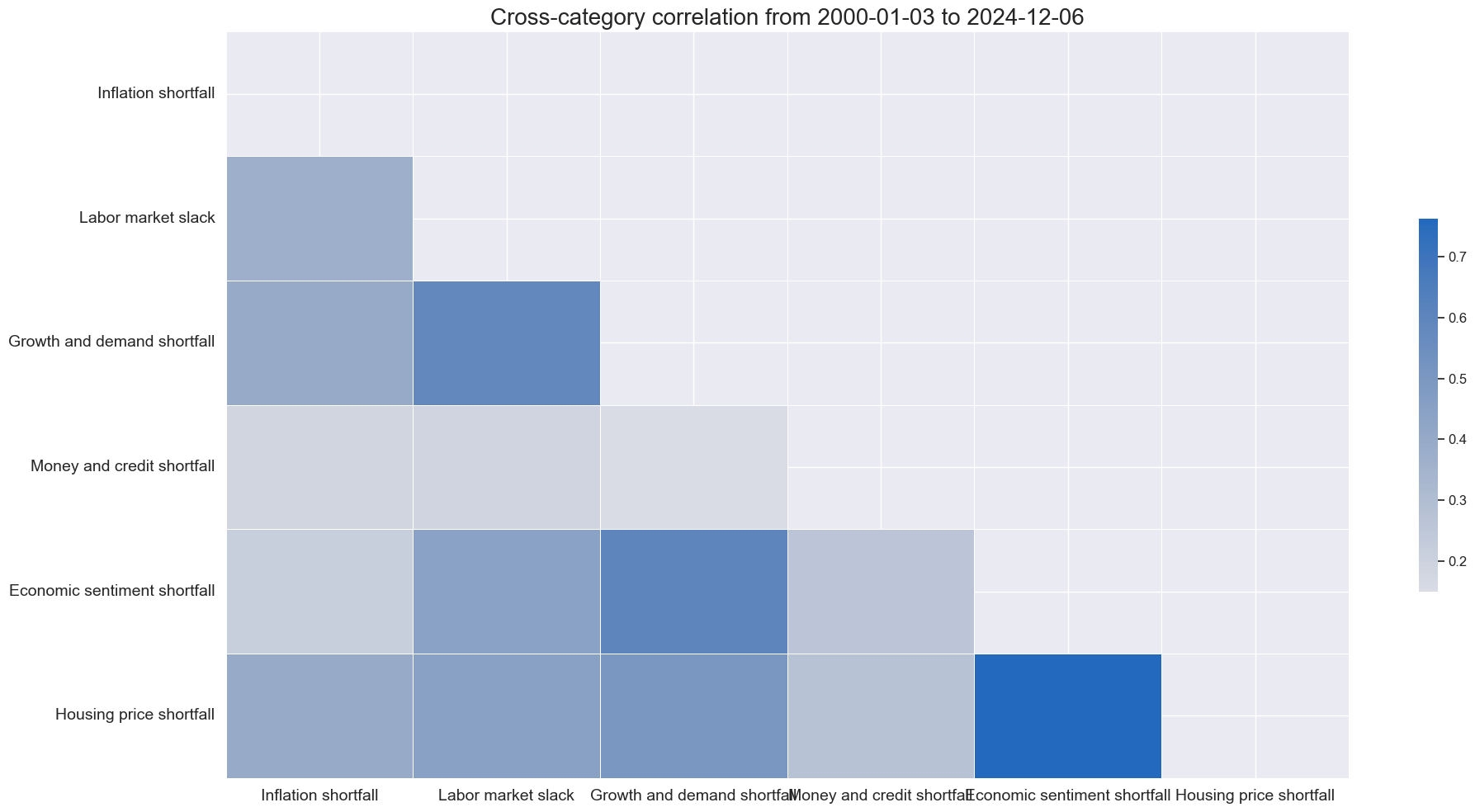
xcatx = [key + "_ZN" for key in list(dict_all.keys())]
cidx = cids_gb

msp.correl_matrix(
    dfx,
    xcats=xcatx,
    cids=cidx,
    freq="M",
    size=(20, 10),
    xcat_labels = list(dict_labels.values()),
)
Composite macro scores #
cidx = cids_ecos
xcatx = [key + "_ZN" for key in dict_all.keys()]
dfa1 = msp.linear_composite(
        df=dfx, xcats=xcatx, cids=cidx, complete_xcats=False, new_xcat="ALL_CZS"
    )
dfa2 = msp.make_zn_scores(
        dfa1,
        xcat="ALL_CZS",
        cids=cidx,
        sequential=True,
        min_obs=261 * 5,
        neutral="zero",
        pan_weight=1,
        thresh=3,
        postfix="_ZN",
        est_freq="m",
    )

dfx = msm.update_df(dfx, dfa2)
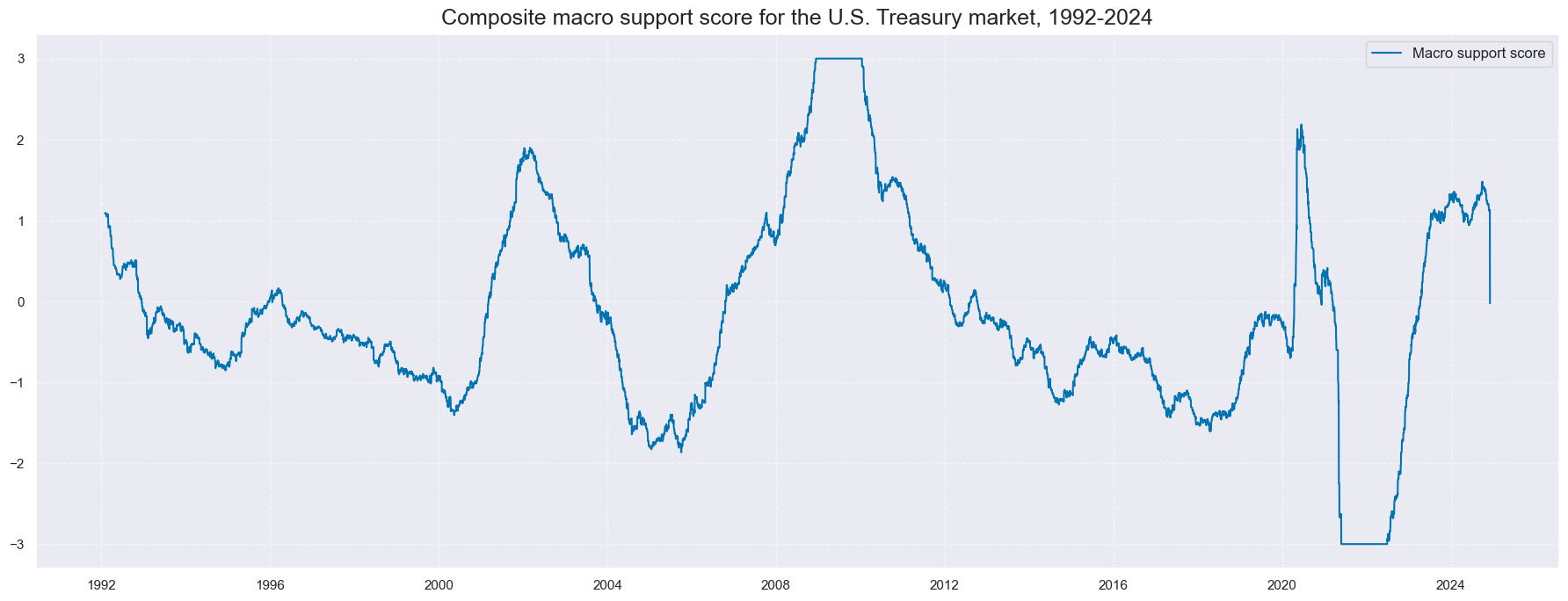
cidx = cids_gb
xcatx = ["ALL_CZS_ZN"]

msp.view_timelines(
    dfx,
    xcats=xcatx,
    cids=["USD"],
    start="1992-01-01",
    title="Composite macro support score for the U.S. Treasury market, 1992-2024",
    size=(18, 7),
    xcat_labels=['Macro support score']
)
# Negative score as convenience ticker for curve signal

cidx = cids_ecos
xcatx = [key + "_ZN" for key in dict_all.keys()] + ["ALL_CZS_ZN",]

dfa = pd.DataFrame(columns=list(dfx.columns))
for xc in xcatx:
    calcs = [
        f"{xc}_NEG = - {xc} ",
    ]
    dfaa = msp.panel_calculator(dfx, calcs=calcs, cids=cidx)
    dfa = msm.update_df(dfa, dfaa)

dfx = msm.update_df(dfx, dfa)
Return trends and adjustments #
Modified bond trends #
calcs = [
    # Moving Cumulative rets 5-year
    "GB05YXR_NSAI = GB05YXR_NSA.cumsum()",
    "GB05YXR_STMAV = GB05YXR_NSAI.rolling(20).mean()",
    "GB05YXR_LTMAV = GB05YXR_NSAI.rolling(100).mean()",
    # 2s10s
    "GB10v2VTXR = GB10YXR_VT10 - GB02YXR_VT10 ",
    "GB10v2VTXRCUM = GB10v2VTXR.cumsum()",
    "GB10v2VTXR_STMAV = GB10v2VTXRCUM.rolling(50).mean()",
    "GB10v2VTXR_LTMAV = GB10v2VTXRCUM.rolling(200).mean()",
    # Trends
    "GB05YXR_TREND = GB05YXR_STMAV - GB05YXR_LTMAV",
    "GB10v02YXR_TREND = GB10v2VTXR_STMAV - GB10v2VTXR_LTMAV",
]
dfa = msp.panel_calculator(dfx, calcs=calcs, cids=cids)
dfx = msm.update_df(dfx, dfa)
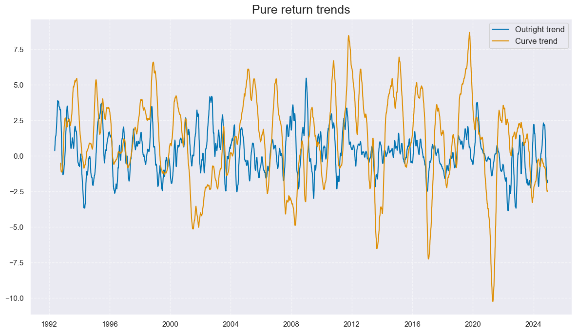
cidx = cids_gb
xcatx = ["GB05YXR_TREND", "GB10v02YXR_TREND"]

msp.view_timelines(
    dfx,
    xcats=xcatx,
    cids=cidx,
    ncol=2,
    start="1992-01-01",
    same_y=True,
    title='Pure return trends',
    xcat_labels=['Outright trend','Curve trend']
)
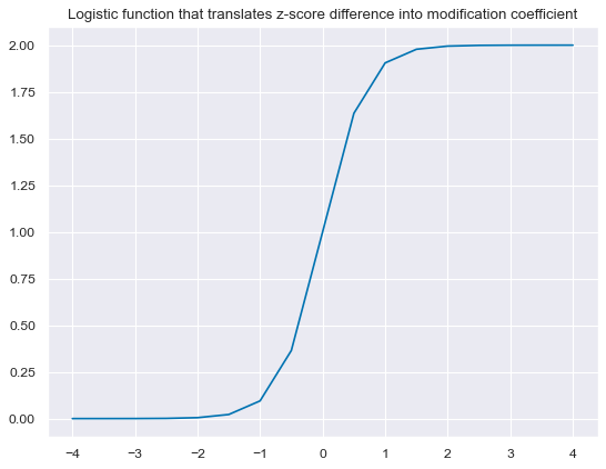
def sigmoid(x):
    return 2 / (1 + np.exp(-3 * x))

ar = np.array([i/2 for i in range(-8, 9)])
plt.figure(figsize=(8, 6), dpi=80)
plt.plot(ar, sigmoid(ar))
plt.title(
    "Logistic function that translates z-score difference into modification coefficient"
)
plt.show()
cidx = cids_gb
calcs = [
    f"ALL_WIND = 2 / (1 + np.exp( - 3 * ALL_CZS_ZN )) ",
    f"ALL_DIR_ADF = (1 - np.sign( GB05YXR_TREND )) + np.sign( GB05YXR_TREND ) * ALL_WIND ",
    f"ALL_CRV_ADF = (1 - np.sign( GB10v02YXR_TREND )) + np.sign( GB10v02YXR_TREND ) * ( 2 - ALL_WIND )  ",
    f"GB05YXR_MODTREND_ALL = GB05YXR_TREND * ALL_DIR_ADF ",
    f"GB10v02YXR_MODTREND_ALL = GB10v02YXR_TREND * ALL_CRV_ADF ",
]
dfa = msp.panel_calculator(dfx, calcs=calcs, cids=cidx)
dfx = msm.update_df(dfx, dfa)
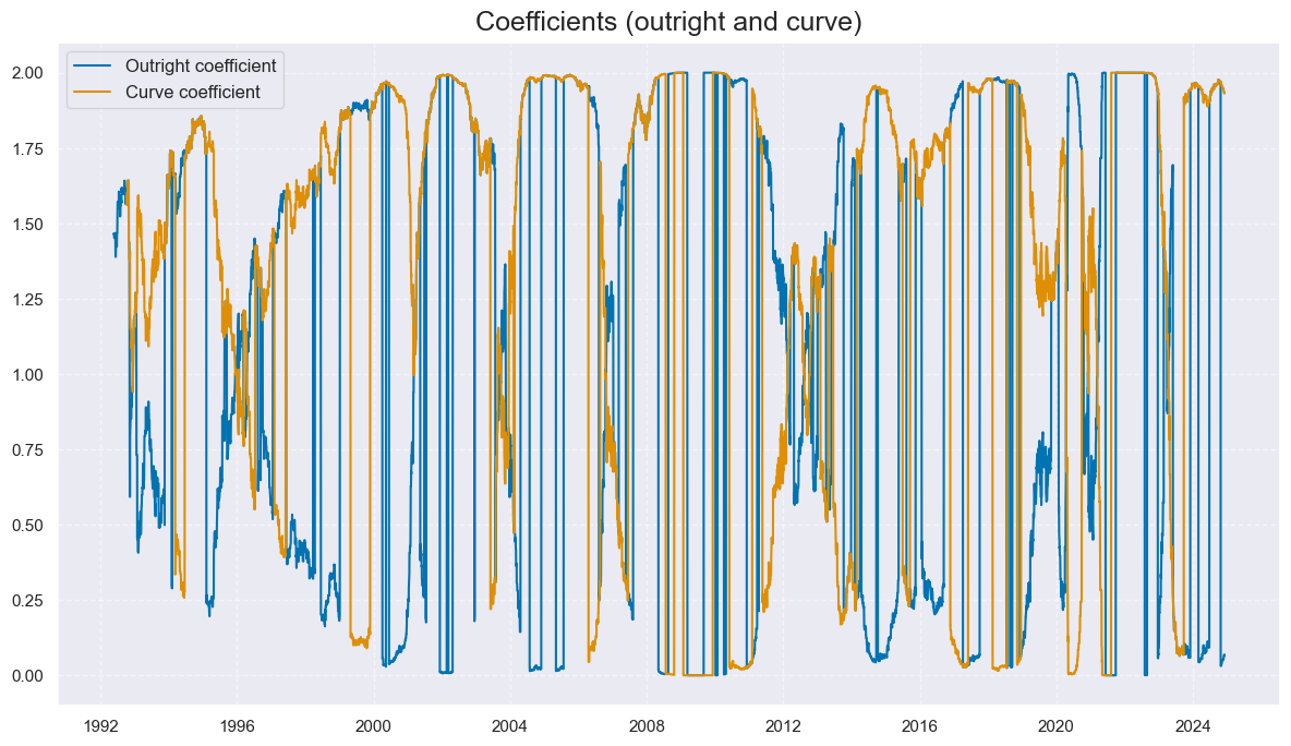
cidx = cids_gb
xcatx = ["ALL_DIR_ADF", "ALL_CRV_ADF"]

msp.view_timelines(
    dfx,
    xcats=xcatx,
    cids=cidx,
    ncol=2,
    start="1992-01-01",
    same_y=True,
    title='Coefficients (outright and curve)',
    xcat_labels=['Outright coefficient','Curve coefficient']
)
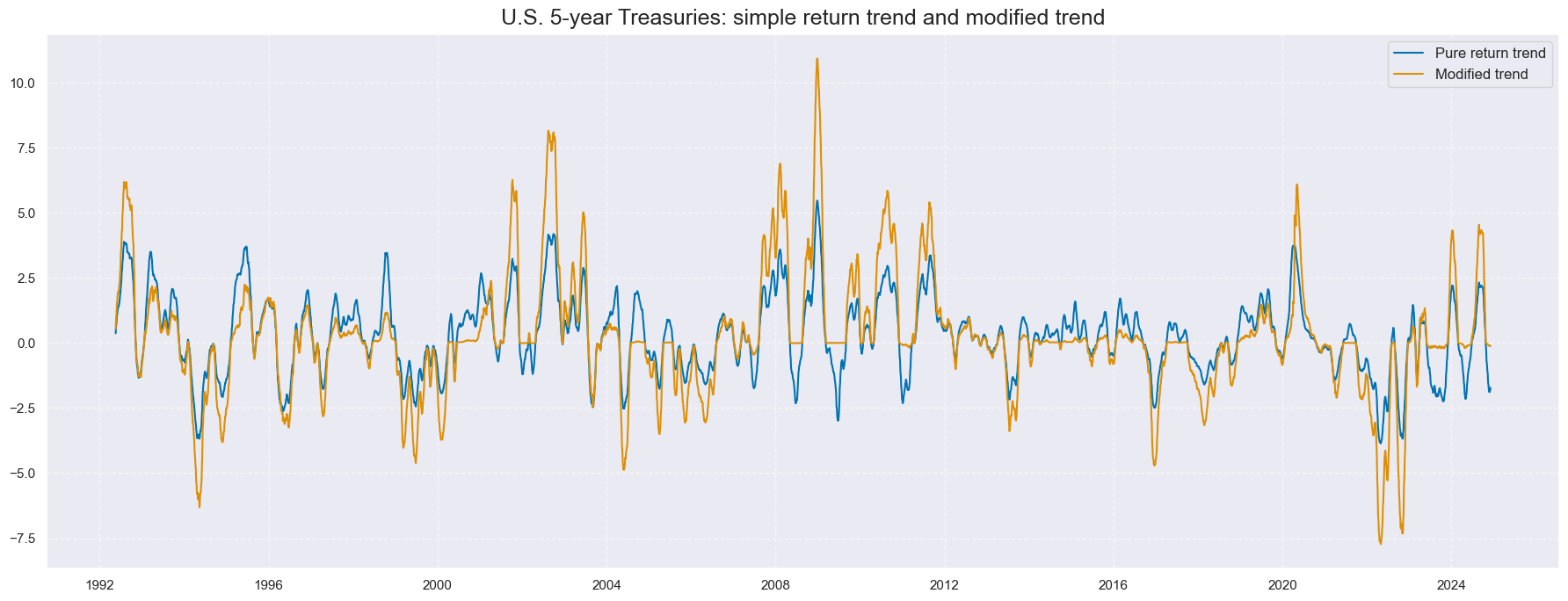
cidx = cids_gb
xcatx = ["GB05YXR_TREND", "GB05YXR_MODTREND_ALL"]

msp.view_timelines(
    dfx,
    xcats=xcatx,
    cids=cidx,
    start="1992-01-01",
    title="U.S. 5-year Treasuries: simple return trend and modified trend",
    size=(18, 7),
   xcat_labels=["Pure return trend", "Modified trend"],
)
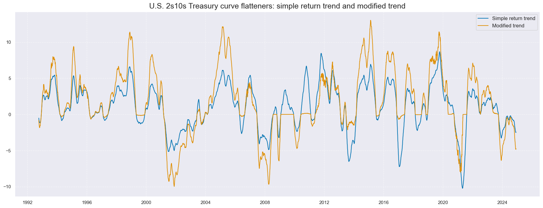
cidx = cids_gb
xcatx = ["GB10v02YXR_TREND", "GB10v02YXR_MODTREND_ALL"]

msp.view_timelines(
    dfx,
    xcats=xcatx,
    cids=cidx,
    start="1992-01-01",
    title="U.S. 2s10s Treasury curve flatteners: simple return trend and modified trend",
    size=(18, 7),
    xcat_labels=["Simple return trend", "Modified trend"],
)
# Normalization (mainly for comparability in charts)

xcatx = ["GB05YXR_MODTREND_ALL", "GB10v02YXR_MODTREND_ALL"]
cidx = cids_gb

dfa = pd.DataFrame(columns=list(dfx.columns))

for xc in xcatx:
    dfaa = msp.make_zn_scores(
        dfx,
        xcat=xc,
        cids=cidx,
        sequential=True,
        min_obs=261 * 5,
        neutral="zero",
        pan_weight=0,  # use country history
        thresh=3,
        postfix="_ZN",
        est_freq="m",
    )
    dfa = msm.update_df(dfa, dfaa)

dfx = msm.update_df(dfx, dfa)
Balanced bond trends #
xcatx = ['GB05YXR_TREND', 'GB10v02YXR_TREND']
cidx = cids_gb

dfa = pd.DataFrame(columns=list(dfx.columns))

for xc in xcatx:
    dfaa = msp.make_zn_scores(
        dfx,
        xcat=xc,
        cids=cidx,
        sequential=True,
        min_obs=261 * 5,
        neutral="zero",
        pan_weight=0,  # use country history
        thresh=3,
        postfix="_ZN",
        est_freq="m",
    )
    dfa = msm.update_df(dfa, dfaa)

dfx = msm.update_df(dfx, dfa)
cidx = cids_gb

xcatx = ["GB05YXR_TREND_ZN", "ALL_CZS_ZN"]
dfa1 = msp.linear_composite(
    df=dfx, xcats=xcatx, cids=cidx, complete_xcats=True, new_xcat="GB05YXR_BALTREND_ALL"
)
dfx = msm.update_df(dfx, dfa1)

xcatx = ["GB10v02YXR_TREND_ZN", "ALL_CZS_ZN"]
dfa2 = msp.linear_composite(
    df=dfx,
    xcats=xcatx,
    cids=cidx,
    signs=[1, -1],
    complete_xcats=True,
    new_xcat="GB10v02YXR_BALTREND_ALL",
)
dfx = msm.update_df(dfx, dfa2)
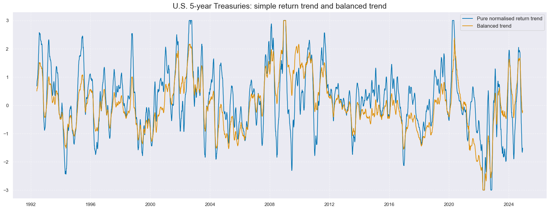
cidx = cids_gb
xcatx = ["GB05YXR_TREND_ZN", "GB05YXR_BALTREND_ALL"]

msp.view_timelines(
    dfx,
    xcats=xcatx,
    cids=cidx,
    start="1992-01-01",
    title="U.S. 5-year Treasuries: simple return trend and balanced trend",
    size=(18, 7),
    xcat_labels=["Pure normalised return trend", "Balanced trend"],
)
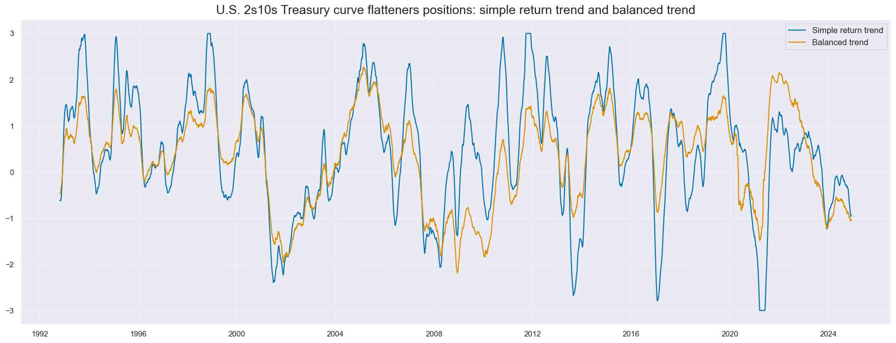
cidx = cids_gb
xcatx = ["GB10v02YXR_TREND_ZN", "GB10v02YXR_BALTREND_ALL"]

msp.view_timelines(
    dfx,
    xcats=xcatx,
    cids=cidx,
    start="1992-01-01",
    title="U.S. 2s10s Treasury curve flatteners positions: simple return trend and balanced trend",
    size=(18, 7),
    xcat_labels=["Simple return trend", "Balanced trend"],
)
Relations between trends #
Outright trends #
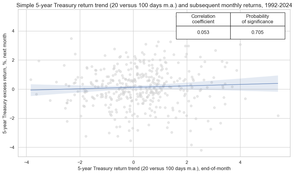
cidx = cids_gb
sig = 'GB05YXR_TREND'
ret = 'GB05YXR_NSA'

crx_mat = msp.CategoryRelations(
    dfx,
    xcats=[sig, ret],
    cids=cidx,
    freq="M",
    lag=1,
    xcat_aggs=["last", "sum"]
)
crx_mat.reg_scatter(
    labels=False,
    coef_box="upper right",
    title='Simple 5-year Treasury return trend (20 versus 100 days m.a.) and subsequent monthly returns, 1992-2024',
    size=(10, 6),
    xlab="5-year Treasury return trend (20 versus 100 days m.a.), end-of-month",
    ylab="5-year Treasury excess return, %, next month",
)
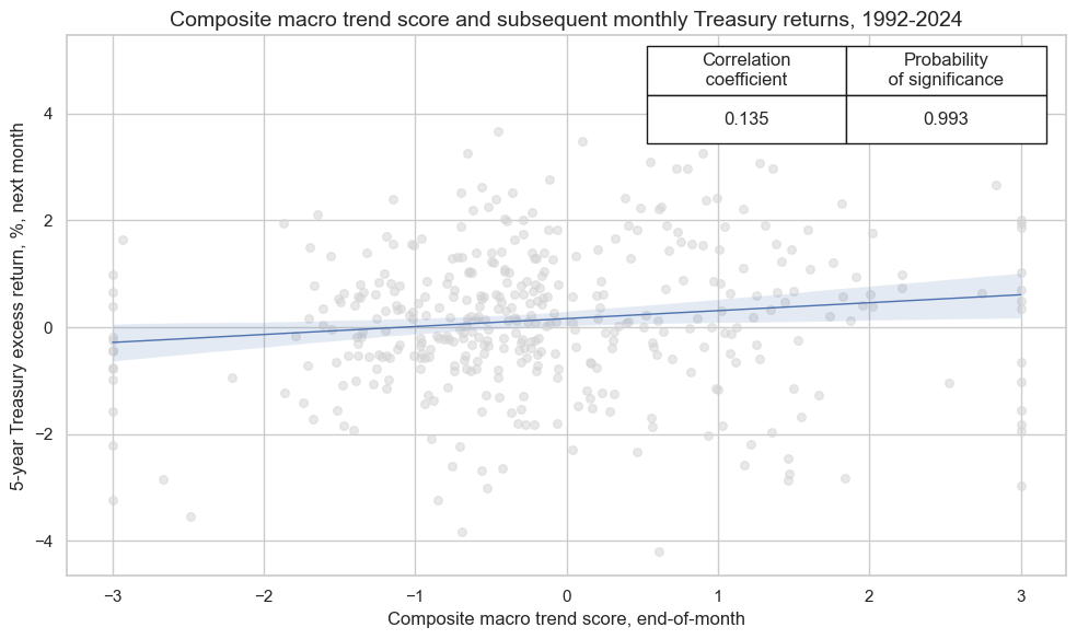
cidx = cids_gb
sig = 'ALL_CZS_ZN'
ret = 'GB05YXR_NSA'

crx_mat = msp.CategoryRelations(
    dfx,
    xcats=[sig, ret],
    cids=cidx,
    freq="M",
    lag=1,
    xcat_aggs=["last", "sum"]
)
crx_mat.reg_scatter(
    labels=False,
    coef_box="upper right",
    title='Composite macro trend score and subsequent monthly Treasury returns, 1992-2024',
    size=(10, 6),
    xlab="Composite macro trend score, end-of-month",
    ylab="5-year Treasury excess return, %, next month",
)
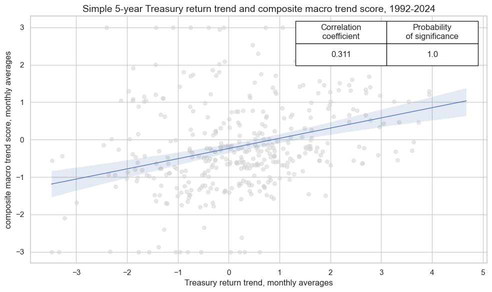
cidx = cids_gb
sig = 'GB05YXR_TREND'
ret = 'ALL_CZS_ZN'

crx_mat = msp.CategoryRelations(
    dfx,
    xcats=[sig, ret],
    cids=cidx,
    freq="M",
    lag=0,
    xcat_aggs=["mean", "mean"]
)
crx_mat.reg_scatter(
    labels=False,
    coef_box="upper right",
    title='Simple 5-year Treasury return trend and composite macro trend score, 1992-2024',
    size=(10, 6),
    prob_est="map",
    xlab="Treasury return trend, monthly averages",
    ylab="composite macro trend score, monthly averages",
)
Curve trends #
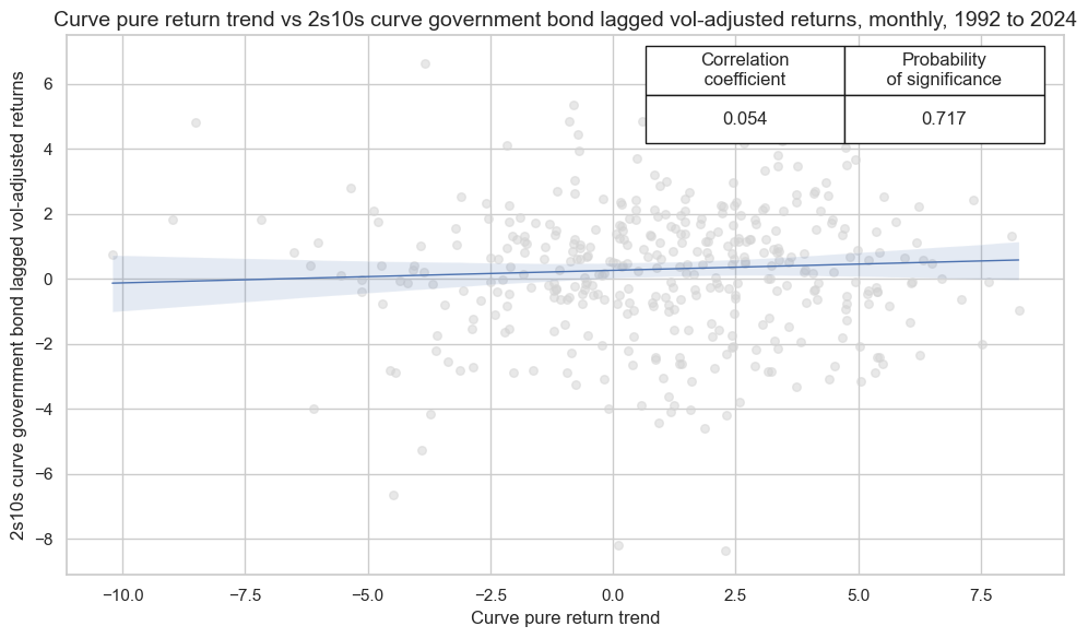
cidx = cids_gb
sig = 'GB10v02YXR_TREND'
ret = 'GB10v2VTXR'

crx_mat = msp.CategoryRelations(
    dfx,
    xcats=[sig, ret],
    cids=cidx,
    freq="M",
    lag=1,
    xcat_aggs=["last", "sum"]
)
crx_mat.reg_scatter(
    labels=False,
    coef_box="upper right",
    xlab="Curve pure return trend",
    ylab="2s10s curve government bond lagged vol-adjusted returns",
    title='Curve pure return trend vs 2s10s curve government bond lagged vol-adjusted returns, monthly, 1992 to 2024',
    size=(10, 6),
    prob_est="map",
)
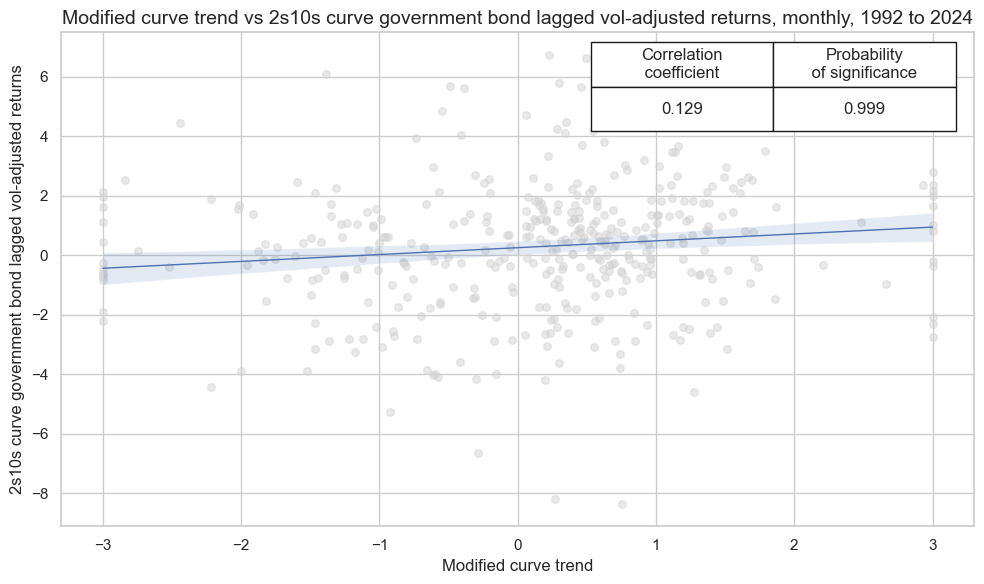
cidx = cids_gb
sig = 'ALL_CZS_ZN_NEG'
ret = 'GB10v2VTXR'

crx_mat = msp.CategoryRelations(
    dfx,
    xcats=[sig, ret],
    cids=cidx,
    freq="M",
    lag=1,
    xcat_aggs=["last", "sum"]
)
crx_mat.reg_scatter(
    labels=False,
    coef_box="upper right",
    xlab="Modified curve trend",
    ylab="2s10s curve government bond lagged vol-adjusted returns",
    title='Modified curve trend vs 2s10s curve government bond lagged vol-adjusted returns, monthly, 1992 to 2024',
    size=(10, 6),
    prob_est="map",
)
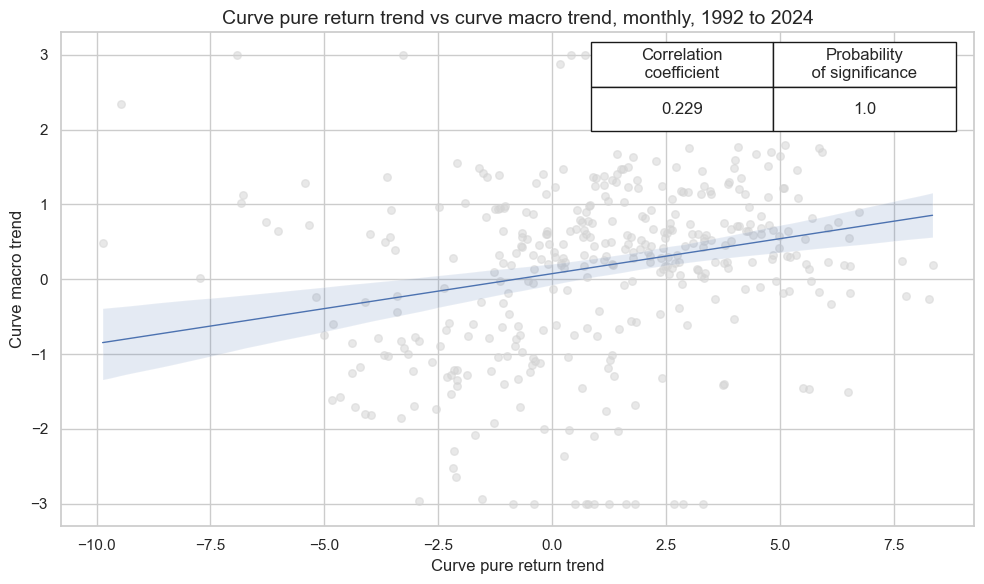
cidx = cids_gb
sig = 'GB10v02YXR_TREND'
ret = 'ALL_CZS_ZN_NEG'

crx_mat = msp.CategoryRelations(
    dfx,
    xcats=[sig, ret],
    cids=cidx,
    freq="M",
    lag=0,
    xcat_aggs=["mean", "mean"]
)
crx_mat.reg_scatter(
    labels=False,
    coef_box="upper right",
    xlab="Curve pure return trend",
    ylab="Curve macro trend",
    title='Curve pure return trend vs curve macro trend, monthly, 1992 to 2024',
    size=(10, 6),
    prob_est="map",
)
Value check #
Directional trend signals #
Specs and panel tests #
sigs = [
    "GB05YXR_TREND_ZN",
    "GB05YXR_MODTREND_ALL_ZN",
    "GB05YXR_BALTREND_ALL",
    "ALL_CZS_ZN",
]
targ = ["GB05YXR_NSA"]
cidx = cids_gb
start = "1992-01-01"

dict_dir = {
    "sigs": sigs,
    "targs": targ,
    "cidx": cidx,
    "start": start,
    "srr": None,
    "pnls": None,
}
dix = dict_dir
sigs = dix["sigs"]
targ = dix["targs"][0]
cidx = dix["cidx"]
start = dix["start"]
# Initialize the dictionary to store CategoryRelations instances
dict_cr = {}
for sig in sigs:
dict_cr[sig] = msp.CategoryRelations(
dfx,
xcats=[sig, targ],
cids=cidx,
freq="M",
lag=1,
xcat_aggs=["last", "sum"],
start=start,
)
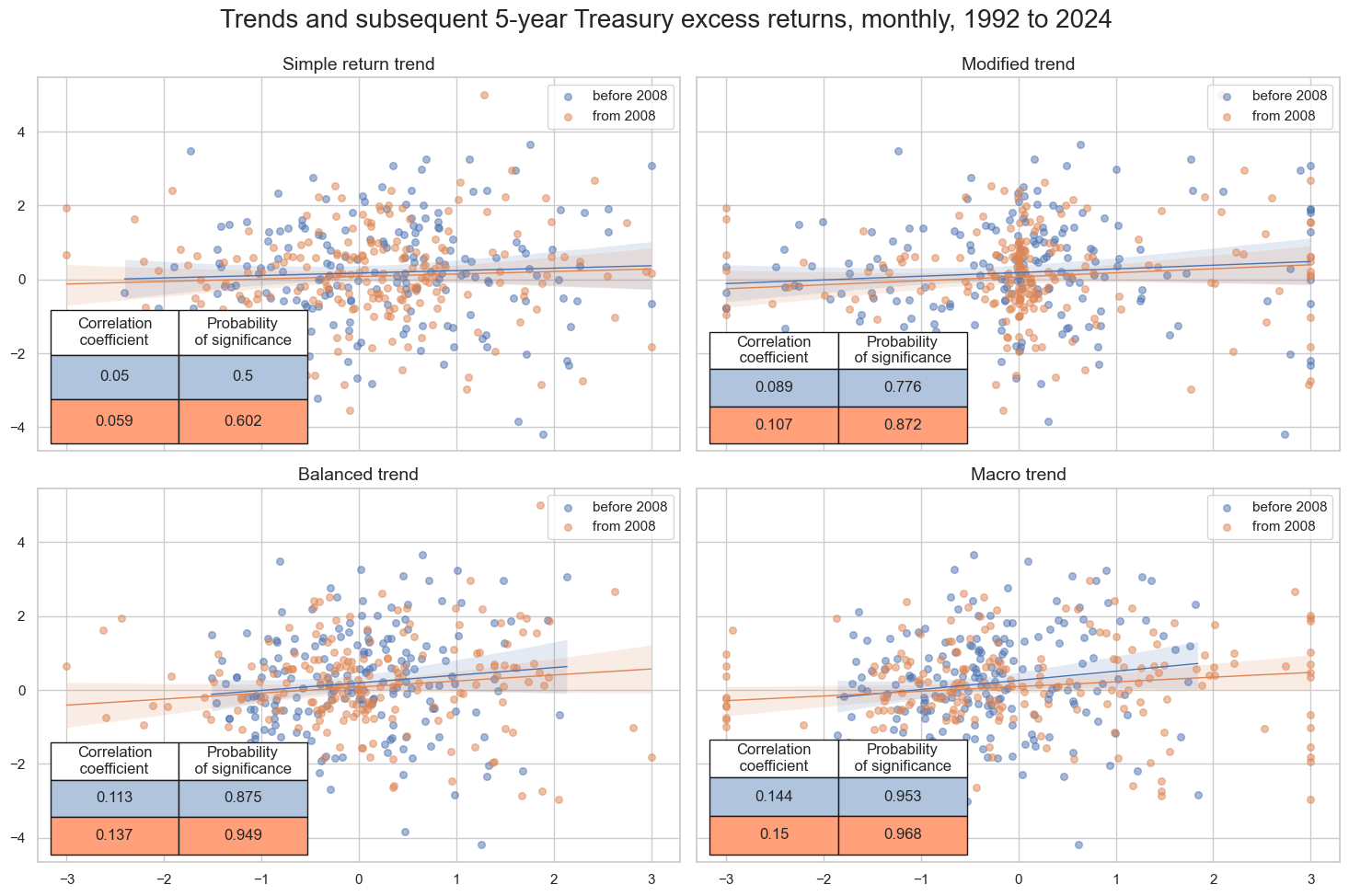
# Plotting the results
crs = list(dict_cr.values())
crs_keys = list(dict_cr.keys())
msv.multiple_reg_scatter(
cat_rels=crs,
title="Trends and subsequent 5-year Treasury excess returns, monthly, 1992 to 2024",
ylab=None,
ncol=2,
nrow=2,
separator=2008,
figsize=(15, 10),
prob_est="pool",
coef_box="lower left",
subplot_titles=[
"Simple return trend",
"Modified trend",
"Balanced trend",
"Macro trend",
],
)
Accuracy and correlation check #
dix = dict_dir

sigx = dix["sigs"]
targx = [dix["targs"][0]]
cidx = dix["cidx"]
start = dix["start"]

srr = mss.SignalReturnRelations(
    dfx,
    cids=cidx,
    sigs=sigx,
    rets=targx,
    freqs="M",
    start=start,
)

dix["srr"] = srr
dix = dict_dir
srr = dix["srr"]
srrx = srr.signals_table().reset_index()
srrx['Signal'] = srrx['Signal'].apply(lambda x: col_mapping.get(x, x))
srrx = srrx.set_index(['Return','Signal','Frequency','Aggregation'])
display(srrx.sort_index().astype("float").round(3))
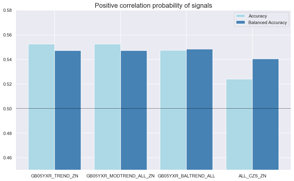
srr.accuracy_bars(
type="signals",
size=(14, 7),
title="Positive correlation probability of signals",
)
| accuracy | bal_accuracy | pos_sigr | pos_retr | pos_prec | neg_prec | pearson | pearson_pval | kendall | kendall_pval | auc | ||||
|---|---|---|---|---|---|---|---|---|---|---|---|---|---|---|
| Return | Signal | Frequency | Aggregation | |||||||||||
| GB05YXR_NSA | ALL_CZS_ZN | M | last | 0.524 | 0.540 | 0.359 | 0.547 | 0.599 | 0.482 | 0.135 | 0.007 | 0.097 | 0.004 | 0.538 |
| GB05YXR_BALTREND_ALL | M | last | 0.547 | 0.548 | 0.488 | 0.547 | 0.597 | 0.500 | 0.122 | 0.016 | 0.099 | 0.003 | 0.549 | |
| GB05YXR_MODTREND_ALL_ZN | M | last | 0.552 | 0.547 | 0.565 | 0.547 | 0.588 | 0.506 | 0.096 | 0.058 | 0.084 | 0.013 | 0.547 | |
| GB05YXR_TREND_ZN | M | last | 0.552 | 0.547 | 0.565 | 0.547 | 0.588 | 0.506 | 0.056 | 0.267 | 0.054 | 0.109 | 0.547 |

Naive PnL #
dix = dict_dir

sigx = dix["sigs"]
targ = dix["targs"][0]
cidx = dix["cidx"]
start = dix["start"]

naive_pnl = msn.NaivePnL(
    dfx,
    ret=targ,
    sigs=sigx,
    cids=cidx,
    start=start,
    bms=["USD_GB10YXR_NSA"],
)

for sig in sigx:
    for bias in [0, 1]:
        naive_pnl.make_pnl(
            sig,
            sig_neg=False,
            sig_op='zn_score_pan',
            sig_add=bias,
            thresh=3,
            rebal_freq="monthly",
            vol_scale=10,
            rebal_slip=1,
            pnl_name=sig+"_PZN" + str(bias)
        )

naive_pnl.make_long_pnl(vol_scale=10, label="Long only")

dix["pnls"] = naive_pnl
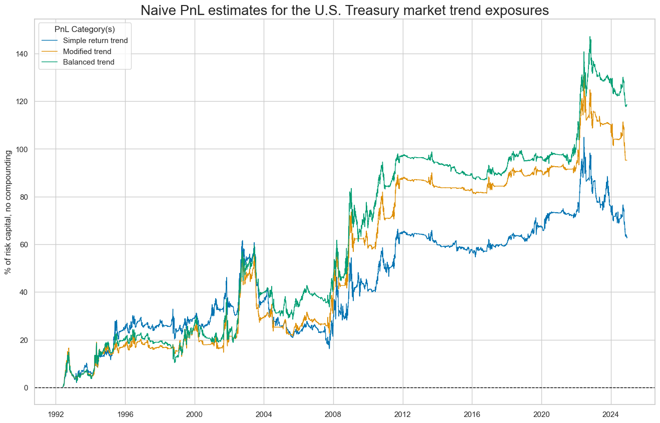
dix = dict_dir

sigx = dix["sigs"]
start = dix["start"]
cidx = dix["cidx"]
naive_pnl = dix["pnls"]

pnls = [sig + "_PZN0" for sig in sigx[:3]] # + ["Long only"]

naive_pnl.plot_pnls(
    pnl_cats=pnls,
    pnl_cids=["ALL"],
    start=start,
    title='Naive PnL estimates for the U.S. Treasury market trend exposures',
    xcat_labels=['Simple return trend','Modified trend','Balanced trend'],
    figsize=(16, 10),
)
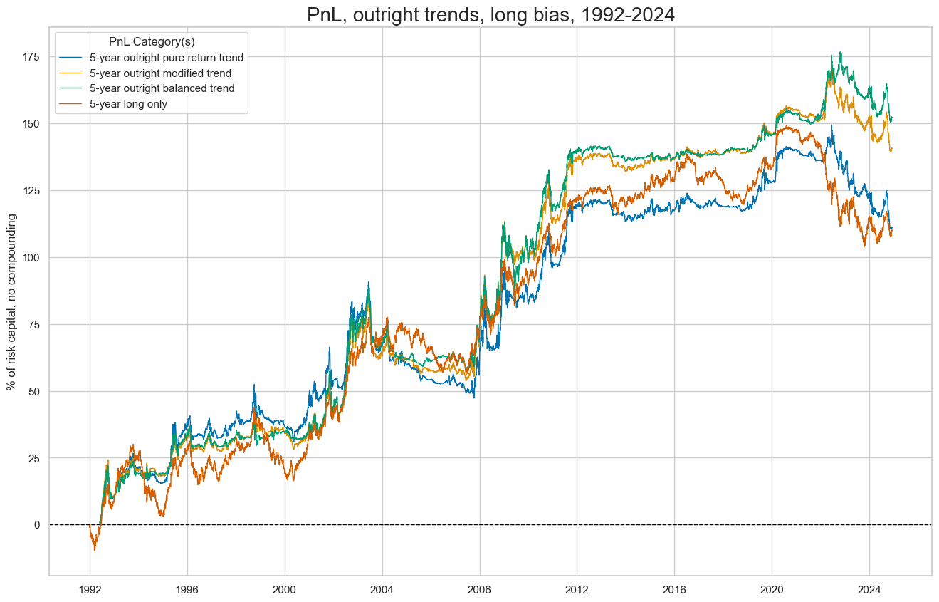
dix = dict_dir

sigx = dix["sigs"]
start = dix["start"]
cidx = dix["cidx"]
naive_pnl = dix["pnls"]

pnls = [sig + "_PZN1" for sig in sigx[:3]]  + ["Long only"]

naive_pnl.plot_pnls(
    pnl_cats=pnls,
    pnl_cids=["ALL"],
    start=start,
    title='PnL, outright trends, long bias, 1992-2024',
    xcat_labels=['5-year outright pure return trend','5-year outright modified trend','5-year outright balanced trend', '5-year long only'],
    figsize=(16, 10),
)
dix = dict_dir
sigx = dix["sigs"]
start = dix["start"]
cidx = dix["cidx"]
naive_pnl = dix["pnls"]
pnls = [s + "_PZN" + str(bias) for s in sigx for bias in [0, 1]] + ["Long only"]
df_eval = naive_pnl.evaluate_pnls(
pnl_cats=pnls,
pnl_cids=["ALL"],
start=start,
)
column_mapping = {
'ALL_CZS_ZN_PZN0': 'Macro trend',
'ALL_CZS_ZN_PZN1': 'Long macro trend',
'GB05YXR_BALTREND_ALL_PZN0': 'Balanced trend',
'GB05YXR_BALTREND_ALL_PZN1': 'Long balanced trend',
'GB05YXR_MODTREND_ALL_ZN_PZN0': 'Modified trend',
'GB05YXR_MODTREND_ALL_ZN_PZN1': 'Long modified trend',
'GB05YXR_TREND_ZN_PZN0': 'Pure trend',
'GB05YXR_TREND_ZN_PZN1': 'Long pure trend',
'Long only': 'Long only'
}
# Rename the columns
df_eval = df_eval.rename(columns=column_mapping)
display(df_eval.transpose())
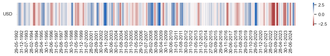
naive_pnl.signal_heatmap(
pnl_name=pnls[0],
freq="m",
title=None,
figsize=(15, 1)
)
| Return % | St. Dev. % | Sharpe Ratio | Sortino Ratio | Max 21-Day Draw % | Max 6-Month Draw % | Peak to Trough Draw % | Top 5% Monthly PnL Share | USD_GB10YXR_NSA correl | Traded Months | |
|---|---|---|---|---|---|---|---|---|---|---|
| xcat | ||||||||||
| Pure trend | 1.93269 | 10.0 | 0.193269 | 0.273418 | -14.47169 | -24.666536 | -45.449062 | 2.349345 | 0.173845 | 396 |
| Long pure trend | 3.412059 | 10.0 | 0.341206 | 0.485745 | -15.403989 | -24.662458 | -43.484261 | 1.431819 | 0.63065 | 396 |
| Modified trend | 2.930814 | 10.0 | 0.293081 | 0.419563 | -16.529002 | -26.829469 | -35.789243 | 1.755985 | 0.159116 | 396 |
| Long modified trend | 4.32908 | 10.0 | 0.432908 | 0.6219 | -15.312802 | -22.761292 | -34.150162 | 1.193194 | 0.593598 | 396 |
| Balanced trend | 3.644575 | 10.0 | 0.364457 | 0.527435 | -14.983569 | -20.564685 | -30.940448 | 1.373788 | 0.1602 | 396 |
| Long balanced trend | 4.68629 | 10.0 | 0.468629 | 0.670632 | -14.453283 | -23.917795 | -31.306809 | 1.04208 | 0.580924 | 396 |
| Macro trend | 3.622873 | 10.0 | 0.362287 | 0.521796 | -15.570546 | -28.652359 | -35.589481 | 1.33093 | 0.033457 | 396 |
| Long macro trend | 5.063123 | 10.0 | 0.506312 | 0.72456 | -14.93982 | -27.314174 | -29.118257 | 0.953295 | 0.471831 | 396 |
| Long only | 3.340665 | 10.0 | 0.334066 | 0.474767 | -10.115653 | -22.966953 | -45.295476 | 1.132314 | 0.919757 | 396 |
Curve trend signals #
Specs and panel tests #
sigs = [
    "GB10v02YXR_TREND_ZN",
    "GB10v02YXR_MODTREND_ALL_ZN",
    "GB10v02YXR_BALTREND_ALL",
    "ALL_CZS_ZN_NEG",
]
targ = ["GB10v2VTXR"]
cidx = cids_gb
start = "1992-01-01"

dict_crv = {
    "sigs": sigs,
    "targs": targ,
    "cidx": cidx,
    "start": start,
    "srr": None,
    "pnls": None,
}
dix = dict_crv
sigs = dix["sigs"]
targ = dix["targs"][0]
cidx = dix["cidx"]
start = dix["start"]
# Initialize the dictionary to store CategoryRelations instances
dict_cr = {}
for sig in sigs:
dict_cr[sig] = msp.CategoryRelations(
dfx,
xcats=[sig, targ],
cids=cidx,
freq="M",
lag=1,
xcat_aggs=["last", "sum"],
start=start,
)
# Plotting the results
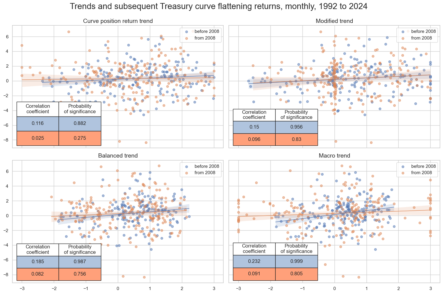
crs = list(dict_cr.values())
crs_keys = list(dict_cr.keys())
msv.multiple_reg_scatter(
cat_rels=crs,
title="Trends and subsequent Treasury curve flattening returns, monthly, 1992 to 2024",
ylab=None,
ncol=2,
nrow=2,
separator=2008,
figsize=(15, 10),
prob_est="pool",
coef_box="lower left",
subplot_titles=[
"Curve position return trend",
"Modified trend",
"Balanced trend",
"Macro trend",
],
)
Accuracy and correlation check #
dix = dict_crv

sigx = dix["sigs"]
targx = [dix["targs"][0]]
cidx = dix["cidx"]
start = dix["start"]

srr = mss.SignalReturnRelations(
    dfx,
    cids=cidx,
    sigs=sigx,
    rets=targx,
    freqs="M",
    start=start,
)

dix["srr"] = srr
dix = dict_crv
srr = dix["srr"]
srrx = srr.signals_table().reset_index()
srrx['Signal'] = srrx['Signal'].apply(lambda x: col_mapping.get(x, x))
srrx = srrx.set_index(['Return','Signal','Frequency','Aggregation'])
display(srrx.sort_index().astype("float").round(3))
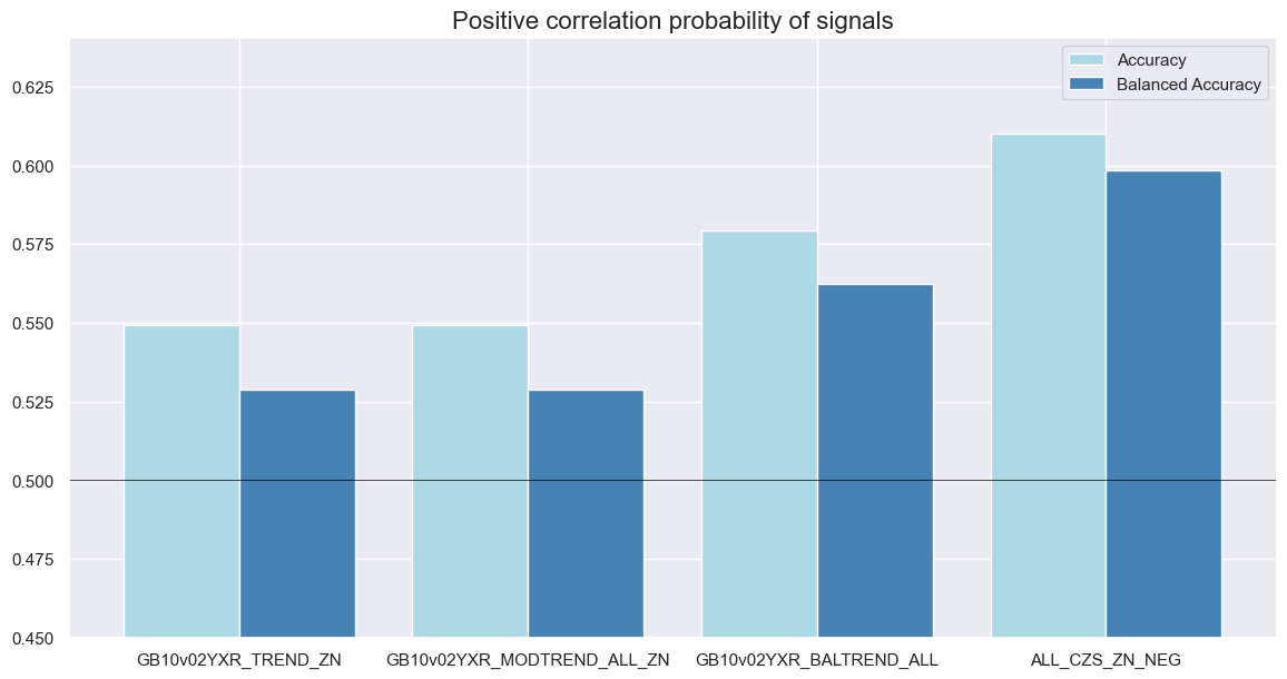
srr.accuracy_bars(
type="signals",
size=(14, 7),
title="Positive correlation probability of signals",
)
| accuracy | bal_accuracy | pos_sigr | pos_retr | pos_prec | neg_prec | pearson | pearson_pval | kendall | kendall_pval | auc | ||||
|---|---|---|---|---|---|---|---|---|---|---|---|---|---|---|
| Return | Signal | Frequency | Aggregation | |||||||||||
| GB10v2VTXR | Balanced trend | M | last | 0.579 | 0.562 | 0.665 | 0.571 | 0.613 | 0.512 | 0.120 | 0.018 | 0.077 | 0.024 | 0.557 |
| Macro trend | M | last | 0.610 | 0.598 | 0.641 | 0.570 | 0.640 | 0.556 | 0.129 | 0.010 | 0.109 | 0.001 | 0.592 | |
| Modified trend | M | last | 0.549 | 0.529 | 0.661 | 0.573 | 0.592 | 0.466 | 0.118 | 0.021 | 0.069 | 0.044 | 0.526 | |
| Pure return trend | M | last | 0.549 | 0.529 | 0.661 | 0.573 | 0.592 | 0.466 | 0.061 | 0.234 | 0.037 | 0.278 | 0.526 |
Naive PnL #
dix = dict_crv

sigx = dix["sigs"]
targ = dix["targs"][0]
cidx = dix["cidx"]
start = dix["start"]

naive_pnl = msn.NaivePnL(
    dfx,
    ret=targ,
    sigs=sigx,
    cids=cidx,
    start=start,
    bms=["USD_GB10YXR_NSA"],
)

for sig in sigx:
    for bias in [0, 1]:
        naive_pnl.make_pnl(
            sig,
            sig_neg=False,
            sig_op='zn_score_pan',
            sig_add=bias,
            thresh=3,
            rebal_freq="monthly",
            vol_scale=10,
            rebal_slip=1,
            pnl_name=sig+"_PZN" + str(bias)
        )

naive_pnl.make_long_pnl(vol_scale=10, label="Long only")

dix["pnls"] = naive_pnl
dix = dict_crv
sigx = dix["sigs"]
start = dix["start"]
cidx = dix["cidx"]
naive_pnl = dix["pnls"]
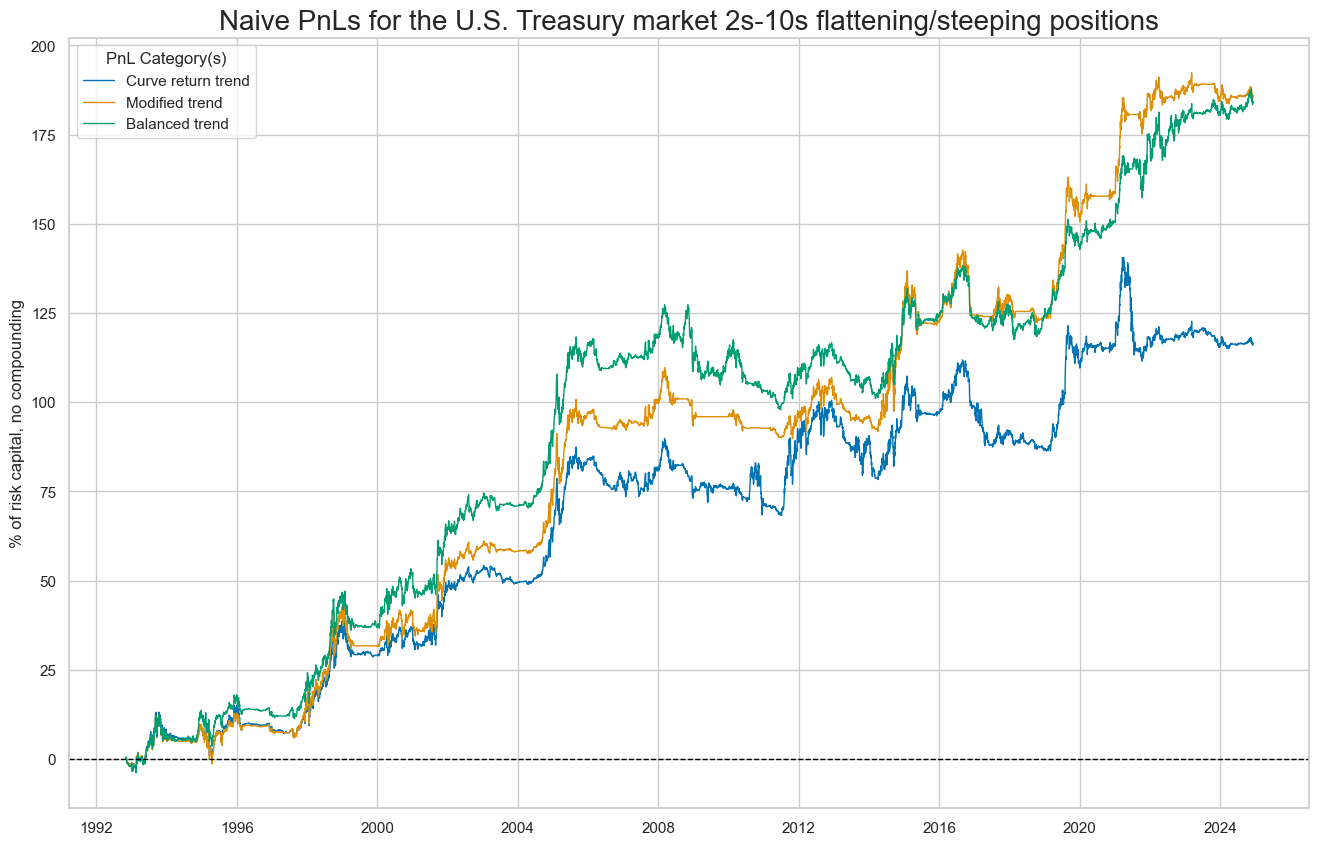
pnls = [sig + "_PZN0" for sig in sigx[:3]] # + ["Long only"]
naive_pnl.plot_pnls(
pnl_cats=pnls,
pnl_cids=["ALL"],
start=start,
title='Naive PnLs for the U.S. Treasury market 2s-10s flattening/steeping positions',
xcat_labels=['Curve return trend','Modified trend', 'Balanced trend'],
figsize=(16, 10),
)
dix = dict_crv
sigx = dix["sigs"]
start = dix["start"]
cidx = dix["cidx"]
naive_pnl = dix["pnls"]
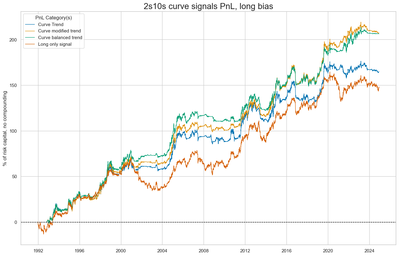
pnls = [sig + "_PZN1" for sig in sigx[:3]] + ["Long only"]
naive_pnl.plot_pnls(
pnl_cats=pnls,
pnl_cids=["ALL"],
start=start,
title='2s10s curve signals PnL, long bias',
xcat_labels=['Curve Trend','Curve modified trend', 'Curve balanced trend', 'Long only signal'],
figsize=(16, 10),
)
dix = dict_crv
sigx = dix["sigs"]
start = dix["start"]
cidx = dix["cidx"]
naive_pnl = dix["pnls"]
pnls = [s + "_PZN" + str(bias) for s in sigx for bias in [0, 1]] + ["Long only"]
df_eval = naive_pnl.evaluate_pnls(
pnl_cats=pnls,
pnl_cids=["ALL"],
start=start,
)
column_mapping = {
'ALL_CZS_ZN_NEG_PZN0': 'Macro trend',
'ALL_CZS_ZN_NEG_PZN1': 'Long macro trend',
'GB10v02YXR_BALTREND_ALL_PZN0': 'Curve balanced trend',
'GB10v02YXR_BALTREND_ALL_PZN1': 'Long curve balanced trend',
'GB10v02YXR_MODTREND_ALL_ZN_PZN0': 'Curve modified trend',
'GB10v02YXR_MODTREND_ALL_ZN_PZN1': 'Long curve modified trend',
'GB10v02YXR_TREND_ZN_PZN0': 'Pure trend',
'GB10v02YXR_TREND_ZN_PZN1': 'Long pure trend'
}
# Rename the columns
df_eval = df_eval.rename(columns=column_mapping)
display(df_eval.transpose())
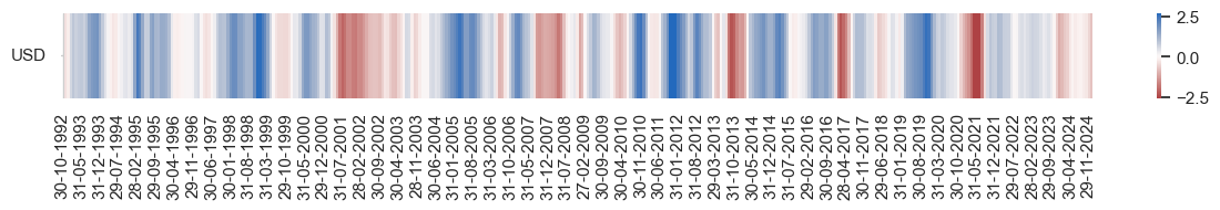
naive_pnl.signal_heatmap(
pnl_name=pnls[0],
freq="m",
title=None,
figsize=(15, 1)
)
| Return % | St. Dev. % | Sharpe Ratio | Sortino Ratio | Max 21-Day Draw % | Max 6-Month Draw % | Peak to Trough Draw % | Top 5% Monthly PnL Share | USD_GB10YXR_NSA correl | Traded Months | |
|---|---|---|---|---|---|---|---|---|---|---|
| xcat | ||||||||||
| Pure trend | 3.626716 | 10.0 | 0.362672 | 0.518862 | -16.317988 | -26.628695 | -28.980728 | 1.355031 | 0.282438 | 396 |
| Long pure trend | 5.135761 | 10.0 | 0.513576 | 0.736711 | -14.055082 | -20.133959 | -23.744033 | 0.958309 | 0.530577 | 396 |
| Curve modified trend | 5.787929 | 10.0 | 0.578793 | 0.841961 | -14.067912 | -18.367962 | -20.411058 | 0.943389 | 0.303118 | 396 |
| Long curve modified trend | 6.466872 | 10.0 | 0.646687 | 0.931766 | -16.323292 | -20.94325 | -22.490881 | 0.761008 | 0.535111 | 396 |
| Curve balanced trend | 5.734175 | 10.0 | 0.573417 | 0.830782 | -14.045807 | -20.165742 | -29.393009 | 0.775882 | 0.24853 | 396 |
| Long curve balanced trend | 6.429757 | 10.0 | 0.642976 | 0.928352 | -14.945659 | -19.079364 | -21.552015 | 0.703105 | 0.50875 | 396 |
| Macro trend | 6.062649 | 10.0 | 0.606265 | 0.882667 | -14.043297 | -29.296527 | -42.231735 | 0.723006 | 0.124206 | 396 |
| Long macro trend | 7.003965 | 10.0 | 0.700397 | 1.012699 | -13.664421 | -16.580417 | -18.883043 | 0.630917 | 0.411549 | 396 |
| Long only | 4.479399 | 10.0 | 0.44794 | 0.630097 | -13.64143 | -25.70485 | -36.261188 | 0.926593 | 0.620237 | 396 |
Annex: Pure economic directional signals #
Specs and panel tests #
sigs = [key + "_ZN" for key in dict_all.keys()] + ["ALL_CZS_ZN",]
labs= [val[1] for val in dict_all.values()]
targ = ["GB05YXR_NSA"]
cidx = cids_gb
start = "1992-01-01"

dict_ecodir = {
    "sigs": sigs,
    "targs": targ,
    "cidx": cidx,
    "labs": labs,
    "start": start,
    "srr": None,
    "pnls": None,
    "labs": labs
}
dix = dict_ecodir
sigs = dix["sigs"][:-1]
targ = dix["targs"][0]
cidx = dix["cidx"]
start = dix["start"]
# Initialize the dictionary to store CategoryRelations instances
dict_cr = {}
for sig in sigs:
dict_cr[sig] = msp.CategoryRelations(
dfx,
xcats=[sig, targ],
cids=cidx,
freq="M",
lag=1,
xcat_aggs=["last", "sum"],
start=start,
)
# Plotting the results
crs = list(dict_cr.values())
crs_keys = list(dict_cr.keys())
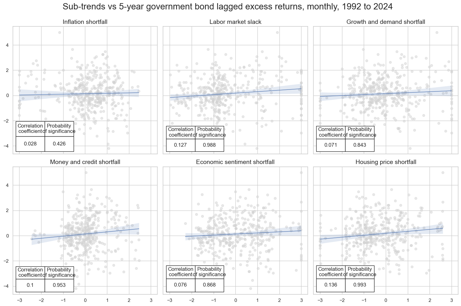
msv.multiple_reg_scatter(
cat_rels=crs,
title='Sub-trends vs 5-year government bond lagged excess returns, monthly, 1992 to 2024',
ylab=None,
ncol=3,
nrow=2,
# separator = 2008,
figsize=(15, 10),
prob_est="pool",
coef_box="lower left",
subplot_titles=labs
)
Accuracy and correlation check #
dix = dict_ecodir

sigx = dix["sigs"]
targx = [dix["targs"][0]]
cidx = dix["cidx"]
start = dix["start"]
labs = dix['labs'] + ['Macro']

srr = mss.SignalReturnRelations(
    dfx,
    cids=cidx,
    sigs=sigx,
    rets=targx,
    freqs="M",
    start=start,
)

dix["srr"] = srr
dix = dict_ecodir
srr = dix["srr"]

col_mapping = {
    'INFSHORT_ZN': "Inflation shortfall",
    'LABSLACK_ZN': "Labor market slack",
    'GRDSHORT_ZN': "Growth and demand shortfall",
    'MCRSHORT_ZN': "Money and credit shortfall",
    'SENTSHORT_ZN': "Economic sentiment shortfall",
    'HPISHORT_ZN': "Housing price shortfall",
    'ALL_CZS_ZN': "Macro"
}
srrx = srr.signals_table().reset_index()
srrx['Signal'] = srrx['Signal'].apply(lambda x: col_mapping.get(x, x))
srrx = srrx.set_index(['Return','Signal','Frequency','Aggregation'])
display(srrx.sort_index().astype("float").round(3))
| accuracy | bal_accuracy | pos_sigr | pos_retr | pos_prec | neg_prec | pearson | pearson_pval | kendall | kendall_pval | auc | ||||
|---|---|---|---|---|---|---|---|---|---|---|---|---|---|---|
| Return | Signal | Frequency | Aggregation | |||||||||||
| GB05YXR_NSA | Economic sentiment shortfall | M | last | 0.559 | 0.559 | 0.501 | 0.547 | 0.606 | 0.513 | 0.076 | 0.132 | 0.063 | 0.061 | 0.560 |
| Growth and demand shortfall | M | last | 0.532 | 0.544 | 0.387 | 0.547 | 0.601 | 0.488 | 0.071 | 0.157 | 0.035 | 0.301 | 0.543 | |
| Housing price shortfall | M | last | 0.519 | 0.531 | 0.390 | 0.547 | 0.584 | 0.477 | 0.136 | 0.007 | 0.087 | 0.010 | 0.530 | |
| Inflation shortfall | M | last | 0.506 | 0.497 | 0.600 | 0.547 | 0.544 | 0.449 | 0.028 | 0.574 | 0.014 | 0.680 | 0.497 | |
| Labor market slack | M | last | 0.539 | 0.572 | 0.289 | 0.547 | 0.649 | 0.495 | 0.127 | 0.012 | 0.099 | 0.003 | 0.560 | |
| Macro | M | last | 0.524 | 0.540 | 0.359 | 0.547 | 0.599 | 0.482 | 0.135 | 0.007 | 0.097 | 0.004 | 0.538 | |
| Money and credit shortfall | M | last | 0.544 | 0.544 | 0.501 | 0.547 | 0.591 | 0.497 | 0.100 | 0.047 | 0.104 | 0.002 | 0.545 |
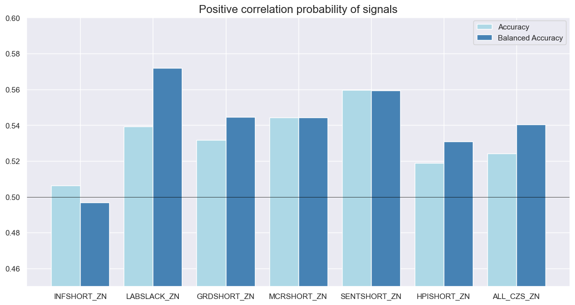
srr.accuracy_bars(
    type="signals",
    size=(14, 7),
    title="Positive correlation probability of signals",
)
Annex: Pure economic curve signals #
Specs and panel tests #
sigs= [key + "_ZN_NEG" for key in dict_all.keys()] + ["ALL_CZS_ZN_NEG",]

targ = ["GB10v2VTXR"]
cidx = cids_gb
start = "1992-01-01"
labs= [val[1] for val in dict_all.values()]

dict_ecocrv = {
    "sigs": sigs,
    "targs": targ,
    "cidx": cidx,
    "start": start,
    "srr": None,
    "pnls": None,
    "labs": labs
}
dix = dict_ecocrv
sigs = dix["sigs"][:-1]
targ = dix["targs"][0]
cidx = dix["cidx"]
start = dix["start"]
labs = dix['labs']
# Initialize the dictionary to store CategoryRelations instances
dict_cr = {}
for sig in sigs:
dict_cr[sig] = msp.CategoryRelations(
dfx,
xcats=[sig, targ],
cids=cidx,
freq="M",
lag=1,
xcat_aggs=["last", "sum"],
start=start,
)
# Plotting the results
crs = list(dict_cr.values())
crs_keys = list(dict_cr.keys())
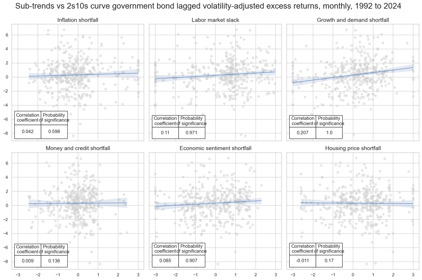
msv.multiple_reg_scatter(
cat_rels=crs,
title='Sub-trends vs 2s10s curve government bond lagged volatility-adjusted excess returns, monthly, 1992 to 2024',
ylab=None,
ncol=3,
nrow=2,
# separator = 2008,
figsize=(15, 10),
prob_est="pool",
coef_box="lower left",
subplot_titles=labs
)
Accuracy and correlation check #
dix = dict_ecocrv

sigx = dix["sigs"]
targx = [dix["targs"][0]]
cidx = dix["cidx"]
start = dix["start"]

srr = mss.SignalReturnRelations(
    dfx,
    cids=cidx,
    sigs=sigx,
    rets=targx,
    freqs="M",
    start=start,
)

dix["srr"] = srr
dix = dict_ecocrv
srr = dix["srr"]
display(srr.signals_table().sort_index().astype("float").round(3))
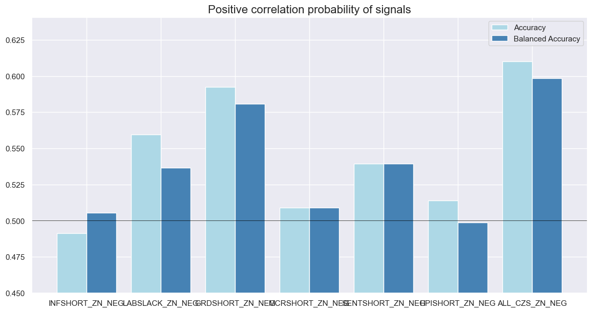
srr.accuracy_bars(
type="signals",
size=(14, 7),
title="Positive correlation probability of signals",
)
| accuracy | bal_accuracy | pos_sigr | pos_retr | pos_prec | neg_prec | pearson | pearson_pval | kendall | kendall_pval | auc | ||||
|---|---|---|---|---|---|---|---|---|---|---|---|---|---|---|
| Return | Signal | Frequency | Aggregation | |||||||||||
| GB10v2VTXR | ALL_CZS_ZN_NEG | M | last | 0.610 | 0.598 | 0.641 | 0.57 | 0.640 | 0.556 | 0.129 | 0.010 | 0.109 | 0.001 | 0.592 |
| GRDSHORT_ZN_NEG | M | last | 0.592 | 0.581 | 0.613 | 0.57 | 0.632 | 0.529 | 0.207 | 0.000 | 0.140 | 0.000 | 0.578 | |
| HPISHORT_ZN_NEG | M | last | 0.514 | 0.499 | 0.610 | 0.57 | 0.568 | 0.429 | -0.011 | 0.830 | 0.006 | 0.847 | 0.499 | |
| INFSHORT_ZN_NEG | M | last | 0.491 | 0.505 | 0.400 | 0.57 | 0.576 | 0.435 | 0.042 | 0.402 | 0.036 | 0.283 | 0.505 | |
| LABSLACK_ZN_NEG | M | last | 0.559 | 0.537 | 0.711 | 0.57 | 0.591 | 0.482 | 0.110 | 0.029 | 0.068 | 0.043 | 0.531 | |
| MCRSHORT_ZN_NEG | M | last | 0.509 | 0.509 | 0.499 | 0.57 | 0.579 | 0.439 | 0.009 | 0.864 | 0.034 | 0.319 | 0.509 | |
| SENTSHORT_ZN_NEG | M | last | 0.539 | 0.539 | 0.499 | 0.57 | 0.609 | 0.470 | 0.085 | 0.093 | 0.071 | 0.035 | 0.540 |
dix = dict_dir
srr = dix["srr"]
col_mapping = {
    'ALL_CZS_ZN': "Macro trend",
    'GB05YXR_BALTREND_ALL': "Balanced trend",
    'GB05YXR_MODTREND_ALL_ZN': "Modified trend",
    'GB05YXR_TREND_ZN': "Pure return trend",
}
srrx = srr.signals_table().reset_index()
srrx['Signal'] = srrx['Signal'].apply(lambda x: col_mapping.get(x, x))
srrx = srrx.set_index(['Return','Signal','Frequency','Aggregation'])
display(srrx.sort_index().astype("float").round(3))

srr.accuracy_bars(
    type="signals",
    size=(12, 7),
    title="Positive correlation probability of signals",
)
| accuracy | bal_accuracy | pos_sigr | pos_retr | pos_prec | neg_prec | pearson | pearson_pval | kendall | kendall_pval | auc | ||||
|---|---|---|---|---|---|---|---|---|---|---|---|---|---|---|
| Return | Signal | Frequency | Aggregation | |||||||||||
| GB05YXR_NSA | Balanced trend | M | last | 0.547 | 0.548 | 0.488 | 0.547 | 0.597 | 0.500 | 0.122 | 0.016 | 0.099 | 0.003 | 0.549 |
| Macro trend | M | last | 0.524 | 0.540 | 0.359 | 0.547 | 0.599 | 0.482 | 0.135 | 0.007 | 0.097 | 0.004 | 0.538 | |
| Modified trend | M | last | 0.552 | 0.547 | 0.565 | 0.547 | 0.588 | 0.506 | 0.096 | 0.058 | 0.084 | 0.013 | 0.547 | |
| Pure return trend | M | last | 0.552 | 0.547 | 0.565 | 0.547 | 0.588 | 0.506 | 0.056 | 0.267 | 0.054 | 0.109 | 0.547 |