Robust equity trends #
Get packages and JPMaQS data #
import numpy as np
import pandas as pd
from pandas import Timestamp
import matplotlib.pyplot as plt
import seaborn as sns
from scipy.stats import norm
import itertools

import warnings
import os
from datetime import date

import macrosynergy.management as msm
import macrosynergy.panel as msp
import macrosynergy.signal as mss
import macrosynergy.pnl as msn
import macrosynergy.visuals as msv
from macrosynergy.download import JPMaQSDownload
from macrosynergy.management.utils import merge_categories

warnings.simplefilter("ignore")
# Equity cross-section lists

cids_g3 = ["EUR", "JPY", "USD"]  # DM large
cids_dmxg3 = ["AUD", "CAD", "CHF", "GBP", "SEK"]  # DM small
cids_dmeq = sorted(cids_g3 + cids_dmxg3)
cids = cids_dmeq

cids_dm90 = ["GBP", "JPY", "USD"]  # countries with sufficient data for 1990s
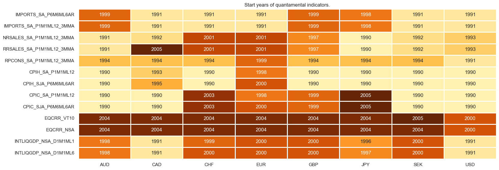
# Domestic spending growth
imports = ["IMPORTS_SA_P6M6ML6AR", "IMPORTS_SA_P1M1ML12_3MMA"]
rsales = [
"NRSALES_SA_P1M1ML12_3MMA",
"RRSALES_SA_P1M1ML12_3MMA",
"NRSALES_SA_P1Q1QL4",
"RRSALES_SA_P1Q1QL4",
]
pcons = ["RPCONS_SA_P1M1ML12_3MMA", "RPCONS_SA_P1Q1QL4"]
domspend = imports + rsales + pcons
# CPI inflation
cpi = [
"CPIH_SA_P1M1ML12",
"CPIH_SJA_P6M6ML6AR",
"CPIC_SA_P1M1ML12",
"CPIC_SJA_P6M6ML6AR",
]
liq = [
# liquidity intervention
"INTLIQGDP_NSA_D1M1ML1",
"INTLIQGDP_NSA_D1M1ML6",
]
# Real equity index carry
rcry = ["EQCRR_VT10", "EQCRR_NSA"]
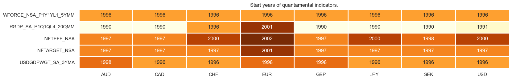
# Supporting economic indicators
wforce = ["WFORCE_NSA_P1Y1YL1_5YMM"]
nomgdp = ["RGDP_SA_P1Q1QL4_20QMM", "INFTEFF_NSA", "INFTARGET_NSA", "USDGDPWGT_SA_3YMA"]
# Market indicators
markets = ["EQXR_NSA"]
# Composite lists
mains = domspend + cpi + rcry + liq
supports = wforce + nomgdp
xcats = mains + supports + markets
# Resultant tickers
tickers = [cid + "_" + xcat for cid in cids for xcat in xcats]
print(f"Maximum number of tickers is {len(tickers)}")
Maximum number of tickers is 176
client_id: str = os.getenv("DQ_CLIENT_ID")
client_secret: str = os.getenv("DQ_CLIENT_SECRET")

with JPMaQSDownload(oauth=True, client_id=client_id, client_secret=client_secret) as dq:
    assert dq.check_connection()
    df = dq.download(
        tickers=tickers,
        start_date="1990-01-01",
        suppress_warning=True,
        metrics=["value"],
        show_progress=True,
    )
    assert isinstance(df, pd.DataFrame) and not df.empty

print("Last updated:", date.today())
Downloading data from JPMaQS.
Timestamp UTC:  2025-11-06 13:03:58
Connection successful!
Requesting data: 100%|██████████| 9/9 [00:01<00:00,  4.93it/s]
Downloading data: 100%|██████████| 9/9 [01:40<00:00, 11.15s/it]
Some expressions are missing from the downloaded data. Check logger output for complete list.
24 out of 176 expressions are missing. To download the catalogue of all available expressions and filter the unavailable expressions, set `get_catalogue=True` in the call to `JPMaQSDownload.download()`.
Last updated: 2025-11-06
dfx = df.copy().sort_values(["cid", "xcat", "real_date"])
dfx.info()
<class 'pandas.core.frame.DataFrame'>
Index: 1169964 entries, 99382 to 1136353
Data columns (total 4 columns):
 #   Column     Non-Null Count    Dtype
---  ------     --------------    -----
 0   real_date  1169964 non-null  datetime64[ns]
 1   cid        1169964 non-null  object
 2   xcat       1169964 non-null  object
 3   value      1169964 non-null  float64
dtypes: datetime64[ns](1), float64(1), object(2)
memory usage: 44.6+ MB
Rename quarterly tickers to roughly equivalent monthly tickers to simplify subsequent operations.
Renaming and availability check #
Renaming #
dict_repl = {
    # Labour
    "RPCONS_SA_P1Q1QL4": "RPCONS_SA_P1M1ML12_3MMA",
    "RRSALES_SA_P1Q1QL4": "RRSALES_SA_P1M1ML12_3MMA",
    "NRSALES_SA_P1Q1QL4": "NRSALES_SA_P1M1ML12_3MMA",
}

# Ensure 'xcat' exists in dfx before replacement
if "xcat" in dfx.columns:
    dfx["xcat"] = dfx["xcat"].replace(dict_repl, regex=False)
else:
    print("Column 'xcat' not found in dfx.")
Availability check #
xcatx = [xc for xc in mains if xc not in dict_repl.keys()]
msm.check_availability(dfx, xcats=xcatx, cids=cids_dmeq, missing_recent=False)
xcatx = [xc for xc in supports if xc not in dict_repl.keys()]
msm.check_availability(dfx, xcats=xcatx, cids=cids_dmeq, missing_recent=False)
msm.check_availability(dfx, xcats=markets, cids=cids, missing_recent=False)

Feature engineering and checks #
Domestic spending growth #
Transformations #
# Backward-extension of INFTARGET_NSA

# Duplicate targets
cidx = cids_dmeq
calcs = [f"INFTARGET_BX = INFTARGET_NSA"]
dfa = msp.panel_calculator(dfx, calcs, cids=cidx)

# Add all dates back to 1990 to the frame, filling "value " with NaN
all_dates = np.sort(dfx['real_date'].unique())
all_combinations = pd.DataFrame(
    list(itertools.product(dfa['cid'].unique(), dfa['xcat'].unique(), all_dates)),
    columns=['cid', 'xcat', 'real_date']
)
dfax = pd.merge(all_combinations, dfa, on=['cid', 'xcat', 'real_date'], how='left')

# Backfill the values with first target value
dfax = dfax.sort_values(by=['cid', 'xcat', 'real_date'])
dfax['value'] = dfax.groupby(['cid', 'xcat'])['value'].bfill()

dfx = msm.update_df(dfx, dfax)
# Extended effective inflation target by hierarchical merging

hierarchy = ["INFTEFF_NSA", "INFTARGET_BX"]
dfa = merge_categories(dfx, xcats=hierarchy, new_xcat="INFTEFF_BX")
dfx = msm.update_df(dfx, dfa)
# Excess growth

xcatx_nominal = [
    "IMPORTS_SA_P6M6ML6AR",
    "IMPORTS_SA_P1M1ML12_3MMA",
    "NRSALES_SA_P1M1ML12_3MMA",
]
xcatx_real = ["RRSALES_SA_P1M1ML12_3MMA", "RPCONS_SA_P1M1ML12_3MMA"]

calcs = [f"X{xc} = {xc} - RGDP_SA_P1Q1QL4_20QMM - INFTEFF_BX" for xc in xcatx_nominal]
calcs += [f"X{xc} = {xc} - RGDP_SA_P1Q1QL4_20QMM" for xc in xcatx_real]

dfa = msp.panel_calculator(
    dfx,
    calcs=calcs,
    cids=cids,
)
dfx = msm.update_df(dfx, dfa)
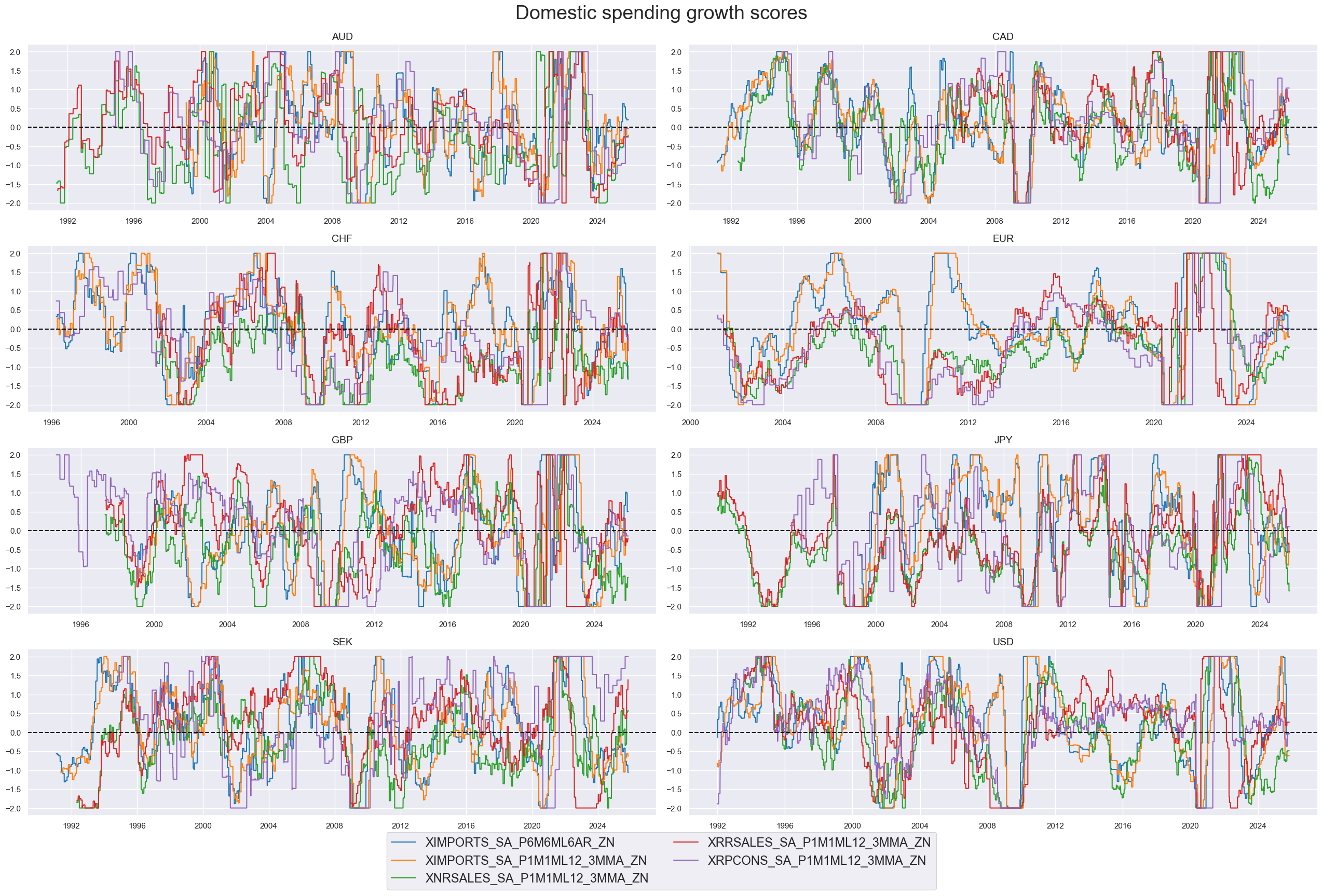
Structuring and scoring #
# Un-scored indicators and weights

dict_domspend = {
    "XIMPORTS_SA_P6M6ML6AR": 0.5,
    "XIMPORTS_SA_P1M1ML12_3MMA": 0.5,
    "XNRSALES_SA_P1M1ML12_3MMA": 0.5,
    "XRRSALES_SA_P1M1ML12_3MMA": 0.5,
    "XRPCONS_SA_P1M1ML12_3MMA": 1,
}
# Normalization of excess spending growth indicators

cidx = cids_dmeq
xcatx = list(dict_domspend.keys())
sdate = "1990-01-01"

for xc in xcatx:
    dfaa = msp.make_zn_scores(
        dfx,
        xcat=xc,
        cids=cidx,
        sequential=True,
        min_obs=261 * 5,
        neutral="zero",
        pan_weight=0.5,  # variance estimated based on panel and cross-sectional variation
        thresh=2,
        postfix="_ZN",
        est_freq="m",
    )
    dfa = msm.update_df(dfa, dfaa)

dfx = msm.update_df(dfx, dfa)
xspendz = [k + "_ZN" for k in list(dict_domspend.keys())]
xcatx = xspendz
cidx = cids
sdate = "1990-01-01"

msp.view_timelines(
    dfx,
    xcats=xcatx,
    cids=cidx,
    ncol=2,
    aspect=3,
    cumsum=False,
    start=sdate,
    same_y=False,
    all_xticks=True,
    legend_fontsize=17,
    title="Domestic spending growth scores",
    title_fontsize=27,
)
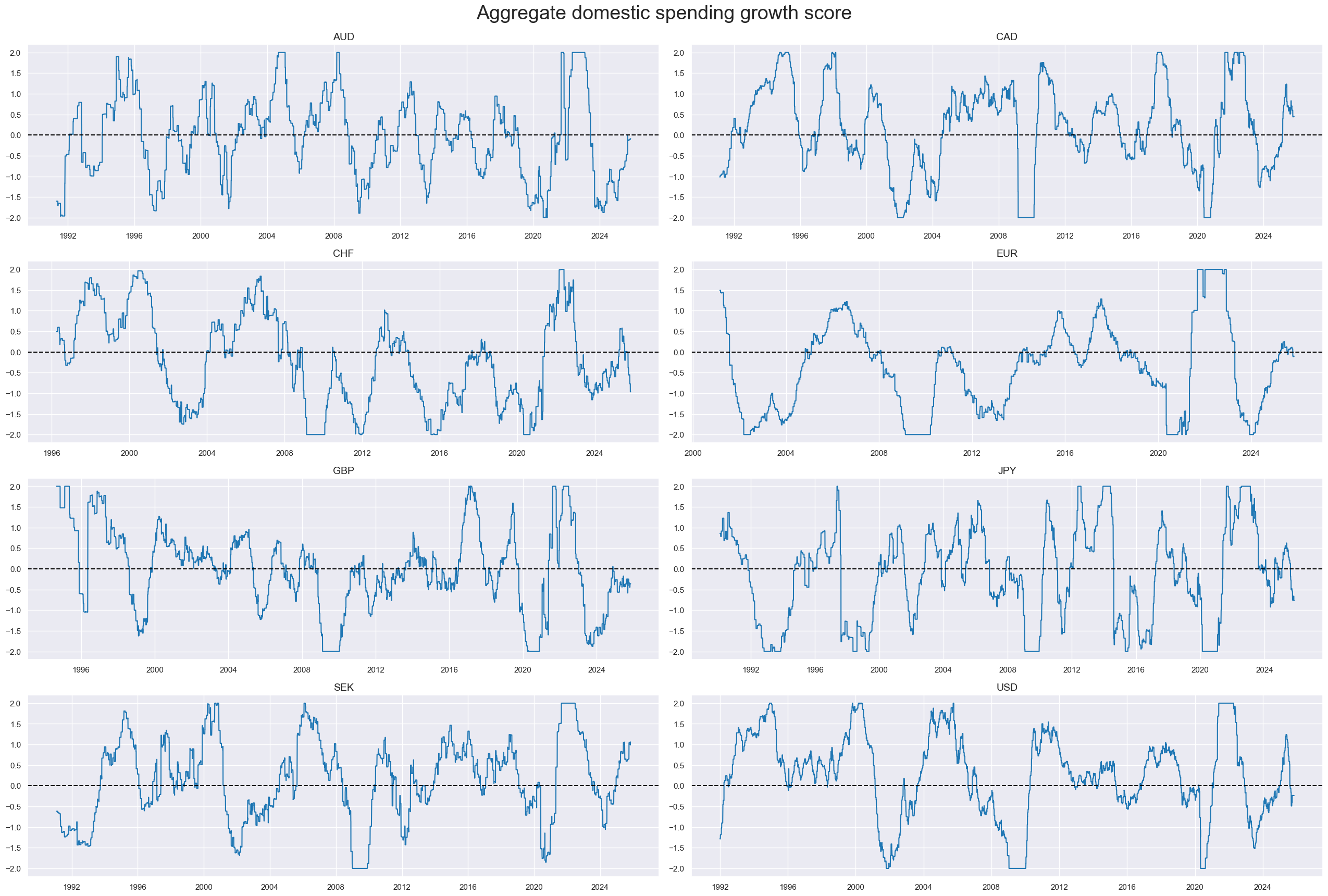
# Weighted linear combination

cidx = cids_dmeq
xcatx = xspendz
weights = list(dict_domspend.values())
czs = "XSPEND"

dfa = msp.linear_composite(
    dfx,
    xcats=xcatx,
    cids=cidx,
    weights=weights,
    normalize_weights=True,
    complete_xcats=False,
    new_xcat=czs,
)
dfx = msm.update_df(dfx, dfa)

# Re-scoring

dfa = msp.make_zn_scores(
    dfx,
    xcat=czs,
    cids=cidx,
    sequential=True,
    min_obs=261 * 5,
    neutral="zero",
    pan_weight=1,
    thresh=2,
    postfix="_ZN",
    est_freq="m",
)
dfx = msm.update_df(dfx, dfa)
xcatx = "XSPEND_ZN"
cidx = cids
sdate = "1990-01-01"

msp.view_timelines(
    dfx,
    xcats=xcatx,
    cids=cidx,
    ncol=2,
    aspect=3,
    cumsum=False,
    start=sdate,
    same_y=False,
    all_xticks=True,
    legend_fontsize=17,
    title="Aggregate domestic spending growth score",
    title_fontsize=27,
)
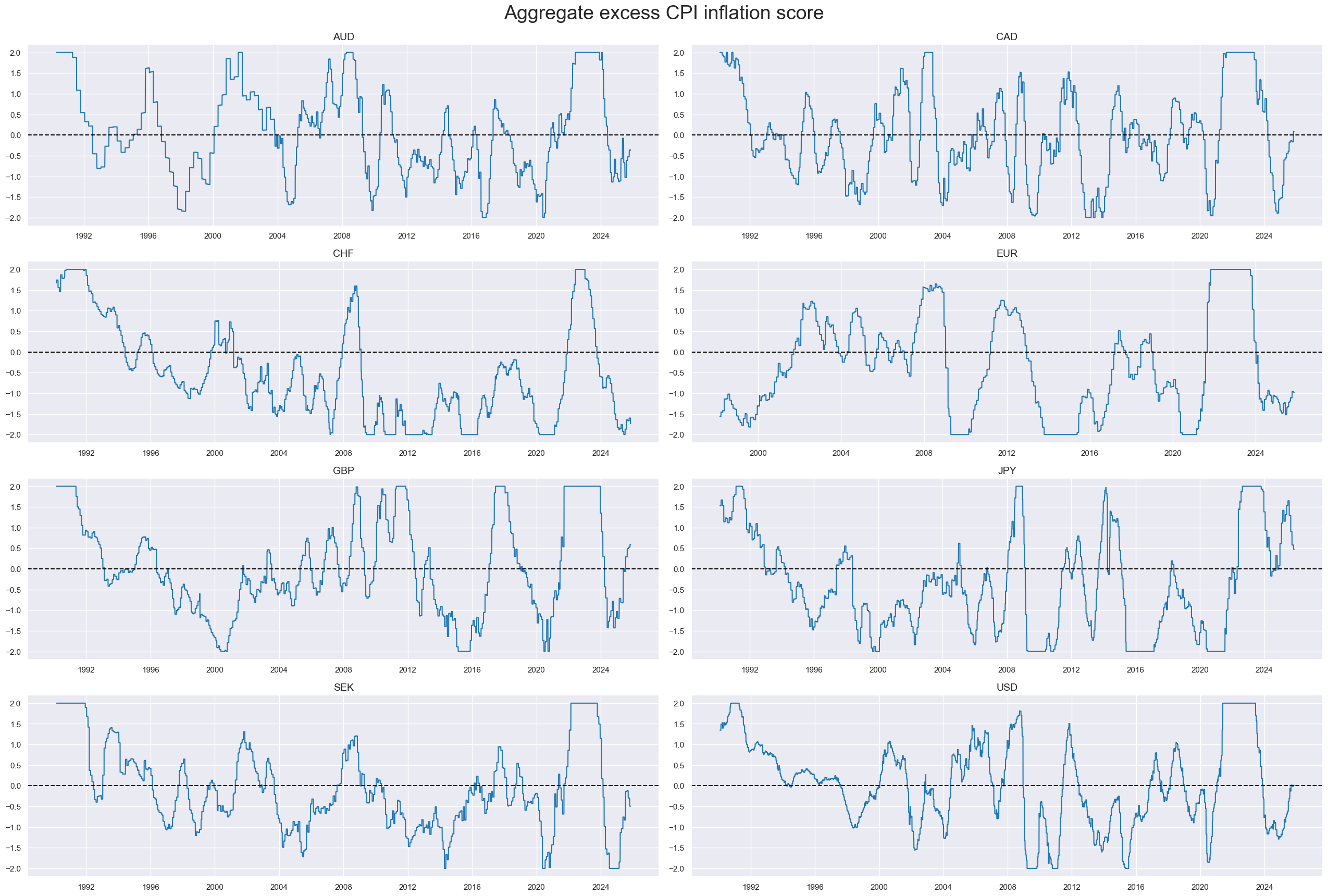
CPI inflation #
Transformations #
xcatx = cpi
calcs = [f"X{xc} = {xc} - INFTEFF_BX" for xc in xcatx]

dfa = msp.panel_calculator(
    dfx,
    calcs=calcs,
    cids=cids,
)
dfx = msm.update_df(dfx, dfa)
xinfs = list(dfa['xcat'].unique())
Structuring and scoring #
# Normalization of inflation indicators

cidx = cids_dmeq
xcatx = xinfs
sdate = "1990-01-01"

for xc in xcatx:
    dfaa = msp.make_zn_scores(
        dfx,
        xcat=xc,
        cids=cidx,
        sequential=True,
        min_obs=261 * 5,
        neutral="zero",
        pan_weight=0.5,  # variance estimated based on panel and cross-sectional variation
        thresh=2,
        postfix="_ZN",
        est_freq="m",
    )
    dfa = msm.update_df(dfa, dfaa)

dfx = msm.update_df(dfx, dfa)
xinfz = [xc + "_ZN" for xc in xinfs]
xcatx = xinfz
cidx = cids
sdate = "1990-01-01"

msp.view_timelines(
    dfx,
    xcats=xcatx,
    cids=cidx,
    ncol=2,
    aspect=3,
    cumsum=False,
    start=sdate,
    same_y=False,
    all_xticks=True,
    legend_fontsize=17,
    title="Excess CPI inflation scores",
    title_fontsize=27,
)

# Weighted linear combination

cidx = cids_dmeq
xcatx = xinfz
czs = "XINF"

dfa = msp.linear_composite(
    dfx,
    xcats=xcatx,
    cids=cidx,
    complete_xcats=False,
    new_xcat=czs,
)
dfx = msm.update_df(dfx, dfa)

# Re-scoring

dfa = msp.make_zn_scores(
    dfx,
    xcat=czs,
    cids=cidx,
    sequential=True,
    min_obs=261 * 5,
    neutral="zero",
    pan_weight=1,
    thresh=2,
    postfix="_ZN",
    est_freq="m",
)
dfx = msm.update_df(dfx, dfa)
xcatx = "XINF_ZN"
cidx = cids
sdate = "1990-01-01"

msp.view_timelines(
    dfx,
    xcats=xcatx,
    cids=cidx,
    ncol=2,
    aspect=3,
    cumsum=False,
    start=sdate,
    same_y=False,
    all_xticks=True,
    legend_fontsize=17,
    title="Aggregate excess CPI inflation score",
    title_fontsize=27,
)
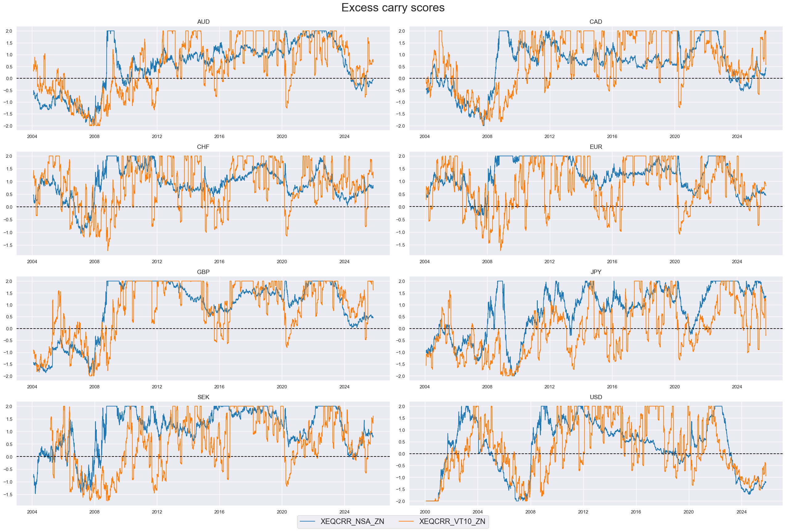
Equity carry #
Transformations #
# Excess real carry based on minimum carry Sharpe of approximately 0.3

calcs = [
    "XEQCRR_NSA = EQCRR_NSA - 4",
    "XEQCRR_VT10 = EQCRR_VT10 - 3",
]
dfa = msp.panel_calculator(
    dfx,
    calcs=calcs,
    cids=cids,
)
dfx = msm.update_df(dfx, dfa)

xcrs = dfa["xcat"].unique().tolist()
Structuring and scoring #
# Normalization of excess spending growth indicators

cidx = cids_dmeq
xcatx = xcrs
sdate = "1990-01-01"

for xc in xcatx:
    dfaa = msp.make_zn_scores(
        dfx,
        xcat=xc,
        cids=cidx,
        sequential=True,
        min_obs=261 * 5,
        neutral="zero",
        pan_weight=0.5,  # variance estimated based on panel and cross-sectional variation
        thresh=2,
        postfix="_ZN",
        est_freq="m",
    )
    dfa = msm.update_df(dfa, dfaa)

dfx = msm.update_df(dfx, dfa)
xcrz = [xc + "_ZN" for xc in xcrs]
xcatx = xcrz
cidx = cids
sdate = "1990-01-01"

msp.view_timelines(
    dfx,
    xcats=xcatx,
    cids=cidx,
    ncol=2,
    aspect=3,
    cumsum=False,
    start=sdate,
    same_y=False,
    all_xticks=True,
    legend_fontsize=17,
    title="Excess carry scores",
    title_fontsize=27,
)
# Weighted linear combination

cidx = cids_dmeq
xcatx = xcrz
czs = "XCRR"

dfa = msp.linear_composite(
    dfx,
    xcats=xcatx,
    cids=cidx,
    complete_xcats=False,
    new_xcat=czs,
)
dfx = msm.update_df(dfx, dfa)

# Re-scoring

dfa = msp.make_zn_scores(
    dfx,
    xcat=czs,
    cids=cidx,
    sequential=True,
    min_obs=261 * 5,
    neutral="zero",
    pan_weight=1,
    thresh=2,
    postfix="_ZN",
    est_freq="m",
)
dfx = msm.update_df(dfx, dfa)
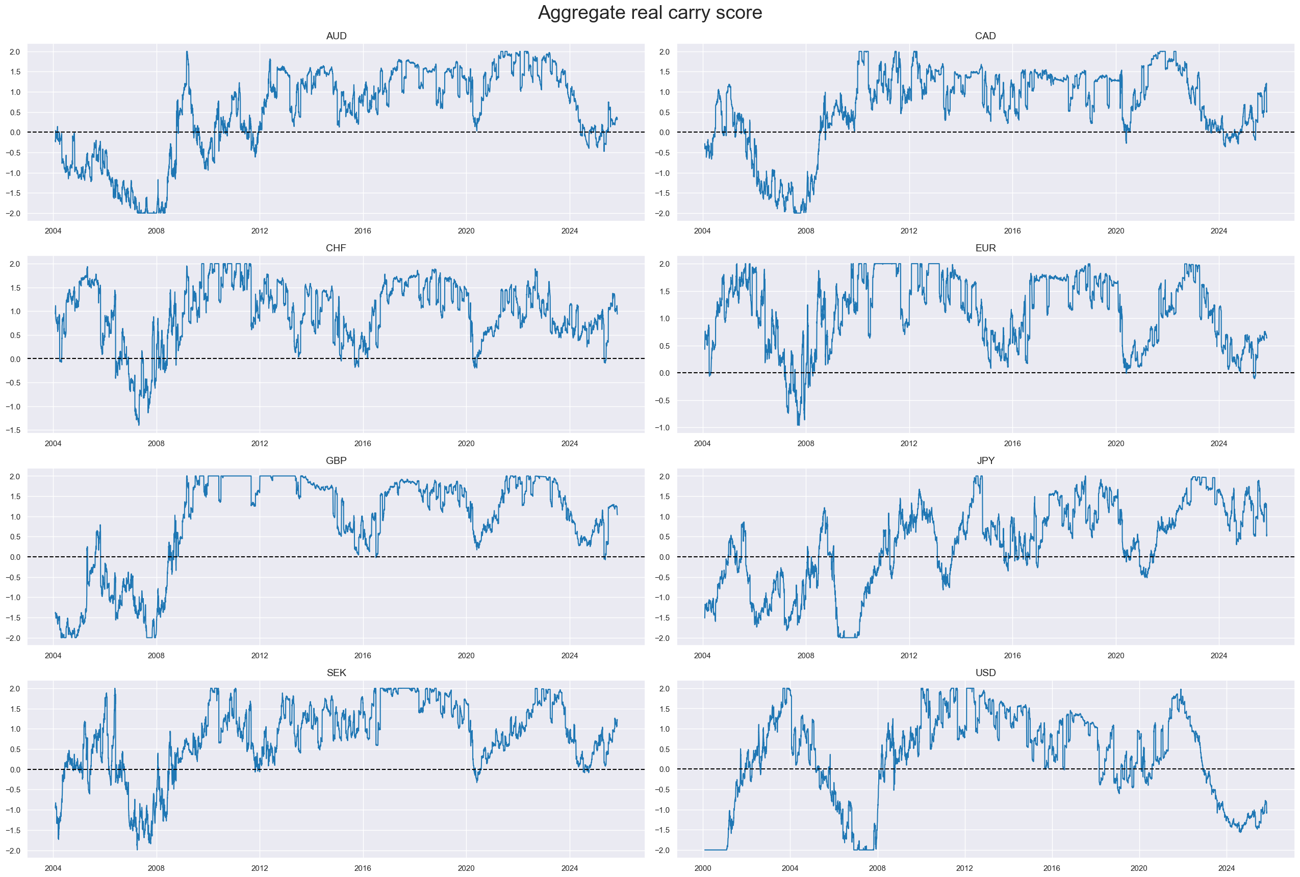
xcatx = "XCRR_ZN"
cidx = cids
sdate = "1990-01-01"

msp.view_timelines(
    dfx,
    xcats=xcatx,
    cids=cidx,
    ncol=2,
    aspect=3,
    cumsum=False,
    start=sdate,
    same_y=False,
    all_xticks=True,
    legend_fontsize=17,
    title="Aggregate real carry score",
    title_fontsize=27,
)
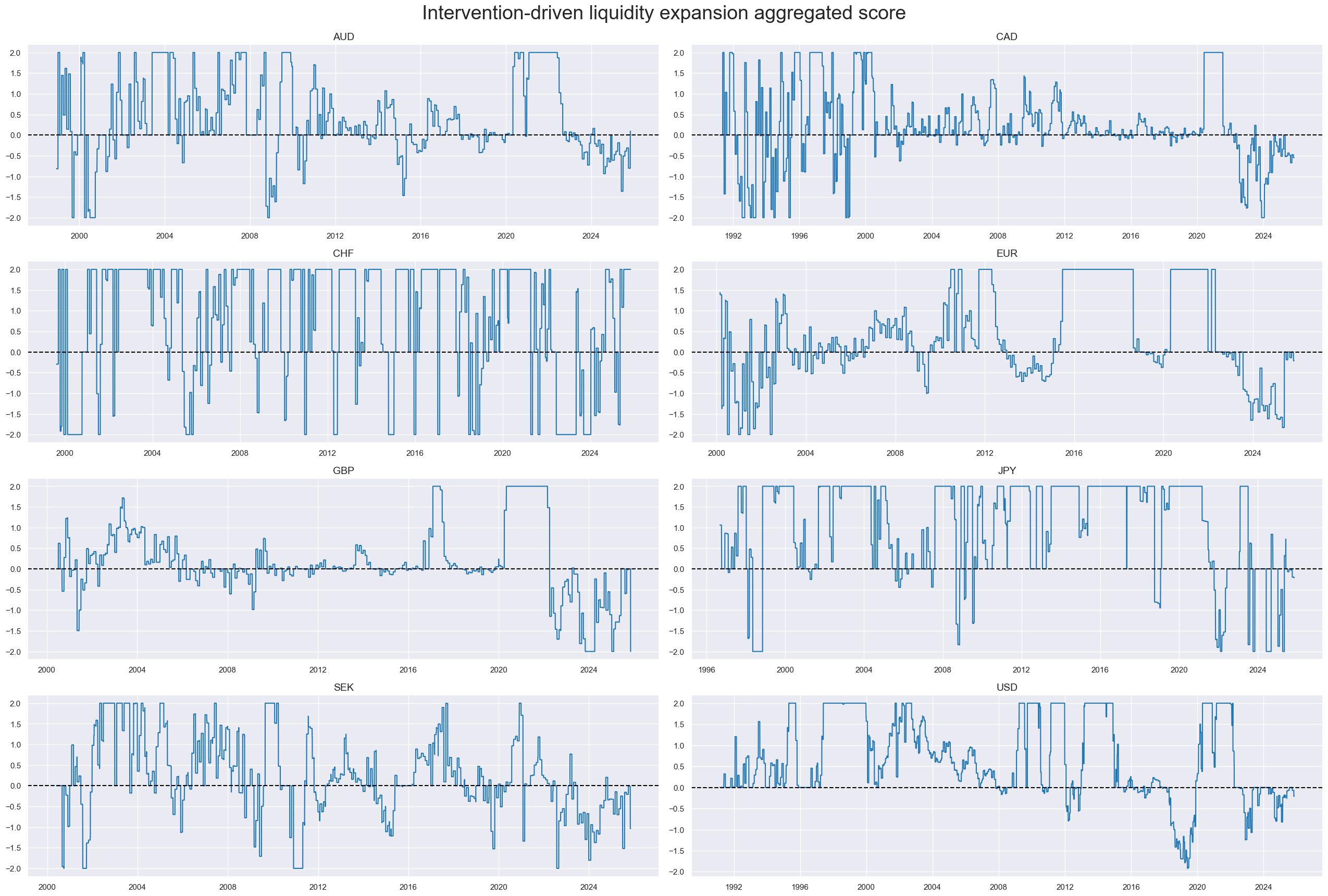
Intervention-driven liquidity expansion #
Structuring and scoring #
# Normalization of liquidity intervention indicators

cidx = cids_dmeq
xcatx = liq
sdate = "1990-01-01"

for xc in xcatx:
    dfaa = msp.make_zn_scores(
        dfx,
        xcat=xc,
        cids=cidx,
        sequential=True,
        min_obs=261 * 5,
        neutral="zero",
        pan_weight=0.5,  # variance estimated based on panel and cross-sectional variation
        thresh=2,
        postfix="_ZN",
        est_freq="m",
    )
    dfa = msm.update_df(dfa, dfaa)

dfx = msm.update_df(dfx, dfa)
xinfz = [xc + "_ZN" for xc in xinfs]
xcatx = liq
cidx = cids_dmeq
sdate = "1990-01-01"

msp.view_timelines(
    dfx,
    xcats=xcatx,
    cids=cidx,
    ncol=2,
    aspect=3,
    cumsum=False,
    start=sdate,
    same_y=False,
    all_xticks=True,
    legend_fontsize=17,
    title="Intervention-driven liquidity expansion, as % pf GDP ",
    title_fontsize=27,
)

# Weighted linear combination

cidx = cids_dmeq
xcatx = liq
czs = "LIQINT"

dfa = msp.linear_composite(
    dfx,
    xcats=xcatx,
    cids=cidx,
    complete_xcats=False,
    new_xcat=czs,
)
dfx = msm.update_df(dfx, dfa)

# Re-scoring

dfa = msp.make_zn_scores(
    dfx,
    xcat=czs,
    cids=cidx,
    sequential=True,
    min_obs=261 * 5,
    neutral="zero",
    pan_weight=1,
    thresh=2,
    postfix="_ZN",
    est_freq="m",
)
dfx = msm.update_df(dfx, dfa)
xcatx = "LIQINT_ZN"
cidx = cids
sdate = "1990-01-01"

msp.view_timelines(
    dfx,
    xcats=xcatx,
    cids=cidx,
    ncol=2,
    aspect=3,
    cumsum=False,
    start=sdate,
    same_y=False,
    all_xticks=True,
    legend_fontsize=17,
    title="Intervention-driven liquidity expansion aggregated score",
    title_fontsize=27,
)
Cross-category scores #
Thematic factor scores #
# Initiate dictionary for factor names

dict_names = {}
# Thematic support factors
xcatx_negs = ["XSPEND_ZN", "XINF_ZN"]
calcs = [f"{xc}_NEG = - {xc} " for xc in xcatx_negs]
dfa = msp.panel_calculator(
dfx,
calcs=calcs,
cids=cids,
)
dfx = msm.update_df(dfx, dfa)
factorz_xcr = dfa["xcat"].unique().tolist() + ["LIQINT_ZN"]
factorz = factorz_xcr + ["XCRR_ZN"]
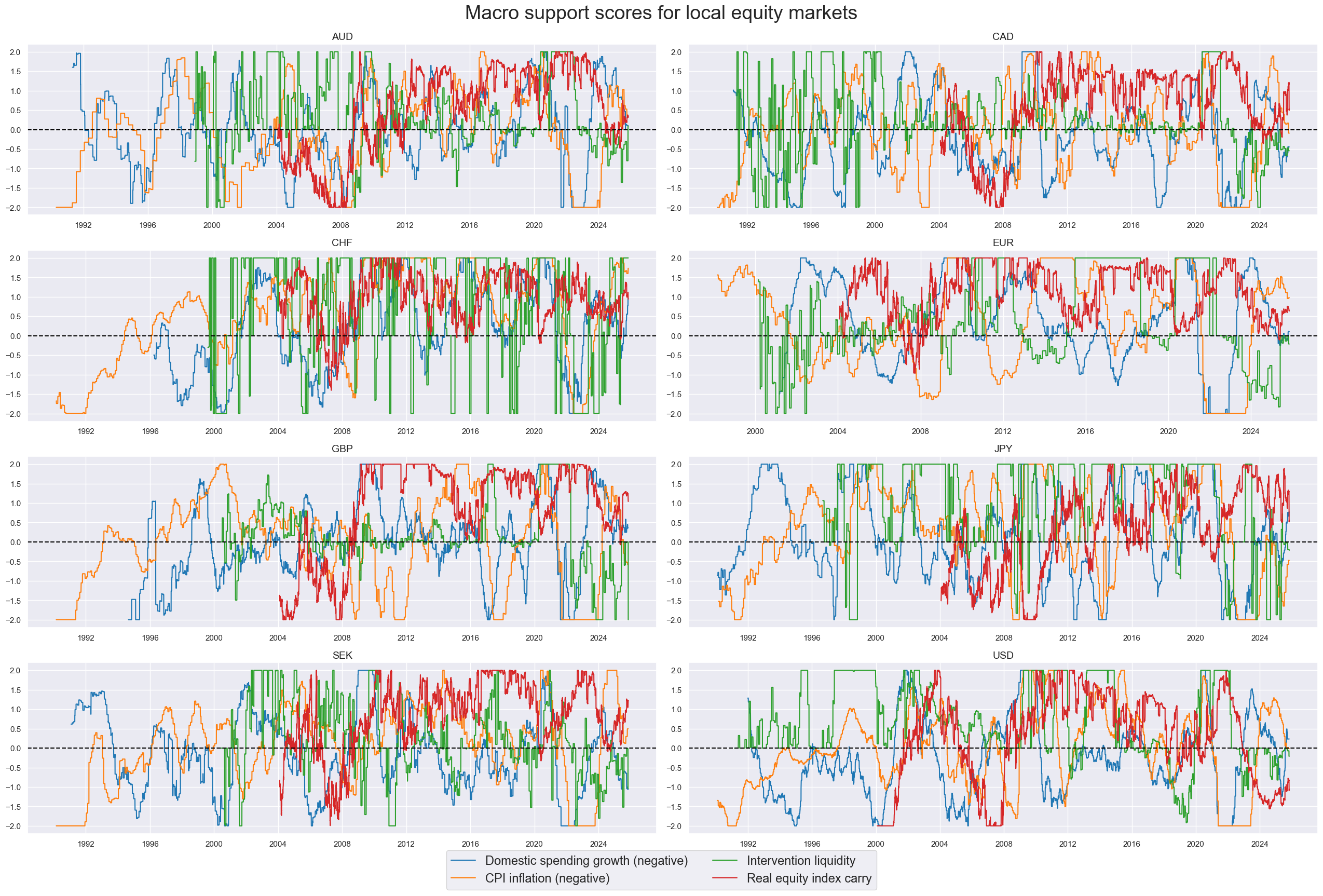
dict_names["XSPEND_ZN_NEG"] = "Domestic spending growth (negative)"
dict_names["XINF_ZN_NEG"] = "CPI inflation (negative)"
dict_names["XCRR_ZN"] = "Real equity index carry"
dict_names["LIQINT_ZN"] = "Intervention liquidity"
xcatx = factorz
cidx = cids
sdate = "1990-01-01"

msp.view_timelines(
    dfx,
    xcats=xcatx,
    cids=cidx,
    ncol=2,
    aspect=3,
    cumsum=False,
    start=sdate,
    same_y=False,
    all_xticks=True,
    legend_fontsize=17,
    title="Macro support scores for local equity markets",
    title_fontsize=27,
    xcat_labels=dict_names,
)
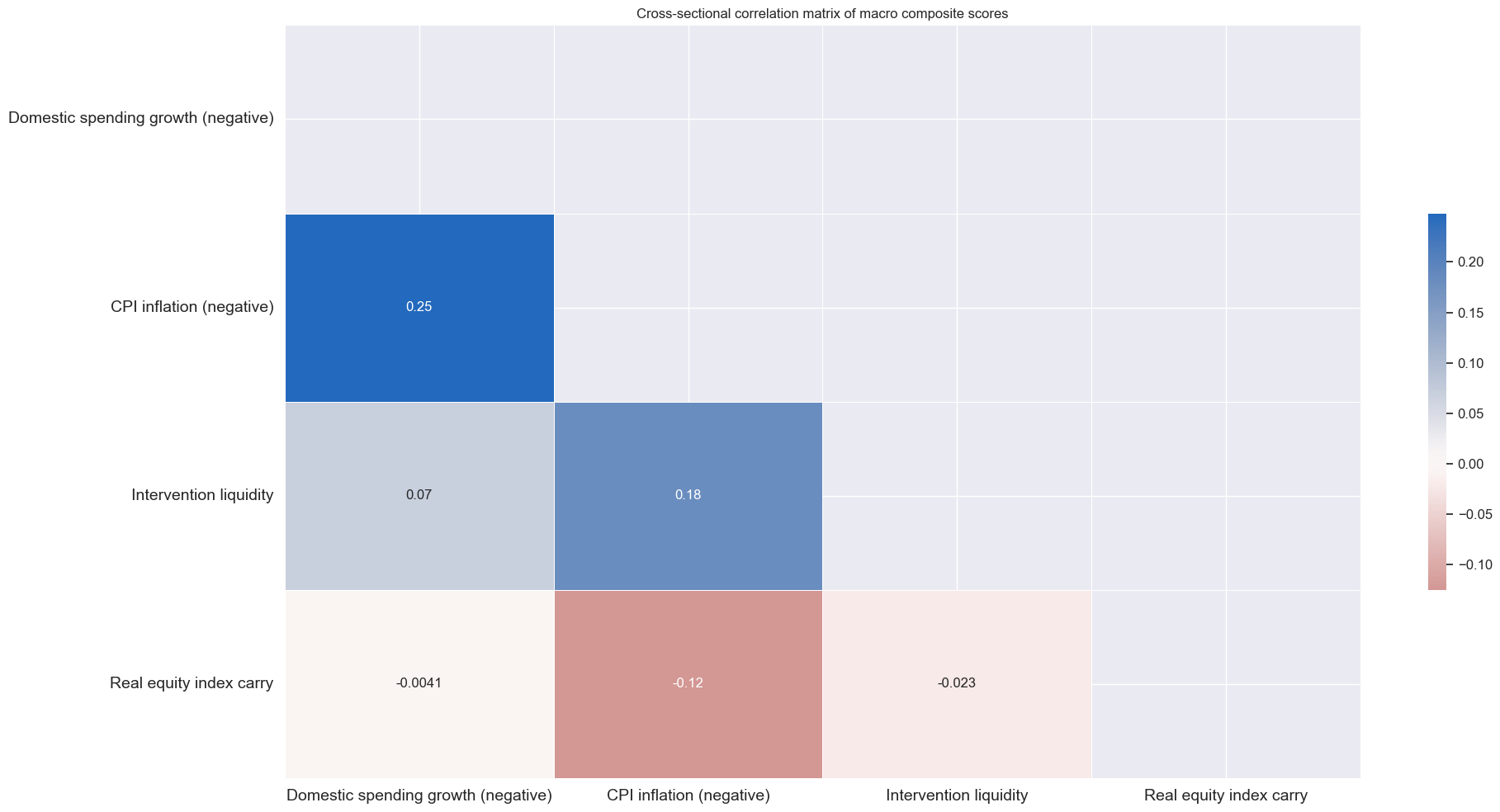
xcatx = factorz
cidx = cids_dmeq

msp.correl_matrix(
    dfx,
    xcats=xcatx,
    xcat_labels=[dict_names[xc] for xc in xcatx],
    cids=cidx,
    freq="M",
    title="Cross-sectional correlation matrix of macro composite scores",
    size=(20, 10),
    show=True,
    annot=True
)
Aggregate macro support scores #
# Weighted linear combinations
dict_macro = {
"MACRO": (factorz, cids_dmeq, "2004-01-01"),
"MACROX": (factorz_xcr, cids_dmeq, "2004-01-01"),
"MACROX90": (factorz_xcr, cids_dm90, "1990-01-01"),
}
for k, v in dict_macro.items():
xcatx = v[0]
cidx = v[1]
sdate = v[2]
dfa = msp.linear_composite(
dfx,
xcats=xcatx,
cids=cidx,
complete_xcats=False,
start=sdate,
new_xcat=k,
)
dfx = msm.update_df(dfx, dfa)
dfa = msp.make_zn_scores(
dfx,
xcat=k,
cids=cidx,
sequential=True,
min_obs=261 * 5,
neutral="zero",
pan_weight=1,
thresh=2,
postfix="_ZN",
est_freq="m",
)
dfx = msm.update_df(dfx, dfa)
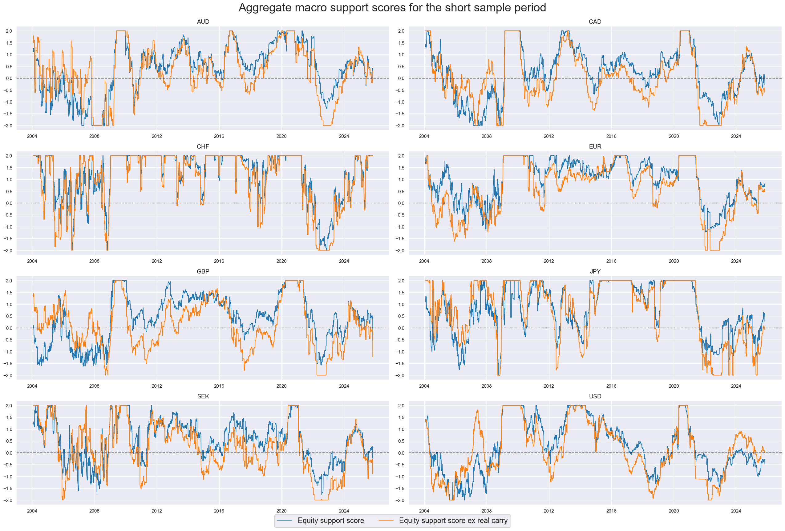
dict_names["MACRO_ZN"] = "Equity support score"
dict_names["MACROX_ZN"] = "Equity support score ex real carry"
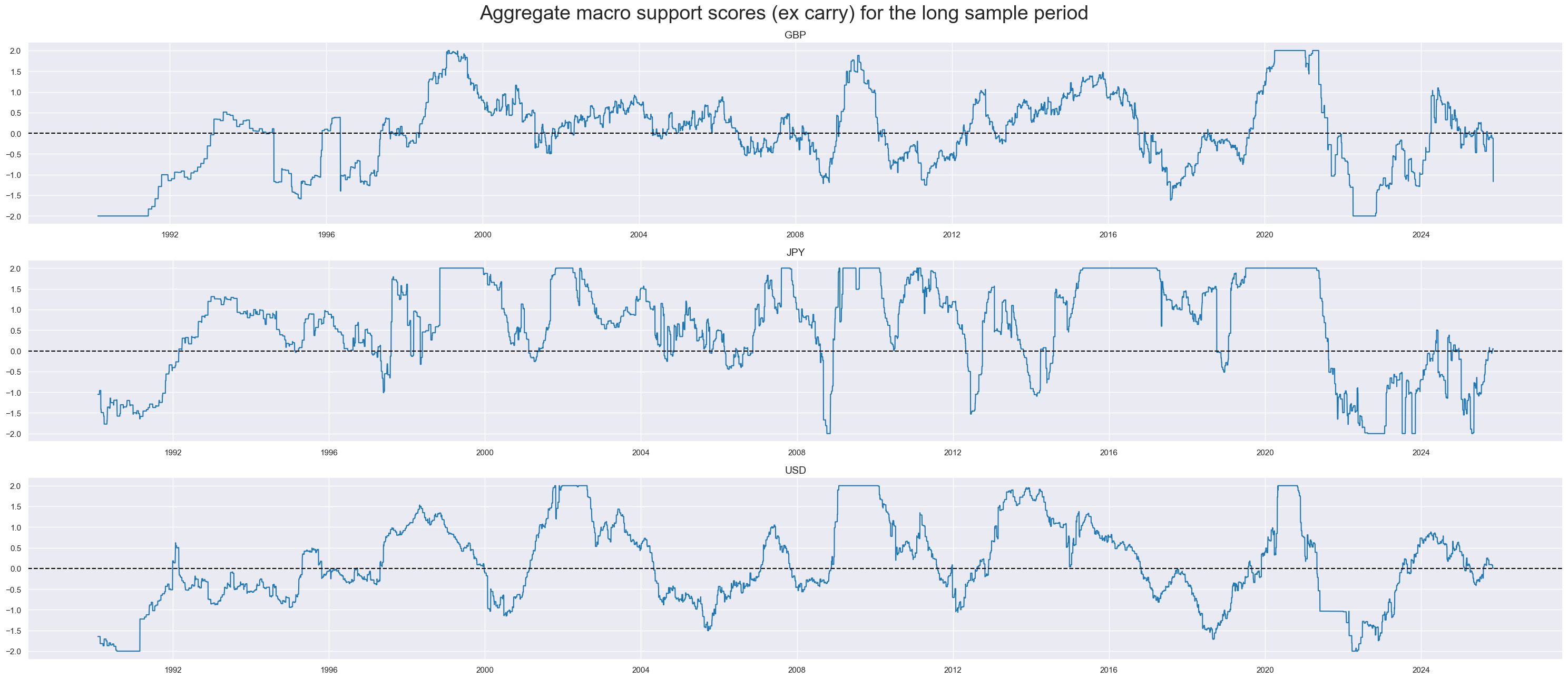
dict_names["MACROX90_ZN"] = "Equity support score ex real carry"
xcatx = ["MACRO_ZN", "MACROX_ZN"]
cidx = cids_dmeq

msp.view_timelines(
    dfx,
    xcats=xcatx,
    cids=cidx,
    ncol=2,
    aspect=3,
    cumsum=False,
    same_y=False,
    all_xticks=True,
    legend_fontsize=17,
    title="Aggregate macro support scores for the short sample period",
    title_fontsize=27,
    xcat_labels=dict_names,
)
xcatx = ["MACROX90_ZN"]
cidx = cids_dm90
sdate = "1990-01-01"

msp.view_timelines(
    dfx,
    xcats=xcatx,
    cids=cidx,
    ncol=1,
    aspect=7,
    all_xticks=True,
    legend_fontsize=17,
    title="Aggregate macro support scores (ex carry) for the long sample period",
    title_fontsize=27,
    start=sdate,
)
Robust equity returns trends and modification #
Robust trend #
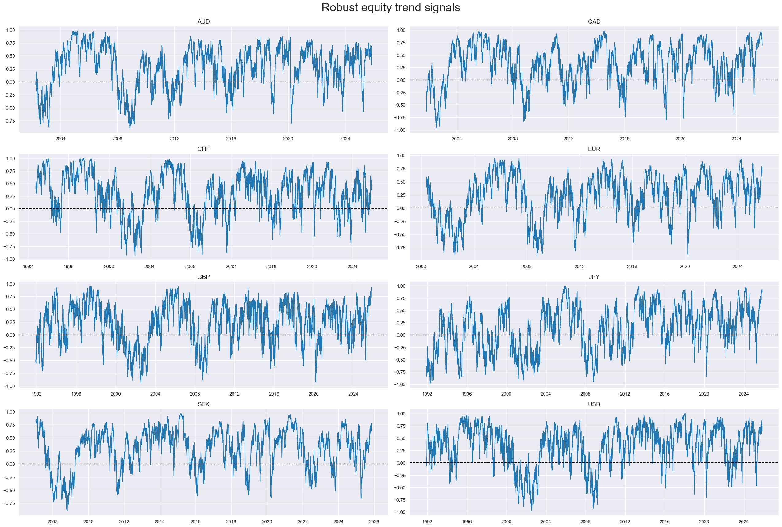
We use a trend-following signal following Tzotchev, D. (2018) , allowing us to test the macro-enhanced strategy using a different trend-following approach
# Creating a function that returns the cdf as dataframe
def norm_cdf_df(df):
    """Apply scipy.stats.norm.cdf to a DataFrame and return a DataFrame."""
    return pd.DataFrame(norm.cdf(df.values), index=df.index, columns=df.columns)
# T-stat trend following strategy (Tzotchev, D. (2018).
fxrs = ["EQXR_NSA"]
cidx = cids
lookbacks = [32, 64, 126, 252, 504]

calcs = []
for fxr in fxrs:

    signals = []
    for lb in lookbacks:
        mean_calc = f"{fxr}_MEAN_{lb} = {fxr}.rolling( {lb} ).mean( )"
        std_calc = f"{fxr}_STD_{lb} = {fxr}.rolling( {lb} ).std( ddof=1 )"
        tstat_calc = (
            f"{fxr}_TSTAT_{lb} = {fxr}_MEAN_{lb} / ( {fxr}_STD_{lb} / np.sqrt( {lb} ) )"
        )
        prob_calc = f"{fxr}_PROB_{lb} = norm_cdf_df( {fxr}_TSTAT_{lb} )"
        signal_calc = f"{fxr}_SIGNAL_{lb} = 2 * {fxr}_PROB_{lb} - 1"

        signals.append( f"{fxr}_SIGNAL_{lb}" )

        calcs += [mean_calc, std_calc, tstat_calc, prob_calc, signal_calc]

    composite_signal = f"{fxr}_RTS = ( {' + '.join(signals)} ) / {len(lookbacks)}"
    calcs.append(composite_signal)


# Calculate the signals
dfa = msp.panel_calculator(dfx, calcs, cids=cidx, external_func={"norm_cdf_df": norm_cdf_df})
dfx = msm.update_df(dfx, dfa)

# Composite signals names:
eqtrends = [f"{fxr}_RTS" for fxr in fxrs]

dict_names["EQXR_NSA_RTS"] = "Equity trend signal"
# Normalize trend signals sequentially (for modification)

xcatx = eqtrends
cidx = cids

for xc in xcatx:
    dfaa = msp.make_zn_scores(
        dfx,
        xcat=xc,
        cids=cidx,
        sequential=True,
        min_obs=522,  # oos scaling after 2 years of panel data
        est_freq="m",
        neutral="zero",
        pan_weight=1,
        thresh=3,
        postfix="Z",
    )
    dfa = msm.update_df(dfa, dfaa)

dfx = msm.update_df(dfx, dfa)

eqtrendz = [tr + "Z" for tr in eqtrends]
xcatx = eqtrends
cidx = cids_dmeq
sdate = "1990-01-01"
labels = [dict_names[xcat] for xcat in xcatx]

msp.view_timelines(
    dfx,
    xcats=xcatx,
    cids=cidx,
    ncol=2,
    aspect=3,
    cumsum=False,
    start=sdate,
    same_y=False,
    all_xticks=True,
    legend_fontsize=17,
    title="Robust equity trend signals",
    title_fontsize=27,
    xcat_labels=labels,
)
xcatx = eqtrends[0]
cidx = cids_dmeq

msp.correl_matrix(
    dfx,
    xcats=xcatx,
    cids=cidx,
    freq="W",
    title="Cross-sectional correlation matrix of robust equity trend signals",
    size=(18, 8),
    show=True,
    annot=True
)

Modified robust trend #
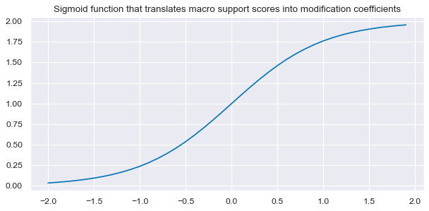
Adjustments to the strength of the trend signal based on the quantamental information captured by macro scores. The trend remains the dominant signal, but we allow quantamental information to increase the trend signal by up to 100% and to reduce it by up to zero. However, quantamental information does not “flip” the signal. The modification coefficient ensures that the adjustment remains within [0,2] interval, hence preventing extreme flips or amplifications of the trend signal.
The linear modification coefficient applied to the trend is based on the macro z-scores. The application depends on the sign of the concurrent trend signal.
-
If the trend signal is positive external strength it enhances it and external weakness reduces it. The modification coefficient uses a sigmoid function that translates the external strength score such that for a value of zero it is 1, for values of -1 and 1 it is 0.25 and 1.75 respectively and for its minimum and maximum of -3 and 3 it is 0 zero and 2 respectively.
-
If the trend signal is negative the modification coefficient depends negatively on external strength but in the same way.
This can be expressed by the following equation:
where
This means for a positive trend:
and for a negative trend:
def sigmoid(x):
    return 2 / (1 + np.exp(-2 * x))


ar = np.arange(-2, 2, 0.1)
plt.figure(figsize=(9, 4), dpi=80)
plt.plot(ar, sigmoid(ar))
plt.title(
    "Sigmoid function that translates macro support scores into modification coefficients"
)
plt.show()
# Calculate adjustment coefficients based on macro factors

macroz = factorz + ["MACRO_ZN", "MACROX_ZN", "MACROX90_ZN"]


calcs = []
for zd in macroz:
    calcs += [f"{zd}_C = ( {zd} ).applymap( lambda x: 2 / (1 + np.exp( - 2 * x)) ) "]
dfa = msp.panel_calculator(dfx, calcs=calcs, cids=cidx)
dfx = msm.update_df(dfx, dfa)

coefs = list(dfa["xcat"].unique())
# Calculate modified trend signals based on macro factors
calcs = []
for tr in eqtrendz:
for xs in macroz:
trxs = tr + "m" + xs.split("_")[0]
calcs += [f"{trxs}_C = (1 - np.sign( {tr} )) + np.sign( {tr} ) * {xs}_C"]
calcs += [f"{trxs} = {trxs}_C * {tr}"]
dfa = msp.panel_calculator(dfx, calcs=calcs, cids=cids)
dfx = msm.update_df(dfx, dfa)
eqtrendz_mod = [xc for xc in dfa["xcat"].unique() if not xc.endswith("_C")]
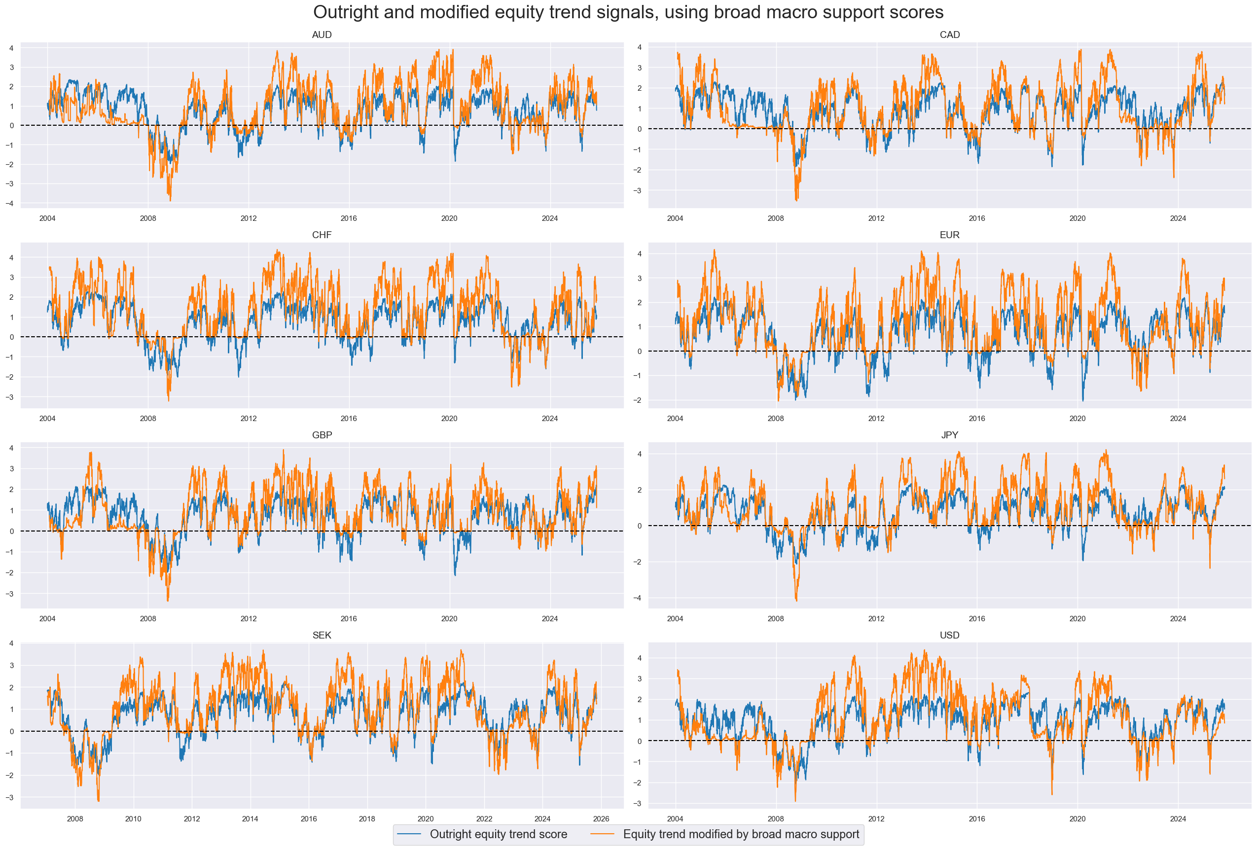
dict_names["EQXR_NSA_RTSZ"] = "Outright equity trend score"
dict_names["EQXR_NSA_RTSZmMACRO"] = "Equity trend modified by broad macro support"
dict_names["EQXR_NSA_RTSZmMACROX"] = "Equity trend modified by macro support ex carry"
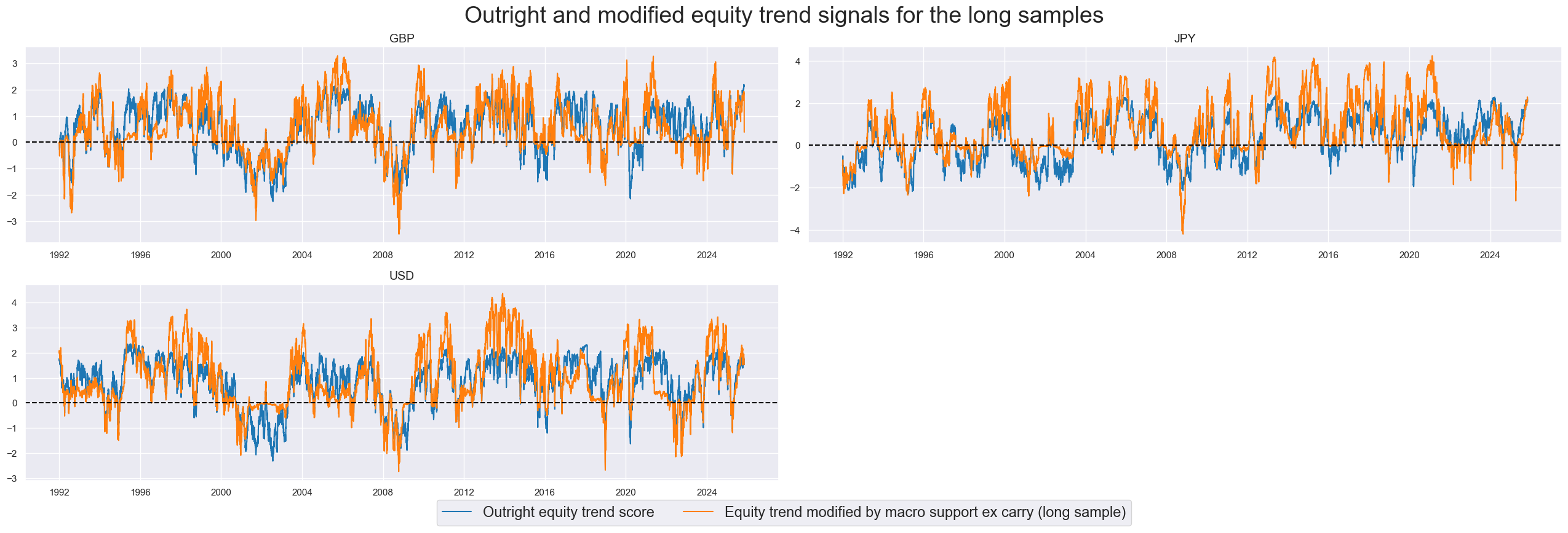
dict_names["EQXR_NSA_RTSZmMACROX90"] = "Equity trend modified by macro support ex carry (long sample)"
xcatx = ['EQXR_NSA_RTSZ', 'EQXR_NSA_RTSZmMACRO']
cidx = cids_dmeq
sdate = "2004-01-01"

msp.view_timelines(
    dfx,
    xcats=xcatx,
    cids=cidx,
    ncol=2,
    aspect=3,
    cumsum=False,
    start=sdate,
    same_y=False,
    all_xticks=True,
    legend_fontsize=17,
    title="Outright and modified equity trend signals, using broad macro support scores",
    title_fontsize=27,
    xcat_labels=dict_names,
)
xcatx = ['EQXR_NSA_RTSZ', 'EQXR_NSA_RTSZmMACROX90']
cidx = cids_dm90
sdate = "1990-01-01"

msp.view_timelines(
    dfx,
    xcats=xcatx,
    cids=cidx,
    ncol=2,
    aspect=3,
    cumsum=False,
    start=sdate,
    same_y=False,
    all_xticks=True,
    legend_fontsize=17,
    title="Outright and modified equity trend signals for the long samples",
    title_fontsize=27,
    xcat_labels=dict_names,
)
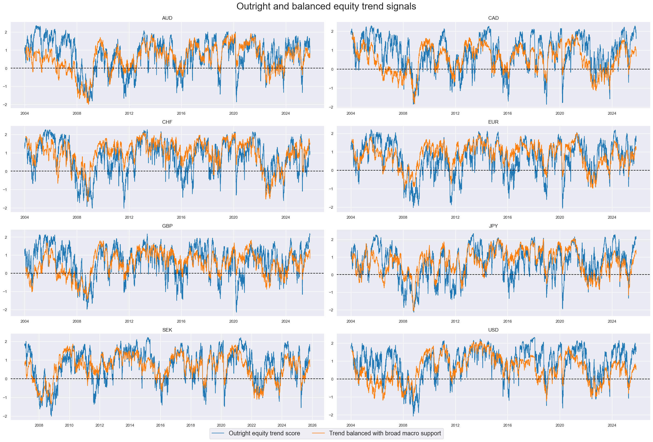
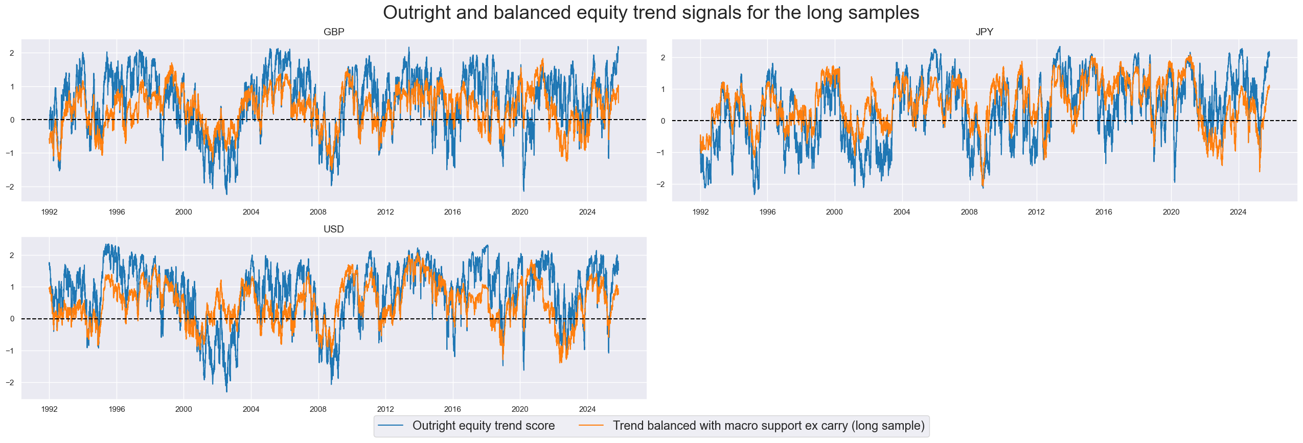
Balanced trends #
cidx = cids_dmeq

eqtrendz_bal = []
for tr in eqtrendz:
    for macro in macroz:
        xcatx = [tr, macro]
        newcat = tr + "b" + macro.split("_")[0]

        dfa = msp.linear_composite(
            df=dfx,
            xcats=xcatx,
            cids=cidx,
            complete_xcats=True,
            new_xcat=newcat,
        )
        eqtrendz_bal.append(newcat)
        dfx = msm.update_df(dfx, dfa)
dict_names["EQXR_NSA_RTSZbMACRO"] = "Trend balanced with broad macro support"
dict_names["EQXR_NSA_RTSZbMACROX"] = "Trend balanced with macro support ex carry"
dict_names["EQXR_NSA_RTSZbMACROX90"] = "Trend balanced with macro support ex carry (long sample)"
xcatx = ['EQXR_NSA_RTSZ', 'EQXR_NSA_RTSZbMACRO']
cidx = cids_dmeq
sdate = "2004-01-01"

msp.view_timelines(
    dfx,
    xcats=xcatx,
    cids=cidx,
    ncol=2,
    aspect=3,
    cumsum=False,
    start=sdate,
    same_y=False,
    all_xticks=True,
    legend_fontsize=17,
    title="Outright and balanced equity trend signals",
    title_fontsize=27,
    xcat_labels=dict_names,
)
xcatx = ['EQXR_NSA_RTSZ', 'EQXR_NSA_RTSZbMACROX90']
cidx = cids_dm90
sdate = "1990-01-01"

msp.view_timelines(
    dfx,
    xcats=xcatx,
    cids=cidx,
    ncol=2,
    aspect=3,
    cumsum=False,
    start=sdate,
    same_y=False,
    all_xticks=True,
    legend_fontsize=17,
    title="Outright and balanced equity trend signals for the long samples",
    title_fontsize=27,
    xcat_labels=dict_names,
)
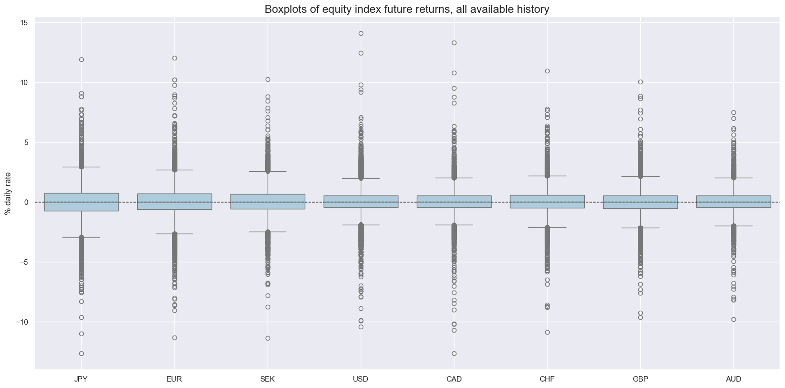
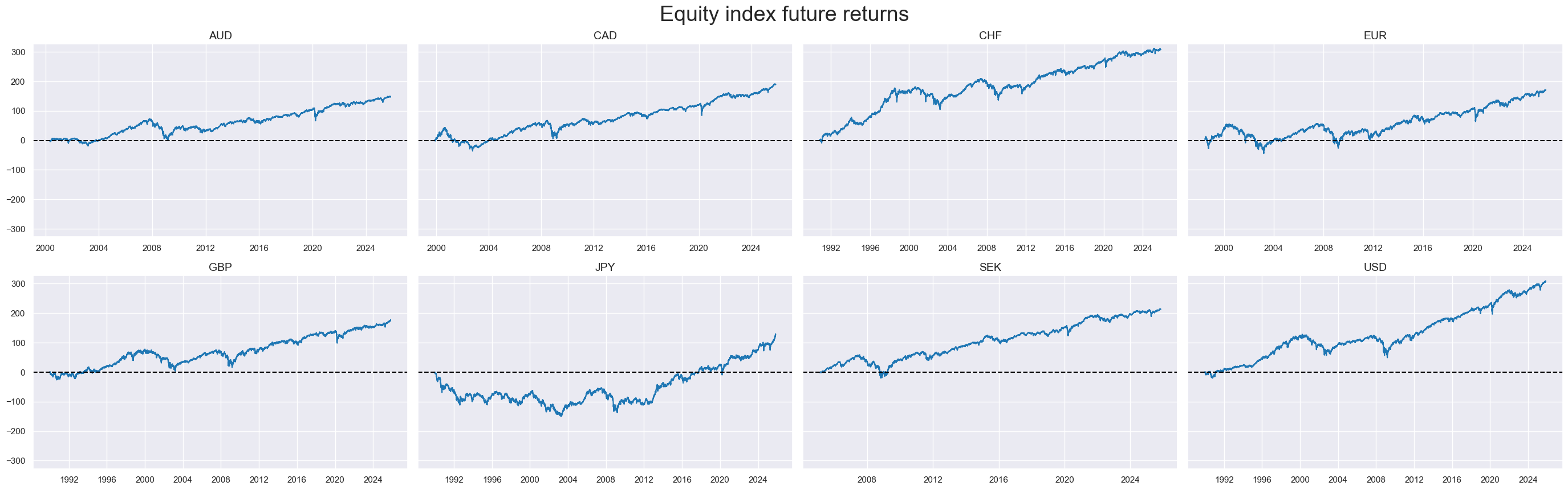
Targets review #
As target we choose standard Equity index future returns EQXR_NSA
xcatx = ["EQXR_NSA"]
cidx = cids
sdate = "1990-01-01"

msp.view_ranges(
    dfx,
    cids=cidx,
    xcats=xcatx,
    kind="box",
    sort_cids_by="std",
    ylab="% daily rate",
    start=sdate,
    title="Boxplots of equity index future returns, all available history",
)

msp.view_timelines(
    dfx,
    xcats=xcatx,
    cids=cidx,
    ncol=4,
    cumsum=True,
    start=sdate,
    same_y=True,
    size=(12, 12),
    all_xticks=True,
    title="Equity index future returns",
    title_fontsize=27,
    legend_fontsize=17,
)
xcatx = ["EQXR_NSA"]
cidx = cids

dfa = pd.DataFrame(columns=list(dfx.columns))

for xc in xcatx:
    dfaa = msp.linear_composite(
        df=dfx,
        xcats=xc,
        cids=cidx,
        complete_xcats=False,
        weights="USDGDPWGT_SA_3YMA",
        new_cid="GDM",
    )
    dfa = msm.update_df(dfa, dfaa)

dfx = msm.update_df(dfx, dfa)
Value checks #
Modified robust trends (short sample) #
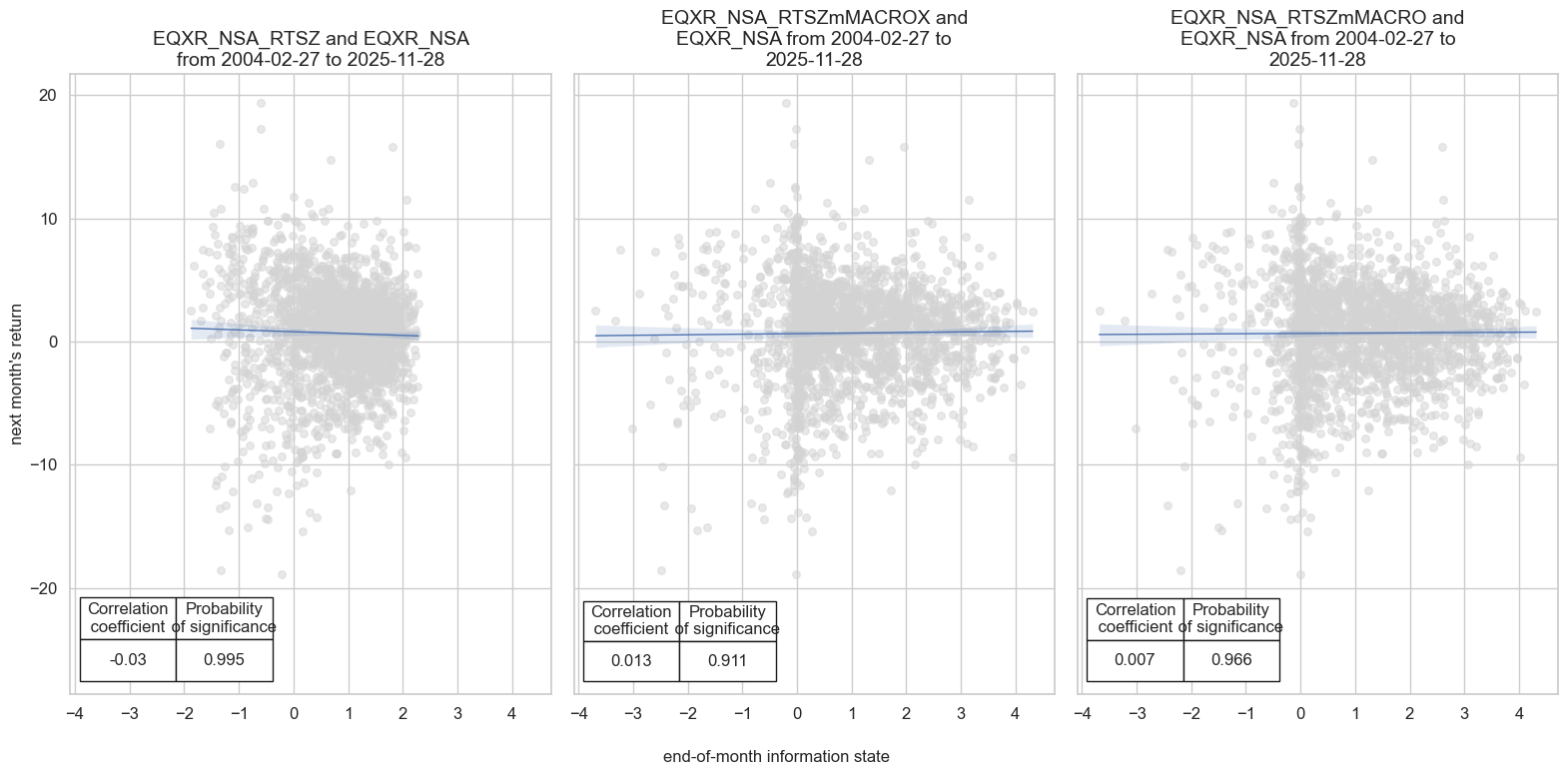
Specs and panel test #
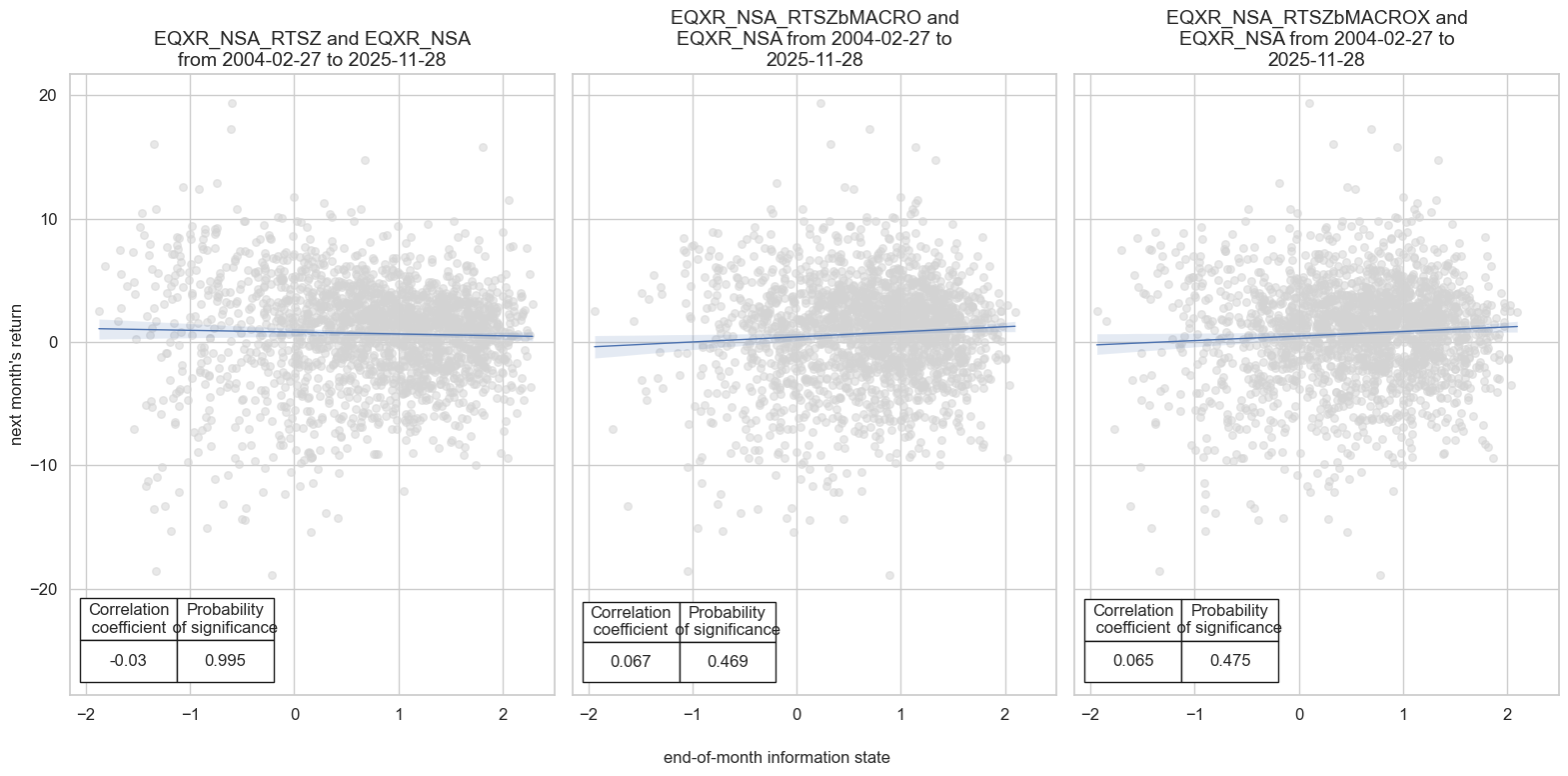
dict_m04 = {
    "sigs": ["EQXR_NSA_RTSZ", "EQXR_NSA_RTSZmMACROX", "EQXR_NSA_RTSZmMACRO"],
    "targs": ["EQXR_NSA"],
    "cidx": cids_dmeq,
    "start": "2004-01-01",
    "crs": None,
    "srr": None,
    "pnls": None,
}
dix = dict_m04

sigs = dix["sigs"]
targs = dix["targs"]
cidx = dix["cidx"]
start = dix["start"]

# Initialize the dictionary to store CategoryRelations instances

dict_cr = {}

for targ in targs:
    for sig in sigs:
        lab = sig + "_" + targ
        dict_cr[lab] = msp.CategoryRelations(
            dfx,
            xcats=[sig, targ],
            cids=cidx,
            freq="M",
            lag=1,
            xcat_aggs=["last", "sum"],
            start=start,
        )

dix["crs"] = dict_cr
# Plotting panel scatters

dix = dict_m04
dict_cr = dix["crs"]
sigs = dix["sigs"]
targs = dix["targs"]

crs = list(dict_cr.values())
crs_keys = list(dict_cr.keys())
ncol = len(sigs)
nrow = len(targs)

msv.multiple_reg_scatter(
    cat_rels=crs,
    ncol=ncol,
    nrow=nrow,
    figsize=(16, 8),
    prob_est="map",
    coef_box="lower left",
    title=None,
    subplot_titles=None,
    xlab="end-of-month information state",
    ylab="next month's return",
)
Accuracy and correlation check #
dix = dict_m04

sigs = dix["sigs"]
targ = dix["targs"][0]
cidx = dix["cidx"]
start = dix["start"]

srr = mss.SignalReturnRelations(
    dfx,
    cids=cidx,
    sigs=sigs,
    rets=targ,
    freqs="M",
    start=start,
)

dix["srr"] = srr
display(srr.signals_table().sort_index().astype("float").round(3))
| accuracy | bal_accuracy | pos_sigr | pos_retr | pos_prec | neg_prec | pearson | pearson_pval | kendall | kendall_pval | auc | ||||
|---|---|---|---|---|---|---|---|---|---|---|---|---|---|---|
| Return | Signal | Frequency | Aggregation | |||||||||||
| EQXR_NSA | EQXR_NSA_RTSZ | M | last | 0.58 | 0.506 | 0.811 | 0.622 | 0.625 | 0.388 | -0.030 | 0.174 | -0.060 | 0.000 | 0.504 |
| EQXR_NSA_RTSZmMACRO | M | last | 0.58 | 0.506 | 0.811 | 0.622 | 0.625 | 0.388 | 0.007 | 0.749 | -0.033 | 0.026 | 0.504 | |
| EQXR_NSA_RTSZmMACROX | M | last | 0.58 | 0.506 | 0.811 | 0.622 | 0.625 | 0.388 | 0.013 | 0.546 | -0.024 | 0.103 | 0.504 |
Naive PnL #
dix = dict_m04

sigx = dix["sigs"]
targ = dix["targs"][0]
cidx = dix["cidx"]
start = dix["start"]

naive_pnl = msn.NaivePnL(
    dfx,
    ret=targ,
    sigs=sigx,
    cids=cidx,
    start=start,
    bms=["USD_EQXR_NSA"],
)

for sig in sigx:
    for bias in [0, 1]:
        naive_pnl.make_pnl(
            sig,
            sig_add=bias,
            sig_op="zn_score_pan",
            thresh=2,
            rebal_freq="monthly",
            vol_scale=10,
            rebal_slip=1,
            pnl_name=sig + "_PZN" + str(bias),
        )

naive_pnl.make_long_pnl(label="Long only", vol_scale=10)

dix["pnls"] = naive_pnl

dict_names["EQXR_NSA_RTSZmMACROX_PZN0"] = "Trend modified by macro support ex carry"
dict_names["EQXR_NSA_RTSZmMACRO_PZN0"] = "Trend modified by broad macro support"
dict_names["EQXR_NSA_RTSZ_PZN0"] = "Outright trend score, no bias"

dict_names["EQXR_NSA_RTSZmMACROX_PZN1"] = "Trend modified by macro support ex carry, long only"
dict_names["EQXR_NSA_RTSZmMACRO_PZN1"] = "Trend modified by broad macro support, long only"
dict_names["EQXR_NSA_RTSZ_PZN1"] = "Outright trend score, long only"

dict_names["Long only"] = "Constant long exposure"
dix = dict_m04
sigx = dix["sigs"]
cidx = dix["cidx"]
start = dix["start"]
naive_pnl = dix["pnls"]
pnls = [s + "_PZN0" for s in sigx] # + ["Long only"]
pnls_labels = [dict_names[s] for s in pnls]
naive_pnl.plot_pnls(
pnl_cats=pnls,
pnl_cids=["ALL"],
start=start,
title="Long-short equity strategy PnL based on robust trend signals, short sample (8 countries)",
title_fontsize=18,
figsize=(17, 7),
xcat_labels=pnls_labels,
)
display(naive_pnl.evaluate_pnls(pnl_cats=pnls))
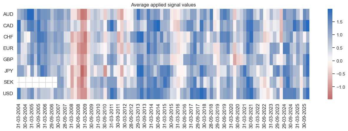
naive_pnl.signal_heatmap(pnl_name=sigx[0] + "_PZN0", freq="q", start=start, figsize=(16, 4))

| xcat | EQXR_NSA_RTSZ_PZN0 | EQXR_NSA_RTSZmMACROX_PZN0 | EQXR_NSA_RTSZmMACRO_PZN0 |
|---|---|---|---|
| Return % | 3.528684 | 4.611525 | 5.160954 |
| St. Dev. % | 10.0 | 10.0 | 10.0 |
| Sharpe Ratio | 0.352868 | 0.461153 | 0.516095 |
| Sortino Ratio | 0.49014 | 0.659749 | 0.733651 |
| Max 21-Day Draw % | -17.249515 | -11.727274 | -12.453801 |
| Max 6-Month Draw % | -20.131841 | -13.534251 | -13.833832 |
| Peak to Trough Draw % | -28.256554 | -23.062968 | -21.029793 |
| Top 5% Monthly PnL Share | 0.970533 | 0.720865 | 0.67571 |
| USD_EQXR_NSA correl | 0.015871 | 0.019718 | 0.082548 |
| Traded Months | 263 | 263 | 263 |
dix = dict_m04

sigx = dix["sigs"]
targ = dix["targs"][0]
cidx = dix["cidx"]
start = dix["start"]
naive_pnl = dix["pnls"]


pnls = [s + "_PZN1" for s in sigx] + ["Long only"]
pnls_labels = [dict_names[s] for s in pnls]

naive_pnl.plot_pnls(
    pnl_cats=pnls,
    pnl_cids=["ALL"],
    start=start,
    title="Long-biased equity index strategy PnL based on robust trend signals (short sample, 8 countries)",
    title_fontsize=18,
    figsize=(17, 7),
    xcat_labels=pnls_labels,
)

naive_pnl.plot_pnls(
    pnl_cats=pnls,
    pnl_cids=["ALL"],
    compounding=True,
    start=start,
    title="Compounding long-biased equity index strategy PnL based on robust trend signals (short sample, 8 countries)",
    title_fontsize=18,
    figsize=(17, 7),
    xcat_labels=pnls_labels,
)

display(naive_pnl.evaluate_pnls(pnl_cats=pnls))
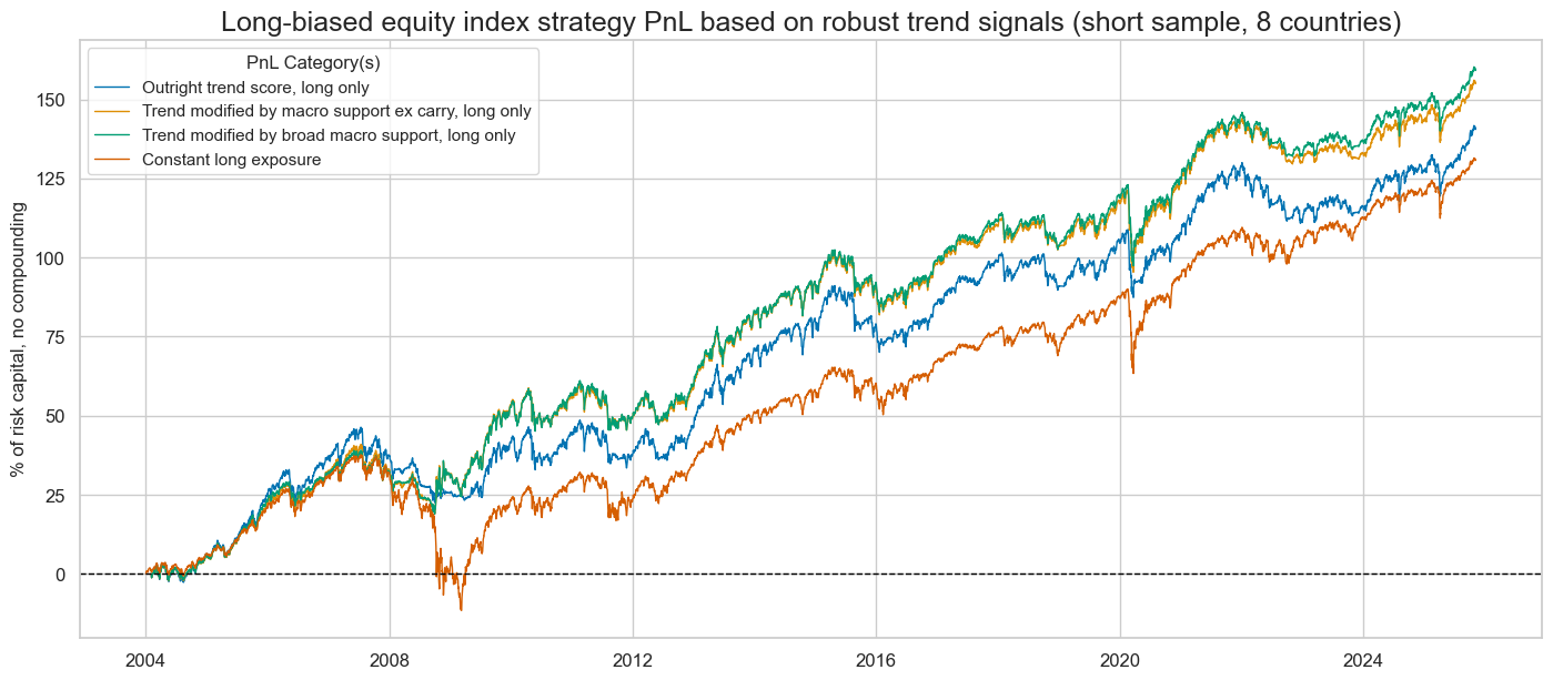
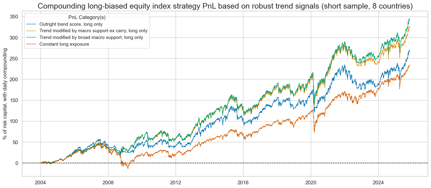
| xcat | EQXR_NSA_RTSZ_PZN1 | EQXR_NSA_RTSZmMACROX_PZN1 | EQXR_NSA_RTSZmMACRO_PZN1 | Long only |
|---|---|---|---|---|
| Return % | 6.469399 | 7.131068 | 7.323027 | 5.991095 |
| St. Dev. % | 10.0 | 10.0 | 10.0 | 10.0 |
| Sharpe Ratio | 0.64694 | 0.713107 | 0.732303 | 0.59911 |
| Sortino Ratio | 0.8831 | 0.987142 | 1.013249 | 0.822924 |
| Max 21-Day Draw % | -20.494788 | -24.963731 | -24.623618 | -25.933182 |
| Max 6-Month Draw % | -17.03438 | -16.28261 | -16.069986 | -34.370852 |
| Peak to Trough Draw % | -23.796869 | -25.964433 | -25.59586 | -49.259564 |
| Top 5% Monthly PnL Share | 0.502348 | 0.487921 | 0.474487 | 0.548609 |
| USD_EQXR_NSA correl | 0.542887 | 0.500556 | 0.516466 | 0.714698 |
| Traded Months | 263 | 263 | 263 | 263 |
Modified robust trends (long sample) #
Specs and panel test #
dict_m92 = {
    "sigs": ["EQXR_NSA_RTSZ", "EQXR_NSA_RTSZmMACROX90"],
    "targs": ["EQXR_NSA"],
    "cidx": cids_dm90,
    "start": "1992-01-01",
    "crs": None,
    "srr": None,
    "pnls": None,
}
dix = dict_m92

sigs = dix["sigs"]
targs = dix["targs"]
cidx = dix["cidx"]
start = dix["start"]

# Initialize the dictionary to store CategoryRelations instances

dict_cr = {}

for targ in targs:
    for sig in sigs:
        lab = sig + "_" + targ
        dict_cr[lab] = msp.CategoryRelations(
            dfx,
            xcats=[sig, targ],
            cids=cidx,
            freq="M",
            lag=1,
            xcat_aggs=["last", "sum"],
            start=start,
        )

dix["crs"] = dict_cr
# Plotting panel scatters

dix = dict_m92
dict_cr = dix["crs"]
sigs = dix["sigs"]
targs = dix["targs"]

crs = list(dict_cr.values())
crs_keys = list(dict_cr.keys())
ncol = len(sigs)
nrow = len(targs)

msv.multiple_reg_scatter(
    cat_rels=crs,
    ncol=ncol,
    nrow=nrow,
    figsize=(16, 8),
    prob_est="map",
    coef_box="lower left",
    title=None,
    subplot_titles=None,
    xlab="end-of-month information state",
    ylab="next month's return",
)
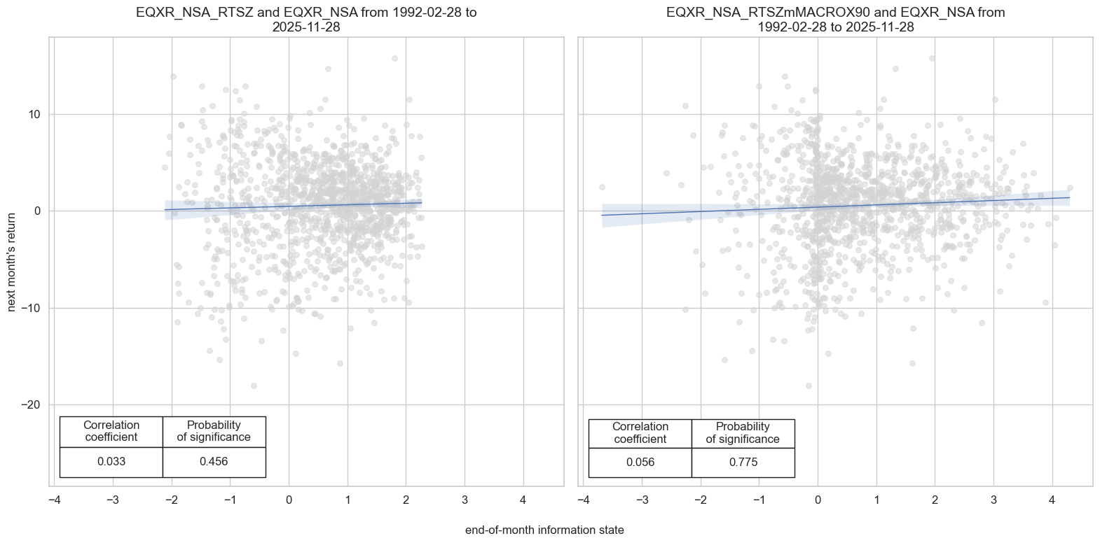
Accuracy and correlation check #
dix = dict_m92

sigs = dix["sigs"]
targs = dix["targs"]
cidx = dix["cidx"]
start = dix["start"]

srr = mss.SignalReturnRelations(
    dfx,
    cids=cidx,
    sigs=sigs,
    rets=targs[0],
    freqs="M",
    start=start,
)

dix["srr"] = srr
display(srr.signals_table().sort_index().astype("float").round(3))
| accuracy | bal_accuracy | pos_sigr | pos_retr | pos_prec | neg_prec | pearson | pearson_pval | kendall | kendall_pval | auc | ||||
|---|---|---|---|---|---|---|---|---|---|---|---|---|---|---|
| Return | Signal | Frequency | Aggregation | |||||||||||
| EQXR_NSA | EQXR_NSA_RTSZ | M | last | 0.569 | 0.523 | 0.738 | 0.608 | 0.62 | 0.426 | 0.033 | 0.245 | -0.014 | 0.463 | 0.519 |
| EQXR_NSA_RTSZmMACROX90 | M | last | 0.569 | 0.523 | 0.738 | 0.608 | 0.62 | 0.426 | 0.056 | 0.049 | 0.016 | 0.400 | 0.519 |
Naive PnL #
dix = dict_m92

sigx = dix["sigs"]
targ = dix["targs"][0]
cidx = dix["cidx"]
start = dix["start"]

naive_pnl = msn.NaivePnL(
    dfx,
    ret=targ,
    sigs=sigx,
    cids=cidx,
    start=start,
    bms=["USD_EQXR_NSA"],
)

for sig in sigx:
    for bias in [0, 1]:
        naive_pnl.make_pnl(
            sig,
            sig_add=bias,
            sig_op="zn_score_pan",
            thresh=2,
            rebal_freq="monthly",
            vol_scale=10,
            rebal_slip=1,
            pnl_name=sig + "_PZN" + str(bias),
        )

naive_pnl.make_long_pnl(label="Long only", vol_scale=10)

dix["pnls"] = naive_pnl

dict_names["EQXR_NSA_RTSZmMACROX90_PZN0"] = "Trend modified by macro support ex carry"
dict_names["EQXR_NSA_RTSZmMACROX90_PZN1"] = "Trend modified by macro support ex carry, long only"
dict_names["Long only"] = "Constant long exposure"
dix = dict_m92
sigx = dix["sigs"]
cidx = dix["cidx"]
start = dix["start"]
naive_pnl = dix["pnls"]
pnls = [s + "_PZN0" for s in sigx] # + ["Long only"]
pnls_labels = [dict_names[s] for s in pnls]
naive_pnl.plot_pnls(
pnl_cats=pnls,
pnl_cids=["ALL"],
start=start,
title="Long-short equity strategy PnL based on robust trend signals, long sample (U.S., Japan and UK)",
title_fontsize=18,
figsize=(17, 7),
xcat_labels=pnls_labels,
)
display(naive_pnl.evaluate_pnls(pnl_cats=pnls))
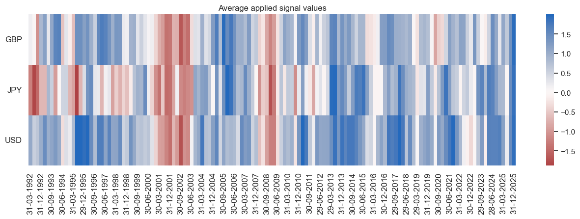
naive_pnl.signal_heatmap(pnl_name=sigx[0] + "_PZN0", freq="q", start=start, figsize=(16, 4))
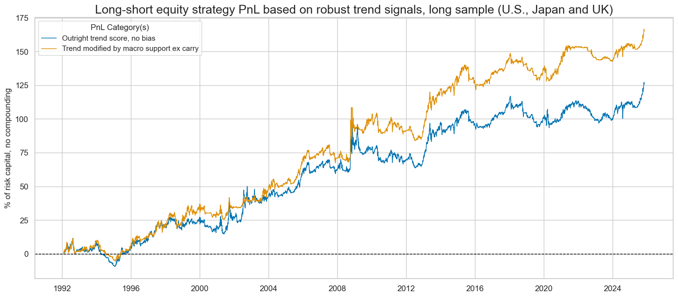
| xcat | EQXR_NSA_RTSZ_PZN0 | EQXR_NSA_RTSZmMACROX90_PZN0 |
|---|---|---|
| Return % | 3.72163 | 4.887374 |
| St. Dev. % | 10.0 | 10.0 |
| Sharpe Ratio | 0.372163 | 0.488737 |
| Sortino Ratio | 0.523293 | 0.69336 |
| Max 21-Day Draw % | -16.538491 | -14.077572 |
| Max 6-Month Draw % | -20.139674 | -16.617127 |
| Peak to Trough Draw % | -31.985569 | -24.576959 |
| Top 5% Monthly PnL Share | 1.048141 | 0.743807 |
| USD_EQXR_NSA correl | -0.016876 | 0.080418 |
| Traded Months | 406 | 406 |
[s + "_PZN1" for s in sigx] + ["Long only"]
['EQXR_NSA_RTSZ_PZN1', 'EQXR_NSA_RTSZmMACROX90_PZN1', 'Long only']
dix = dict_m92
sigx = dix["sigs"]
targ = dix["targs"][0]
cidx = dix["cidx"]
start = dix["start"]
naive_pnl = dix["pnls"]
pnls = [s + "_PZN1" for s in sigx] + ["Long only"]
pnls_labels = [dict_names[s] for s in pnls]
naive_pnl.plot_pnls(
pnl_cats=pnls,
pnl_cids=["ALL"],
start=start,
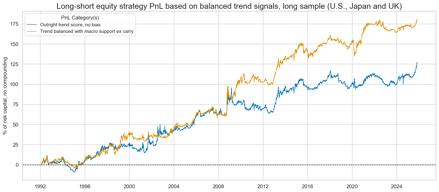
title="Long-biased equity index strategy PnL based on robust trend signals, long sample (U.S., Japan and UK)",
title_fontsize=18,
figsize=(17, 7),
xcat_labels=pnls_labels,
)
naive_pnl.plot_pnls(
pnl_cats=pnls,
pnl_cids=["ALL"],
compounding=True,
start=start,
title="Compounding long-biased equity index strategy PnL based on robust trend signals, long sample (U.S., Japan and UK)",
title_fontsize=18,
figsize=(17, 7),
xcat_labels=pnls_labels,
)
display(naive_pnl.evaluate_pnls(pnl_cats=pnls))
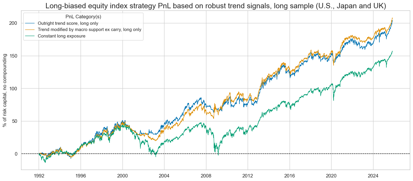
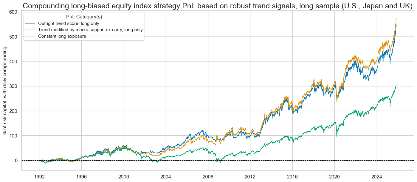
| xcat | EQXR_NSA_RTSZ_PZN1 | EQXR_NSA_RTSZmMACROX90_PZN1 | Long only |
|---|---|---|---|
| Return % | 6.001115 | 6.123128 | 4.616036 |
| St. Dev. % | 10.0 | 10.0 | 10.0 |
| Sharpe Ratio | 0.600112 | 0.612313 | 0.461604 |
| Sortino Ratio | 0.831972 | 0.861031 | 0.643966 |
| Max 21-Day Draw % | -15.493662 | -20.961533 | -24.670135 |
| Max 6-Month Draw % | -17.408402 | -16.659535 | -35.230715 |
| Peak to Trough Draw % | -22.943567 | -29.48868 | -50.960851 |
| Top 5% Monthly PnL Share | 0.545808 | 0.582392 | 0.67632 |
| USD_EQXR_NSA correl | 0.478236 | 0.491261 | 0.706153 |
| Traded Months | 407 | 407 | 407 |
Balanced robust trends (short sample) #
Specs and panel test #
dict_b04 = {
    "sigs": ["EQXR_NSA_RTSZ", "EQXR_NSA_RTSZbMACRO", "EQXR_NSA_RTSZbMACROX"],
    "targs": ["EQXR_NSA"],
    "cidx": cids_dmeq,
    "start": "2004-01-01",
    "crs": None,
    "srr": None,
    "pnls": None,
}
dix = dict_b04

sigs = dix["sigs"]
targs = dix["targs"]
cidx = dix["cidx"]
start = dix["start"]

# Initialize the dictionary to store CategoryRelations instances

dict_cr = {}

for targ in targs:
    for sig in sigs:
        lab = sig + "_" + targ
        dict_cr[lab] = msp.CategoryRelations(
            dfx,
            xcats=[sig, targ],
            cids=cidx,
            freq="M",
            lag=1,
            xcat_aggs=["last", "sum"],
            start=start,
        )

dix["crs"] = dict_cr
# Plotting panel scatters

dix = dict_b04
dict_cr = dix["crs"]
sigs = dix["sigs"]
targs = dix["targs"]

crs = list(dict_cr.values())
crs_keys = list(dict_cr.keys())
ncol = len(sigs)
nrow = len(targs)

msv.multiple_reg_scatter(
    cat_rels=crs,
    ncol=ncol,
    nrow=nrow,
    figsize=(16, 8),
    prob_est="map",
    coef_box="lower left",
    title=None,
    subplot_titles=None,
    xlab="end-of-month information state",
    ylab="next month's return",
)
Accuracy and correlation check #
dix = dict_b04

sigs = dix["sigs"]
targ = dix["targs"][0]
cidx = dix["cidx"]
start = dix["start"]

srr = mss.SignalReturnRelations(
    dfx,
    cids=cidx,
    sigs=sigs,
    rets=targ,
    freqs="M",
    start=start,
)

dix["srr"] = srr
display(srr.signals_table().sort_index().astype("float").round(3))
| accuracy | bal_accuracy | pos_sigr | pos_retr | pos_prec | neg_prec | pearson | pearson_pval | kendall | kendall_pval | auc | ||||
|---|---|---|---|---|---|---|---|---|---|---|---|---|---|---|
| Return | Signal | Frequency | Aggregation | |||||||||||
| EQXR_NSA | EQXR_NSA_RTSZ | M | last | 0.580 | 0.506 | 0.811 | 0.622 | 0.625 | 0.388 | -0.030 | 0.174 | -0.060 | 0.000 | 0.504 |
| EQXR_NSA_RTSZbMACRO | M | last | 0.606 | 0.549 | 0.814 | 0.622 | 0.640 | 0.457 | 0.067 | 0.002 | 0.011 | 0.457 | 0.531 | |
| EQXR_NSA_RTSZbMACROX | M | last | 0.601 | 0.549 | 0.773 | 0.622 | 0.645 | 0.454 | 0.065 | 0.003 | 0.015 | 0.322 | 0.537 |
Naive PnL #
dix = dict_b04

sigx = dix["sigs"]
targ = dix["targs"][0]
cidx = dix["cidx"]
start = dix["start"]

naive_pnl = msn.NaivePnL(
    dfx,
    ret=targ,
    sigs=sigx,
    cids=cidx,
    start=start,
    bms=["USD_EQXR_NSA"],
)

for sig in sigx:
    for bias in [0, 1]:
        naive_pnl.make_pnl(
            sig,
            sig_add=bias,
            sig_op="zn_score_pan",
            thresh=2,
            rebal_freq="monthly",
            vol_scale=10,
            rebal_slip=1,
            pnl_name=sig + "_PZN" + str(bias),
        )

naive_pnl.make_long_pnl(label="Long only", vol_scale=10)

dix["pnls"] = naive_pnl

dict_names["EQXR_NSA_RTSZbMACROX_PZN0"] = "Trend balanced with macro support ex carry"
dict_names["EQXR_NSA_RTSZbMACRO_PZN0"] = "Trend balanced with broad macro support"

dict_names["EQXR_NSA_RTSZbMACROX_PZN1"] = "Trend balanced with macro support ex carry, long bias"
dict_names["EQXR_NSA_RTSZbMACRO_PZN1"] = "Trend balanced with broad macro support, long bias"


dix["pnls"] = naive_pnl
dix = dict_b04

sigx = dix["sigs"]
targ = dix["targs"][0]
cidx = dix["cidx"]
start = dix["start"]
naive_pnl = dix["pnls"]


pnls = [s + "_PZN0" for s in sigx] # + ["Long only"]
pnls_labels = [dict_names[s] for s in pnls]

naive_pnl.plot_pnls(
    pnl_cats=pnls,
    pnl_cids=["ALL"],
    start=start,
    title="Long-short equity strategy PnL based on balanced trend signals, short sample (8 countries)",
    title_fontsize=18,
    figsize=(17, 7),
    xcat_labels=pnls_labels,
)

display(naive_pnl.evaluate_pnls(pnl_cats=pnls))

naive_pnl.signal_heatmap(pnl_name=sigx[0] + "_PZN0", freq="q", start=start, figsize=(16, 4))
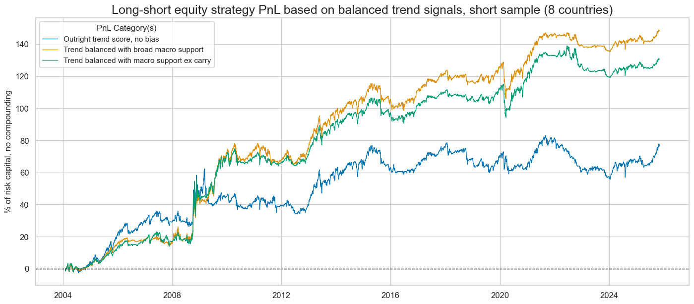
| xcat | EQXR_NSA_RTSZ_PZN0 | EQXR_NSA_RTSZbMACRO_PZN0 | EQXR_NSA_RTSZbMACROX_PZN0 |
|---|---|---|---|
| Return % | 3.528684 | 6.81049 | 5.996592 |
| St. Dev. % | 10.0 | 10.0 | 10.0 |
| Sharpe Ratio | 0.352868 | 0.681049 | 0.599659 |
| Sortino Ratio | 0.49014 | 0.97138 | 0.861213 |
| Max 21-Day Draw % | -17.249515 | -22.070219 | -19.942102 |
| Max 6-Month Draw % | -20.131841 | -14.347515 | -13.539116 |
| Peak to Trough Draw % | -28.256554 | -23.008054 | -21.224042 |
| Top 5% Monthly PnL Share | 0.970533 | 0.592503 | 0.674703 |
| USD_EQXR_NSA correl | 0.015871 | 0.189461 | 0.081289 |
| Traded Months | 263 | 263 | 263 |
Balanced robust trends (long sample) #
Specs and panel test #
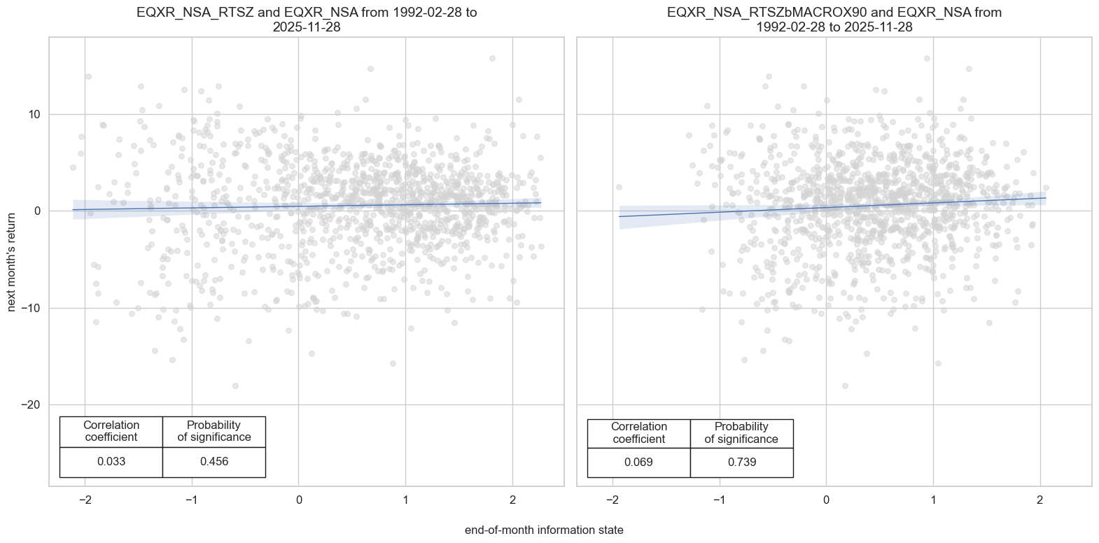
dict_b92 = {
    "sigs": ["EQXR_NSA_RTSZ", "EQXR_NSA_RTSZbMACROX90"],
    "targs": ["EQXR_NSA"],
    "cidx": cids_dm90,
    "start": "1992-01-01",
    "crs": None,
    "srr": None,
    "pnls": None,
}
dix = dict_b92

sigs = dix["sigs"]
targs = dix["targs"]
cidx = dix["cidx"]
start = dix["start"]

# Initialize the dictionary to store CategoryRelations instances

dict_cr = {}

for targ in targs:
    for sig in sigs:
        lab = sig + "_" + targ
        dict_cr[lab] = msp.CategoryRelations(
            dfx,
            xcats=[sig, targ],
            cids=cidx,
            freq="M",
            lag=1,
            xcat_aggs=["last", "sum"],
            start=start,
        )

dix["crs"] = dict_cr
# Plotting panel scatters

dix = dict_b92
dict_cr = dix["crs"]
sigs = dix["sigs"]
targs = dix["targs"]

crs = list(dict_cr.values())
crs_keys = list(dict_cr.keys())
ncol = len(sigs)
nrow = len(targs)

msv.multiple_reg_scatter(
    cat_rels=crs,
    ncol=ncol,
    nrow=nrow,
    figsize=(16, 8),
    prob_est="map",
    coef_box="lower left",
    title=None,
    subplot_titles=None,
    xlab="end-of-month information state",
    ylab="next month's return",
)
Accuracy and correlation check #
dix = dict_b92

sigs = dix["sigs"]
targs = dix["targs"]
cidx = dix["cidx"]
start = dix["start"]

srr = mss.SignalReturnRelations(
    dfx,
    cids=cidx,
    sigs=sigs,
    rets=targs[0],
    freqs="M",
    start=start,
)

dix["srr"] = srr
display(srr.signals_table().sort_index().astype("float").round(3))
| accuracy | bal_accuracy | pos_sigr | pos_retr | pos_prec | neg_prec | pearson | pearson_pval | kendall | kendall_pval | auc | ||||
|---|---|---|---|---|---|---|---|---|---|---|---|---|---|---|
| Return | Signal | Frequency | Aggregation | |||||||||||
| EQXR_NSA | EQXR_NSA_RTSZ | M | last | 0.569 | 0.523 | 0.738 | 0.608 | 0.620 | 0.426 | 0.033 | 0.245 | -0.014 | 0.463 | 0.519 |
| EQXR_NSA_RTSZbMACROX90 | M | last | 0.575 | 0.528 | 0.749 | 0.608 | 0.622 | 0.435 | 0.069 | 0.016 | 0.034 | 0.077 | 0.522 |
Naive PnL #
dix = dict_b92

sigx = dix["sigs"]
targ = dix["targs"][0]
cidx = dix["cidx"]
start = dix["start"]

naive_pnl = msn.NaivePnL(
    dfx,
    ret=targ,
    sigs=sigx,
    cids=cidx,
    start=start,
    bms=["USD_EQXR_NSA"],
)

for sig in sigx:
    for bias in [0, 1]:
        naive_pnl.make_pnl(
            sig,
            sig_add=bias,
            sig_op="zn_score_pan",
            thresh=2,
            rebal_freq="monthly",
            vol_scale=10,
            rebal_slip=1,
            pnl_name=sig + "_PZN" + str(bias),
        )

naive_pnl.make_long_pnl(label="Long only", vol_scale=10)

dix["pnls"] = naive_pnl

dict_names["EQXR_NSA_RTSZbMACROX90_PZN0"] = "Trend balanced with macro support ex carry"
dict_names["EQXR_NSA_RTSZbMACROX90_PZN1"] = "Trend balanced with macro support ex carry, long bias"
dix = dict_b92

sigx = dix["sigs"]
targ = dix["targs"][0]
cidx = dix["cidx"]
start = dix["start"]
naive_pnl = dix["pnls"]


pnls = [s + "_PZN0" for s in sigx] # + ["Long only"]
pnls_labels = [dict_names[s] for s in pnls]

naive_pnl.plot_pnls(
    pnl_cats=pnls,
    pnl_cids=["ALL"],
    start=start,
    title="Long-short equity strategy PnL based on balanced trend signals, long sample (U.S., Japan and UK)",
    title_fontsize=18,
    figsize=(17, 7),
    xcat_labels=pnls_labels,
)

display(naive_pnl.evaluate_pnls(pnl_cats=pnls))

naive_pnl.signal_heatmap(pnl_name=sigx[0] + "_PZN0", freq="q", start=start, figsize=(16, 4))
| xcat | EQXR_NSA_RTSZ_PZN0 | EQXR_NSA_RTSZbMACROX90_PZN0 |
|---|---|---|
| Return % | 3.72163 | 5.32993 |
| St. Dev. % | 10.0 | 10.0 |
| Sharpe Ratio | 0.372163 | 0.532993 |
| Sortino Ratio | 0.523293 | 0.757928 |
| Max 21-Day Draw % | -16.538491 | -18.999092 |
| Max 6-Month Draw % | -20.139674 | -16.586622 |
| Peak to Trough Draw % | -31.985569 | -26.488982 |
| Top 5% Monthly PnL Share | 1.048141 | 0.735054 |
| USD_EQXR_NSA correl | -0.016876 | 0.138096 |
| Traded Months | 406 | 406 |
dix = dict_b92

sigx = dix["sigs"]
targ = dix["targs"][0]
cidx = dix["cidx"]
start = dix["start"]
naive_pnl = dix["pnls"]


pnls = [s + "_PZN1" for s in sigx] + ["Long only"]
pnls_labels = [dict_names[s] for s in pnls]

naive_pnl.plot_pnls(
    pnl_cats=pnls,
    pnl_cids=["ALL"],
    start=start,
    title="Long-biased equity index strategy PnL based on balanced trend signals, long sample (U.S., Japan and UK)",
    title_fontsize=18,
    figsize=(17, 7),
    xcat_labels=pnls_labels,
)

naive_pnl.plot_pnls(
    pnl_cats=pnls,
    pnl_cids=["ALL"],
    compounding=True,
    start=start,
    title="Compounding long-biased equity index strategy PnL based on balanced trend signals, long sample (U.S., Japan and UK)",
    title_fontsize=18,
    figsize=(17, 7),
    xcat_labels=pnls_labels,
)

display(naive_pnl.evaluate_pnls(pnl_cats=pnls))

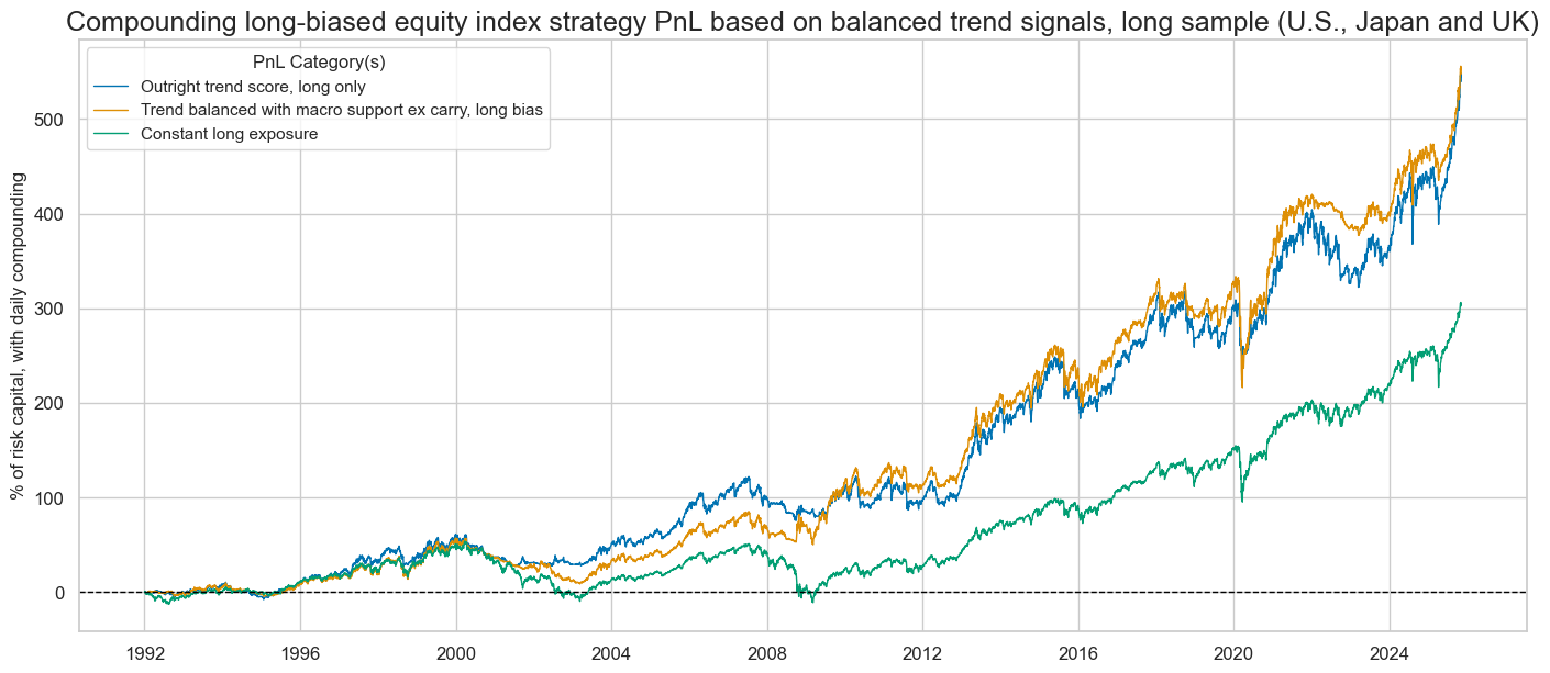
| xcat | EQXR_NSA_RTSZ_PZN1 | EQXR_NSA_RTSZbMACROX90_PZN1 | Long only |
|---|---|---|---|
| Return % | 6.001115 | 6.038253 | 4.616036 |
| St. Dev. % | 10.0 | 10.0 | 10.0 |
| Sharpe Ratio | 0.600112 | 0.603825 | 0.461604 |
| Sortino Ratio | 0.831972 | 0.851594 | 0.643966 |
| Max 21-Day Draw % | -15.493662 | -29.032184 | -24.670135 |
| Max 6-Month Draw % | -17.408402 | -22.667801 | -35.230715 |
| Peak to Trough Draw % | -22.943567 | -35.90696 | -50.960851 |
| Top 5% Monthly PnL Share | 0.545808 | 0.624878 | 0.67632 |
| USD_EQXR_NSA correl | 0.478236 | 0.509069 | 0.706153 |
| Traded Months | 407 | 407 | 407 |
Checks #
Specs and panel test #
eqtrendz_bal
['EQXR_NSA_RTSZbXSPEND',
 'EQXR_NSA_RTSZbXINF',
 'EQXR_NSA_RTSZbLIQINT',
 'EQXR_NSA_RTSZbXCRR',
 'EQXR_NSA_RTSZbMACRO',
 'EQXR_NSA_RTSZbMACROX',
 'EQXR_NSA_RTSZbMACROX90']
tests = [
    "EQXR_NSA_RTSZbXSPEND",
    "EQXR_NSA_RTSZbXINF",
    "EQXR_NSA_RTSZbMACROX90",
]

dict_test = {
    "sigs": ["EQXR_NSA_RTSZ"] + tests,
    "targs": ["EQXR_NSA"],
    "cidx": cids_dm90,
    "start": "1992-01-01",
    "crs": None,
    "srr": None,
    "pnls": None,
}
dix = dict_test

sigs = dix["sigs"]
targs = dix["targs"]
cidx = dix["cidx"]
start = dix["start"]

# Initialize the dictionary to store CategoryRelations instances

dict_cr = {}

for targ in targs:
    for sig in sigs:
        lab = sig + "_" + targ
        dict_cr[lab] = msp.CategoryRelations(
            dfx,
            xcats=[sig, targ],
            cids=cidx,
            freq="M",
            lag=1,
            xcat_aggs=["last", "sum"],
            start=start,
        )

dix["crs"] = dict_cr
dix = dict_test
dict_cr = dix["crs"]
sigs = dix["sigs"]
targs = dix["targs"]

crs = list(dict_cr.values())
crs_keys = list(dict_cr.keys())
ncol = 2
nrow = 2

msv.multiple_reg_scatter(
    cat_rels=crs,
    ncol=ncol,
    nrow=nrow,
    figsize=(15, 15),
    prob_est="map",
    coef_box="lower left",
    title=None,
    subplot_titles=None,
    xlab="end-of-month information state",
    ylab="next month's return",
)

Accuracy and correlation check #
dix = dict_test

sigs = dix["sigs"]
targs = dix["targs"]
cidx = dix["cidx"]
start = dix["start"]

srr = mss.SignalReturnRelations(
    dfx,
    cids=cidx,
    sigs=sigs,
    rets=targs[0],
    freqs="M",
    start=start,
)

dix["srr"] = srr
display(srr.signals_table().sort_index().astype("float").round(3))
| accuracy | bal_accuracy | pos_sigr | pos_retr | pos_prec | neg_prec | pearson | pearson_pval | kendall | kendall_pval | auc | ||||
|---|---|---|---|---|---|---|---|---|---|---|---|---|---|---|
| Return | Signal | Frequency | Aggregation | |||||||||||
| EQXR_NSA | EQXR_NSA_RTSZ | M | last | 0.569 | 0.523 | 0.738 | 0.608 | 0.620 | 0.426 | 0.033 | 0.245 | -0.014 | 0.463 | 0.519 |
| EQXR_NSA_RTSZbMACROX90 | M | last | 0.575 | 0.528 | 0.749 | 0.608 | 0.622 | 0.435 | 0.069 | 0.016 | 0.034 | 0.077 | 0.522 | |
| EQXR_NSA_RTSZbXINF | M | last | 0.578 | 0.541 | 0.706 | 0.608 | 0.631 | 0.450 | 0.068 | 0.018 | 0.021 | 0.268 | 0.535 | |
| EQXR_NSA_RTSZbXSPEND | M | last | 0.560 | 0.525 | 0.680 | 0.607 | 0.623 | 0.426 | 0.035 | 0.233 | 0.006 | 0.749 | 0.523 |