FX trading signals and regression-based learning #
This notebook illustrates the points discussed in the post “FX trading signals and regression-based learning” on the Macrosynergy website. It demonstrates how regression-based statistical learning helps build trading signals from multiple candidate constituents. The method optimizes models and hyperparameters sequentially and produces point-in-time signals for backtesting and live trading. This post applies regression-based learning to a selection of macro trading factors for developed market FX trading, using a novel cross-validation method for expanding panel data. Sequentially optimized models consider nine theoretically valid macro trend indicators to predict FX forward returns. The learning process has delivered significant predictors of returns and consistent positive PnL generation for over 20 years. The most important macro-FX signals, in the long run, have been relative labor market trends, manufacturing business sentiment changes, inflation expectations, and terms of trade dynamics.
The notebook is organized into three main sections:
-
Get Packages and JPMaQS Data: This section is dedicated to installing and importing the necessary Python packages for the analysis. It includes standard Python libraries like pandas and seaborn, as well as the
scikit-learnpackage and the specializedmacrosynergypackage. -
Transformations and Checks: In this part, the notebook conducts data calculations and transformations to derive relevant signals and targets for the analysis. This involves constructing simple linear composite indicators, means, relative values, etc.
-
Actual regression-based learning: , employing the learning module of
macrosynergypackage for LinearRegression() fromscikit-learnpackage defining hyperparameter grid, employed models, cross-validation splits, optimization criteria, etc. -
Value checks and comparison of conceptual parity signal with OLS based learning signals. The comparison is performed using standard performance metrics, as well as calculating naive PnLs (Profit and Loss) for simple relative trading strategies based on both risk parity and OLS based learning signals.
-
Alternative models of regression-based learning explores additional models: Regularized linear model (elastic net), Sign-weighted linear regression, Time-weighted linear regression - using the standard performance metrics with naive PnL calculations.
Get packages and JPMaQS data #
import os
import numpy as np
import pandas as pd

from sklearn.pipeline import Pipeline
from sklearn.linear_model import LinearRegression, ElasticNet

from sklearn.metrics import (
    make_scorer,
    r2_score,
)

import macrosynergy.management as msm
import macrosynergy.panel as msp
import macrosynergy.pnl as msn
import macrosynergy.signal as mss
import macrosynergy.learning as msl
import macrosynergy.visuals as msv

from macrosynergy.download import JPMaQSDownload

import warnings

warnings.simplefilter("ignore")
# Cross-sections of interest - FX
cids_g3 = ["EUR", "JPY", "USD"]  # DM large currency areas
cids_dmfx = ["AUD", "CAD", "CHF", "GBP", "NOK", "NZD", "SEK"]  # DM small currency areas

cids_dm = cids_g3 + cids_dmfx
cids = cids_dm

cids_eur = ["CHF", "NOK", "SEK"]  # trading against EUR
cids_eud = ["GBP"]  # trading against EUR and USD
cids_usd = list(set(cids_dmfx) - set(cids_eur + cids_eud))  # trading against USD
# Quantamental features of interest

ir = [
    "RIR_NSA",
]

ctots = [
    "CTOT_NSA_P1M1ML12",
    "CTOT_NSA_P1M12ML1",
    "CTOT_NSA_P1W4WL1",
]

surv = [
    "MBCSCORE_SA_D3M3ML3",
    "MBCSCORE_SA_D1Q1QL1",
    "MBCSCORE_SA_D6M6ML6",
    "MBCSCORE_SA_D2Q2QL2",
]

ppi = [
    "PGDPTECH_SA_P1M1ML12_3MMA",
]

gdps = [
    "INTRGDP_NSA_P1M1ML12_3MMA",
]

emp = [
    "UNEMPLRATE_SA_D3M3ML3",
    "UNEMPLRATE_SA_D6M6ML6",
    "UNEMPLRATE_SA_D1Q1QL1",
    "UNEMPLRATE_SA_D2Q2QL2",
    "UNEMPLRATE_NSA_3MMA_D1M1ML12",
    "UNEMPLRATE_NSA_D1Q1QL4",
]

iip = [
    "IIPLIABGDP_NSA",
]

cpi = [
    "CPIXFE_SA_P1M1ML12",
    "CPIXFE_SJA_P3M3ML3AR",
    "CPIXFE_SJA_P6M6ML6AR",
    "INFE1Y_JA",
    "INFE2Y_JA",
    "INFE5Y_JA",
]

tots = ctots

main = tots + gdps + surv + ir + emp + iip + ppi + cpi

adds = [
    "INFTEFF_NSA",
]

mkts = [
    "FXTARGETED_NSA",
    "FXUNTRADABLE_NSA",
]

rets = [
    "FXXR_VT10",
]

xcats = main + mkts + rets + adds

# Resultant tickers for download

single_tix = ["USD_GB10YXR_NSA", "EUR_FXXR_NSA", "USD_EQXR_NSA"]
tickers = [cid + "_" + xcat for cid in cids for xcat in xcats] + single_tix
JPMaQS indicators are conveniently grouped into six main categories: Economic Trends, Macroeconomic balance sheets, Financial conditions, Shocks and risk measures, Stylized trading factors, and Generic returns. Each indicator has a separate page with notes, description, availability, statistical measures, and timelines for main currencies. The description of each JPMaQS category is available under the Macro quantamental academy . For tickers used in this notebook see Real short-term interest rates , Terms-of-trade , Manufacturing confidence scores , Producer price inflation , Intuitive GDP growth estimates , Labor market dynamics , International investment position , Consistent core CPI trends , FX forward returns , and FX tradeability and flexibility . JPMaQS indicators are conveniently grouped into six main categories: Economic Trends, Macroeconomic balance sheets, Financial conditions, Shocks and risk measures, Stylized trading factors, and Generic returns. Each indicator has a separate page with notes, description, availability, statistical measures, and timelines for main currencies. The description of each JPMaQS category is available under Macro quantamental academy . For tickers used in this notebook see Real short-term interest rates , Terms-of-trade , Manufacturing confidence scores , Producer price inflation , Intuitive GDP growth estimates , Labor market dynamics , International investment position , Consistent core CPI trends , Inflation expectations , Inflation targets , FX forward returns , and FX tradeability and flexibility .
In this notebook, we introduce several lists of currencies for the sake of convenience in our subsequent analysis:
-
cids_g3represents the 3 largest developed market currencies. -
cids_dmfxrepresents DM small currency areas. -
cids_eurtrading against EUR. -
cids_eudtrading against EUR and USD -
cids_usdtrading against USD
The JPMaQS indicators we consider are downloaded using the J.P. Morgan Dataquery API interface within the
macrosynergy
package. This is done by specifying ticker strings, formed by appending an indicator category code
DB(JPMAQS,<cross_section>_<category>,<info>)
, where
value
giving the latest available values for the indicator
eop_lag
referring to days elapsed since the end of the observation period
mop_lag
referring to the number of days elapsed since the mean observation period
grade
denoting a grade of the observation, giving a metric of real-time information quality.
After instantiating the
JPMaQSDownload
class within the
macrosynergy.download
module, one can use the
download(tickers,start_date,metrics)
method to easily download the necessary data, where
tickers
is an array of ticker strings,
start_date
is the first collection date to be considered and
metrics
is an array comprising the times series information to be downloaded. For more information see
here
# Download series from J.P. Morgan DataQuery by tickers

start_date = "1990-01-01"
end_date = None

# Retrieve credentials

client_id = os.getenv("DQ_CLIENT_ID")  # Replace with own client ID
client_secret = os.getenv("DQ_CLIENT_SECRET")  # Replace with own secret
proxy = {
    # "https": "https://example.com:port",
}

# Download from DataQuery

downloader = JPMaQSDownload(client_id=client_id, client_secret=client_secret, proxy=proxy)
df = downloader.download(
    tickers=tickers,
    start_date=start_date,
    end_date=end_date,
    metrics=["value"],
    suppress_warning=True,
    show_progress=True,
)

dfx = df.copy()
dfx.info()
Downloading data from JPMaQS.
Timestamp UTC:  2024-12-03 16:20:54
Connection successful!
Requesting data: 100%|█████████████████████████████████████████████████████████████████| 14/14 [00:02<00:00,  4.71it/s]
Downloading data: 100%|████████████████████████████████████████████████████████████████| 14/14 [00:11<00:00,  1.21it/s]
Some expressions are missing from the downloaded data. Check logger output for complete list.
53 out of 273 expressions are missing. To download the catalogue of all available expressions and filter the unavailable expressions, set `get_catalogue=True` in the call to `JPMaQSDownload.download()`.
Some dates are missing from the downloaded data.
2 out of 9114 dates are missing.
<class 'pandas.core.frame.DataFrame'>
RangeIndex: 1649099 entries, 0 to 1649098
Data columns (total 4 columns):
 #   Column     Non-Null Count    Dtype
---  ------     --------------    -----
 0   real_date  1649099 non-null  datetime64[ns]
 1   cid        1649099 non-null  object
 2   xcat       1649099 non-null  object
 3   value      1649099 non-null  float64
dtypes: datetime64[ns](1), float64(1), object(2)
memory usage: 50.3+ MB
Availability and blacklisting #
Renaming #
Rename quarterly tickers to roughly equivalent monthly tickers to simplify subsequent operations.
dict_repl = {
    "UNEMPLRATE_NSA_D1Q1QL4": "UNEMPLRATE_NSA_3MMA_D1M1ML12",
    "UNEMPLRATE_SA_D1Q1QL1": "UNEMPLRATE_SA_D3M3ML3",
    "UNEMPLRATE_SA_D2Q2QL2": "UNEMPLRATE_SA_D6M6ML6",
    "MBCSCORE_SA_D1Q1QL1": "MBCSCORE_SA_D3M3ML3",
    "MBCSCORE_SA_D2Q2QL2": "MBCSCORE_SA_D6M6ML6",
}

for key, value in dict_repl.items():
    dfx["xcat"] = dfx["xcat"].str.replace(key, value)
Check availability #
Prior to commencing any analysis, it is crucial to evaluate the accessibility of data. This evaluation serves several purposes, including identifying potential data gaps or constraints within the dataset. Such gaps can significantly influence the trustworthiness and accuracy of the analysis. Moreover, it aids in verifying that ample observations are accessible for each chosen category and cross-section. Additionally, it assists in establishing suitable timeframes for conducting the analysis.
xcatx = cpi + ppi + ir
msm.check_availability(df=dfx, xcats=xcatx, cids=cids, missing_recent=False)

xcatx = surv + emp
msm.check_availability(df=dfx, xcats=xcatx, cids=cids, missing_recent=False)

xcatx = gdps
msm.check_availability(df=dfx, xcats=xcatx, cids=cids, missing_recent=False)

xcatx = ctots
msm.check_availability(df=dfx, xcats=xcatx, cids=cids, missing_recent=False)

xcatx = iip
msm.check_availability(df=dfx, xcats=xcatx, cids=cids, missing_recent=False)

Blacklisting #
Identifying and isolating periods of official exchange rate targets, illiquidity, or convertibility-related distortions in FX markets is the first step in creating an FX trading strategy. These periods can significantly impact the behavior and dynamics of currency markets, and failing to account for them can lead to inaccurate or misleading findings. A standard blacklist dictionary (
fxblack
in the cell below) can be passed to several
macrosynergy
package functions that exclude the blacklisted periods from related analyses.
# Create blacklisting dictionary

dfb = df[df["xcat"].isin(["FXTARGETED_NSA", "FXUNTRADABLE_NSA"])].loc[
    :, ["cid", "xcat", "real_date", "value"]
]
dfba = (
    dfb.groupby(["cid", "real_date"])
    .aggregate(value=pd.NamedAgg(column="value", aggfunc="max"))
    .reset_index()
)
dfba["xcat"] = "FXBLACK"
fxblack = msp.make_blacklist(dfba, "FXBLACK")
fxblack
{'CHF': (Timestamp('2011-10-03 00:00:00'), Timestamp('2015-01-30 00:00:00'))}
Transformations and checks #
Single-concept calculations #
Unemployment rate changes #
The
linear_composite
method from the
macrosynergy
package is used to combine individual category scores into a single composite indicator. This technique allows for the assignment of specific weights to each category, which can be adjusted over time according to analysis needs or data insights. In this example, the weights [4, 2, 1] are allocated to three different measures of unemployment trends: “UNEMPLRATE_SA_D3M3ML3”, “UNEMPLRATE_SA_D6M6ML6”, and “UNEMPLRATE_NSA_3MMA_D1M1ML12”. By applying these weights, a unified composite indicator, named
UNEMPLRATE_SA_D
, is created, offering a weighted perspective on unemployment trends.
# Combine to annualized change average
xcatx = [
    "UNEMPLRATE_SA_D3M3ML3",
    "UNEMPLRATE_SA_D6M6ML6",
    "UNEMPLRATE_NSA_3MMA_D1M1ML12",
]
cidx = cids_dm

dfa = msp.linear_composite(
    dfx,
    xcats=xcatx,
    cids=cidx,
    weights=[4, 2, 1],
    normalize_weights=True,
    complete_xcats=False,
    new_xcat="UNEMPLRATE_SA_D",
)

dfx = msm.update_df(dfx, dfa)
International liabilities trends #
To analyze trends in the information states of liabilities compared to the past 2 and 5 years, the process begins by computing 2-Year and 5-Year rolling averages. These averages are then subtracted from the current trend to highlight deviations or changes over the specified periods. Utilizing the
linear_composite
method from the
macrosynergy
package, these calculated deviations for each time frame are combined into a single composite indicator named
IIPLIABGDP_NSA_D
. In this aggregation, greater importance is assigned to the 2-Year trend compared to the 5-Year trend, as reflected by the allocation of higher weights to the former in the weighting scheme used within the function.
# Two plausible information state trends

cidx = cids_dm
calcs = [
    " IIPLIABGDP_NSA_2YAVG = IIPLIABGDP_NSA.rolling(21*24).mean() ",
    " IIPLIABGDP_NSA_5YAVG = IIPLIABGDP_NSA.rolling(21*60).mean() ",
    " IIPLIABGDP_NSAv2YAVG = IIPLIABGDP_NSA - IIPLIABGDP_NSA_2YAVG ",
    " IIPLIABGDP_NSAv5YAVG = IIPLIABGDP_NSA - IIPLIABGDP_NSA_5YAVG ",
]

dfa = msp.panel_calculator(dfx, calcs=calcs, cids=cidx)
dfx = msm.update_df(dfx, dfa)
# Combine to single trend measure

cidx = cids_dm
xcatx = [
    "IIPLIABGDP_NSAv2YAVG",
    "IIPLIABGDP_NSAv5YAVG",
]

dfa = msp.linear_composite(
    dfx,
    xcats=xcatx,
    cids=cidx,
    weights=[1/2, 1/5],
    normalize_weights=True,
    complete_xcats=False,
    new_xcat="IIPLIABGDP_NSA_D",
)

dfx = msm.update_df(dfx, dfa)
Excess producer and core consumer price inflation #
linear_composite
method from the
macrosynergy
package is utilized to synthesize individual inflation trends scores into a consolidated composite indicator, applying equal weights to each score. This approach ensures that all identified inflation trends contribute equally to the formation of the composite indicator, facilitating a balanced and comprehensive overview of inflationary movements.
cidx = cids_dm
xcatx = ['CPIXFE_SA_P1M1ML12', 'CPIXFE_SJA_P3M3ML3AR', 'CPIXFE_SJA_P6M6ML6AR']

dfa = msp.linear_composite(
    dfx,
    xcats=xcatx,
    cids=cidx,
    complete_xcats=False,
    new_xcat="CPIXFE_SA_PAR",
)

dfx = msm.update_df(dfx, dfa)
In this analysis, the difference is calculated between the estimated inflation expectations for the local economy, represented by the average labeled
CPIXFE_SA_PAR
, and the inflation expectations for the benchmark currency area, denoted by
INFTEFF_NSA
. This calculation produces a new indicator named
XCPIXFE_SA_PAR
, which reflects the deviation of local inflation expectations from those of the benchmark currency area.
Similarly, for the Producer Price Inflation trend, the same method is applied. The difference between the local Producer Price Inflation trend and the benchmark currency area’s trend is calculated. This results in the creation of a new indicator, which is labeled
XPGDPTECH_SA_P1M1ML12_3MMA
. This new indicator captures the disparity in the Producer Price Inflation trend between the local economy and the benchmark currency area, providing insights into relative inflationary pressures from the perspective of producers.
cidx = cids_dm
xcatx = ["CPIXFE_SA_PAR", "PGDPTECH_SA_P1M1ML12_3MMA"]
calcs = []

for xc in xcatx:
    calcs.append(f" X{xc} = {xc} - INFTEFF_NSA ")

dfa = msp.panel_calculator(dfx, calcs=calcs, cids=cidx)
dfx = msm.update_df(dfx, dfa)
Inflation expectations #
The
linear_composite
method from the
macrosynergy
package is used to compute the average of 1-year, 2-year, and 5-year inflation expectations, culminating in the creation of a composite indicator named
INFE_JA
. This method effectively consolidates the various inflation expectation horizons into a single, comprehensive measure, providing a more holistic view of expected inflation trends over multiple time frames.
cidx = cids_dm
xcatx = ['INFE1Y_JA', 'INFE2Y_JA', 'INFE5Y_JA']

dfa = msp.linear_composite(
    dfx,
    xcats=xcatx,
    cids=cidx,
    complete_xcats=False,
    new_xcat="INFE_JA",
)

dfx = msm.update_df(dfx, dfa)
Commodity-based terms of trade improvement #
The
linear_composite
method from the
macrosynergy
package is utilized to develop a composite indicator of commodity-based terms of trade trends, named
CTOT_NSA_PAR
. In this process, weights are assigned to reflect the relative importance of short-term changes, specifically comparing the most recent week against the preceding four weeks. This weighting strategy emphasizes the significance of the latest movements in commodity terms of trade, allowing the composite indicator to provide insights into short-term trends and their potential impact on trade conditions.
cidx = cids_dm
xcatx = ["CTOT_NSA_P1M1ML12", "CTOT_NSA_P1M12ML1", "CTOT_NSA_P1W4WL1"]

dfa = msp.linear_composite(
    dfx,
    xcats=xcatx,
    cids=cidx,
    weights=[1/12, 1/6, 2],
    normalize_weights=True,
    complete_xcats=False,
    new_xcat="CTOT_NSA_PAR",
)
dfx = msm.update_df(dfx, dfa)
Manufacturing confidence improvement #
Using the same weighting approach and function, the
linear_composite
method from the
macrosynergy
package is employed to aggregate individual category scores of manufacturing confidence into a consolidated composite indicator named
MBCSCORE_SA_D
. This process involves combining various measures of manufacturing confidence into a single indicator, with weights applied to emphasize specific aspects of the data according to predefined criteria. The creation of the
MBCSCORE_SA_D
indicator enables a comprehensive view of manufacturing confidence, streamlining the analysis of this sector’s sentiment.
cidx = cids_dm
xcatx = ["MBCSCORE_SA_D3M3ML3", "MBCSCORE_SA_D6M6ML6"]

dfa = msp.linear_composite(
    dfx,
    xcats=xcatx,
    cids=cidx,
    weights=[2, 1],
    normalize_weights=True,
    complete_xcats=False,
    new_xcat="MBCSCORE_SA_D",
)
dfx = msm.update_df(dfx, dfa)
Relative values, sign adjustments and normalization #
The
make_relative_value()
function is designed to create a dataframe that showcases relative values for a specified list of categories. In this context, “relative” refers to comparing an original value against an average from a basket of choices. By default, this basket is composed of all available cross-sections, with the relative value being derived by subtracting the average of the basket from each individual cross-section value.
For this specific application, relative values are computed against either the USD or EUR as benchmarks, contingent upon the currency in question. Currencies that are typically traded against the EUR, namely CHF, NOK, and SEK (grouped in the list
cids_eur
), are calculated in relation to the EUR. The GBP is unique in that it is considered in trading against both USD and EUR, while all other currencies for this analysis are benchmarked against the USD.
As a result of this process, the generated relative time series are appended with the postfix
_vBM
, indicating their comparison against a benchmark currency.
# Calculate relative values to benchmark currency areas

xcatx = [
    "UNEMPLRATE_SA_D",
    "RIR_NSA",
    "XCPIXFE_SA_PAR",
    "XPGDPTECH_SA_P1M1ML12_3MMA",
    "INTRGDP_NSA_P1M1ML12_3MMA",
    "INFE_JA",
]

dfa_usd = msp.make_relative_value(dfx, xcatx, cids_usd, basket=["USD"], postfix="vBM")
dfa_eur = msp.make_relative_value(dfx, xcatx, cids_eur, basket=["EUR"], postfix="vBM")
dfa_eud = msp.make_relative_value(
    dfx, xcatx, cids_eud, basket=["EUR", "USD"], postfix="vBM"
)

dfa = pd.concat([dfa_eur, dfa_usd, dfa_eud])
dfx = msm.update_df(dfx, dfa)
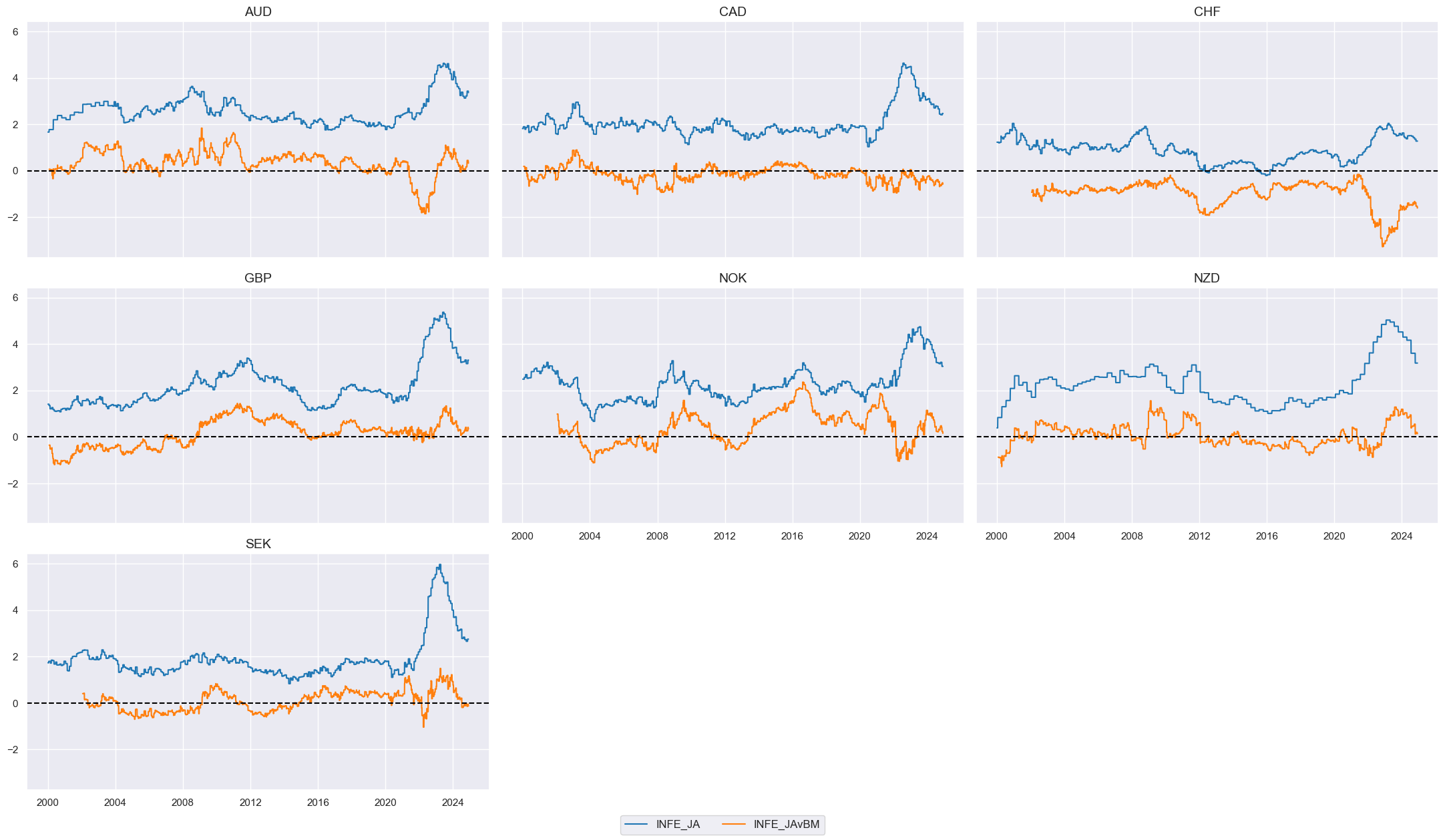
To display and compare the values for one of the resulting
INFE_JAvBM
indicator we use
view_timelines()
function from the
macrosynergy
package:
# Check time series
xc = "INFE_JA"

cidx = cids_dmfx
xcatx = [xc, xc + "vBM"]

msp.view_timelines(
    df=dfx,
    xcats=xcatx,
    cids=cidx,
    start="2000-01-01",
    aspect=1.7,
    ncol=3,
)
The negatives of relative unemployment rates and international liabilities to GDP series are defined. This is done for convenience, all constituent candidates are given the “right sign” that makes their theoretically expected predictive direction positive.
# Negative values

xcatx = ["UNEMPLRATE_SA_DvBM", "IIPLIABGDP_NSA_D"]
calcs = []

for xc in xcatx:
    calcs += [f"{xc}_NEG = - {xc}"]

dfa = msp.panel_calculator(dfx, calcs=calcs, cids=cids_dmfx)
dfx = msm.update_df(dfx, dfa)
# Conceptual features with theoretical positive FX impact

cpos = [
    "INFE_JAvBM",
    "CTOT_NSA_PAR",
    "UNEMPLRATE_SA_DvBM_NEG",
    "IIPLIABGDP_NSA_D_NEG",
    "RIR_NSAvBM",
    "XCPIXFE_SA_PARvBM",
    "MBCSCORE_SA_D",
    "XPGDPTECH_SA_P1M1ML12_3MMAvBM",
    "INTRGDP_NSA_P1M1ML12_3MMAvBM",
]
cpos.sort()
We normalize the plausible indicators collected in the list
cpos
above using
make_zn_scores()
function. This is a standard procedure aimed at making various categories comparable, in particular, summing or averaging categories with different units and time series properties.
# Zn-scores

xcatx = cpos
cidx = cids_dmfx

dfa = pd.DataFrame(columns=list(dfx.columns))

for xc in xcatx:
    dfaa = msp.make_zn_scores(
        dfx,
        xcat=xc,
        cids=cidx,
        sequential=True,
        min_obs=261 * 3,
        neutral="zero",
        pan_weight=1,
        thresh=4,
        postfix="_ZN",
        est_freq="m",
    )
    dfa = msm.update_df(dfa, dfaa)

dfx = msm.update_df(dfx, dfa)
cpoz = [x + "_ZN" for x in cpos]
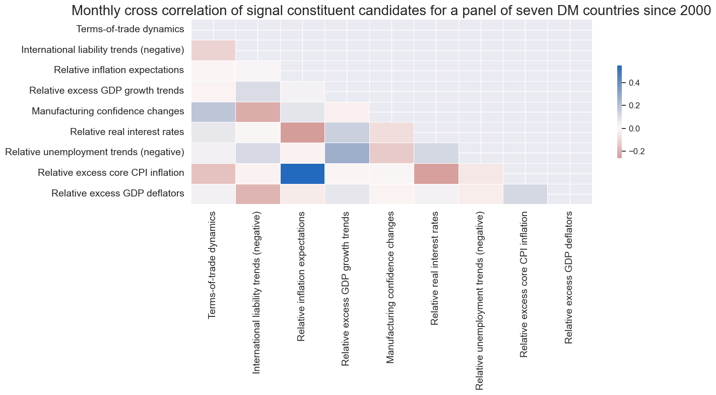
Renaming indicators to more intuitive names rather than technical tickers is a beneficial practice for enhancing the readability and interpretability of data analyses.
The
correl_matrix()
function visualizes correlation coefficient between signal constituent candidates for a panel of seven DM countries since
cidx = cids_dmfx
xcatx = cpoz

sdate = "2000-01-01"

renaming_dict = {
    "CTOT_NSA_PAR_ZN": "Terms-of-trade dynamics",
    "IIPLIABGDP_NSA_D_NEG_ZN": "International liability trends (negative)",
    "INFE_JAvBM_ZN": "Relative inflation expectations",
    "INTRGDP_NSA_P1M1ML12_3MMAvBM_ZN": "Relative excess GDP growth trends",
    "MBCSCORE_SA_D_ZN": "Manufacturing confidence changes",
    "RIR_NSAvBM_ZN": "Relative real interest rates",
    "UNEMPLRATE_SA_DvBM_NEG_ZN": "Relative unemployment trends (negative)",
    "XCPIXFE_SA_PARvBM_ZN": "Relative excess core CPI inflation",
    "XPGDPTECH_SA_P1M1ML12_3MMAvBM_ZN": "Relative excess GDP deflators",
}

dfx_corr = dfx.copy()

for key, value in renaming_dict.items():
    dfx_corr["xcat"] = dfx_corr["xcat"].str.replace(key, value)

msp.correl_matrix(
    dfx_corr,
    xcats=list(renaming_dict.values()),
    cids=cidx,
    start=sdate,
    freq="M",
    cluster=False,
    title="Monthly cross correlation of signal constituent candidates for a panel of seven DM countries since 2000",
    size=(14, 8),
)
Signal preparations #
Conceptual parity as benchmark #
linear_composite
method from the
macrosynergy
package aggregates the individual category scores into a unified (equally weighted) composite indicator
ALL_AVGZ
.
ALL_AVGZ
composite indicator serves as a benchmark for subsequent analyses, particularly in comparing its performance or relevance against signals optimized through machine learning techniques. By doing so, this composite indicator becomes a standard reference point, enabling a systematic evaluation of the effectiveness of machine learning-derived signals in capturing the underlying dynamics represented by the individual category scores.
# Linear equally-weighted combination of all available candidates

xcatx = cpoz
cidx = cids_dmfx

dfa = msp.linear_composite(
    df=dfx,
    xcats=cpoz,
    cids=cidx,
    new_xcat="ALL_AVGZ",
)
dfx = msm.update_df(dfx, dfa)
Convert data to scikit-learn format #
Downsampling daily information states to a monthly frequency is a common preparation step for machine learning models, especially when dealing with financial and economic time series data. The
categories_df()
function applies the leg of 1 month and uses the last value in the month for explanatory variables and the sum for the aggregated target (return). As explanatory variables, we use plausible z-scores of economic variables derived earlier and collected in the list
cpos
. As a target, we use
FXXR_VT10
, FX forward return for 10% vol target: dominant cross.
cidx = cids_dmfx
xcatx = cpoz + ["FXXR_VT10"]

# Downsample from daily to monthly frequency (features as last and target as sum)
dfw = msm.categories_df(
    df=dfx,
    xcats=xcatx,
    cids=cidx,
    freq="M",
    lag=1,
    blacklist=fxblack,
    xcat_aggs=["last", "sum"],
)

# Drop rows with missing values and assign features and target
dfw.dropna(inplace=True)
X_fx = dfw.iloc[:, :-1]
y_fx = dfw.iloc[:, -1]
Define splitter and scorer #
The
RollingKFoldPanelSplit
class instantiates splitters where temporally adjacent panel training sets of fixed joint maximum time spans can border the test set from both the past and future. Thus, most folds do not respect the chronological order but allow training with past and future information. While this does not simulate the evolution of information, it makes better use of the available data and is often acceptable for macro data as economic regimes come in cycles. It is equivalent to
scikit-learn
’s
Kfold class
but adapted for panels.
The standard
make_scorer()
function from the
scikit-learn
library is used to create a scorer object that is used to evaluate the performance on the test set. The standard
r2_score
function is used as a scorer.
splitter = msl.RollingKFoldPanelSplit(n_splits=5)
scorer = make_scorer(r2_score, greater_is_better=True)
The method
visualise_splits()
is a convenient method for visualizing the splits produced by each child splitter, giving the user confidence in the splits produced for their use case.
splitter.visualise_splits(X_fx, y_fx)

OLS/NNLS regression-based learning #
Sequential optimization and analysis #
For a straightforward Ordinary Least Squares (OLS) learning process, employing the
LinearRegression()
from
scikit-learn
offers a streamlined and efficient approach to regression analysis. When setting up this model for machine learning, two hyperparameter decisions can significantly influence the model’s behavior and its interpretation of the data:
-
Non-negativity constraint: This offers the option of non-negative least squares (NNLS), rather than simple OLS. NNLS imposes the constraint that the coefficients must be non-negative. The benefit of this restriction is that it allows consideration of theoretical priors on the direction of impact, reducing dependence on scarce data.
-
Inclusion of a regression intercept: Conceptually the neutral level of all (mostly relative) signal constituent candidates is zero. Hence, the regression intercept is presumed to be zero, albeit that may not always be exact, and some theoretical assumptions may have been wrong.
# Specify model options and grids

mods_ols = {
    "ls": LinearRegression(),
}

grid_ols = {
    "ls": {"positive": [True, False], "fit_intercept": [True, False]},
}
SignalOptimizer
class from the
macrosynergy
package is a sophisticated tool designed to facilitate the process of optimizing and evaluating different signals (predictors) for forecasting models in a time series context. Leveraging the earlier defined cross-validation split (
RollingKFoldPanelSplit
), the blacklist period, defined data frames of dependent and independent variables, and a few other optional parameters, we instantiate the
SignalOptimizer
class.
calculate_predictions()
method is used to calculate, store and return sequentially optimized signals for a given process. This method implements the nested cross-validation and subsequent signal generation. The name of the process, together with models to fit, hyperparameters to search over and a metric to optimize, are provided as compulsory arguments.
xcatx = cpoz + ["FXXR_VT10"]
cidx = cids_dmfx

so_ls = msl.SignalOptimizer(
    df = dfx,
    xcats = xcatx,
    cids = cidx,
    blacklist = fxblack,
    freq = "M",
    lag = 1,
    xcat_aggs = ["last", "sum"]
)
so_ls.calculate_predictions(
    name = "LS",
    models = mods_ols,
    hyperparameters = grid_ols,
    scorers = {"r2": scorer},
    inner_splitters = {"Rolling": splitter},
    search_type = "grid",
    normalize_fold_results = False,
    cv_summary = "mean",
    min_cids = 2,
    min_periods = 36,
    test_size = 1,
    n_jobs_outer = -1,
    split_functions={"Rolling": lambda n: n // 36},
)

dfa = so_ls.get_optimized_signals()
dfx = msm.update_df(dfx, dfa)
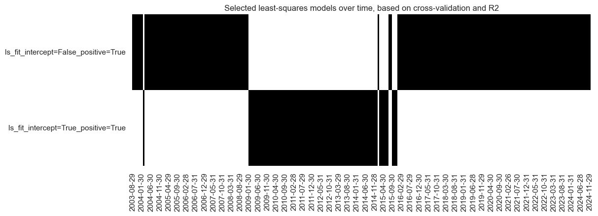
The “heatmap” serves as a powerful tool to illustrate the evolution and selection of predictive models over time, especially in a context. When the visualization indicates that over time the preferred model becomes the most restrictive one, it suggests a shift towards models with tighter constraints or fewer degrees of freedom.
so_ls.models_heatmap(
    name="LS",
    cap=6,
    title="Selected least-squares models over time, based on cross-validation and R2",
    figsize=(12, 4),
)
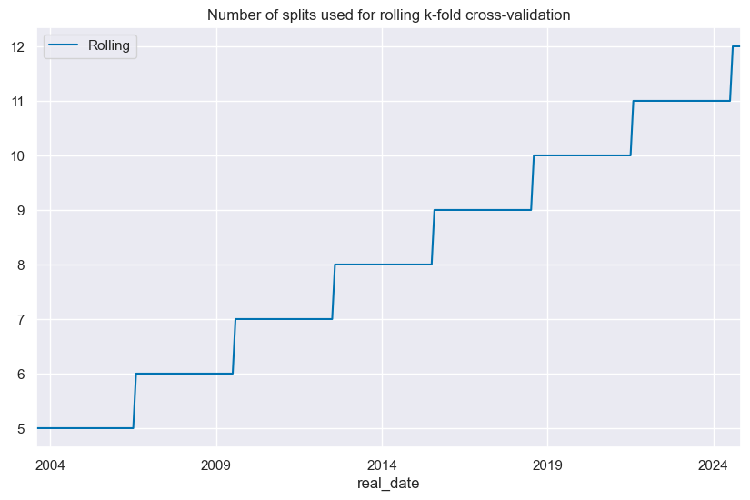
# Number of splits used for cross-validation over time

so_ls.nsplits_timeplot("LS", title="Number of splits used for rolling k-fold cross-validation")
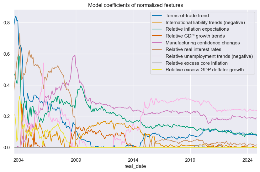
The
feature_importance_timeplot()
method is designed for plotting the time series of feature coefficients obtained from regression models over time. This kind of visualization can be particularly valuable to understand the dynamics and stability of model coefficients, which is crucial for interpretation and forecasting.
ftrs_dict = {
    "CTOT_NSA_PAR_ZN": "Terms-of-trade trend",
    "IIPLIABGDP_NSA_D_NEG_ZN": "International liability trends (negative)",
    "INFE_JAvBM_ZN": "Relative inflation expectations",
    "INTRGDP_NSA_P1M1ML12_3MMAvBM_ZN": "Relative GDP growth trends",
    "MBCSCORE_SA_D_ZN": "Manufacturing confidence changes",
    "RIR_NSAvBM_ZN": "Relative real interest rates",
    "UNEMPLRATE_SA_DvBM_NEG_ZN": "Relative unemployment trends (negative)",
    "XCPIXFE_SA_PARvBM_ZN": "Relative excess core inflation",
    "XPGDPTECH_SA_P1M1ML12_3MMAvBM_ZN": "Relative excess GDP deflator growth",
}

so_ls.feature_importance_timeplot("LS", title="Model coefficients of normalized features",ftrs_renamed=ftrs_dict)
coefs_stackedbarplot()
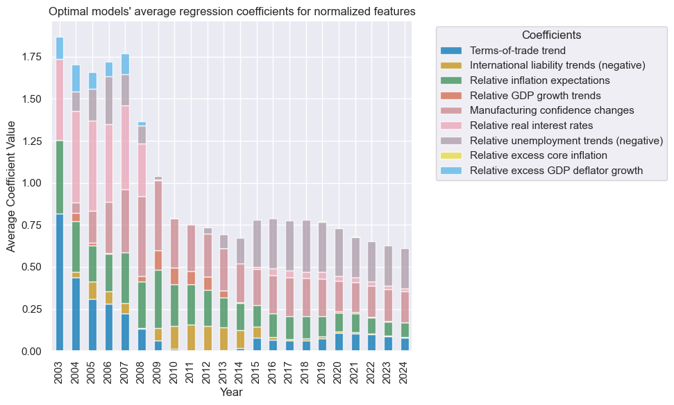
is another convenient function, generating stacked bar plots to visualize the coefficients of features from regression models. This visualization method effectively displays the magnitude and direction of each feature’s influence on the outcome, allowing for easy comparison and interpretation of how different predictors contribute to the model.
so_ls.coefs_stackedbarplot("LS",
                           title="Optimal models' average regression coefficients for normalized features",
                           ftrs_renamed=ftrs_dict)
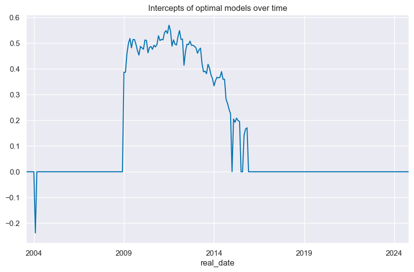
The
intercepts_timeplot()
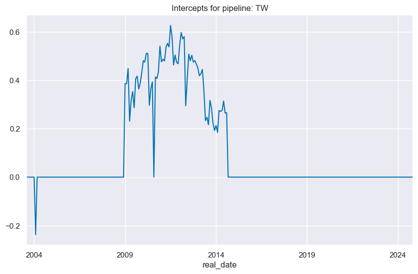
function is designed to plot the time series of intercepts from regression models, enabling an analysis of how the model intercepts change over time.
so_ls.intercepts_timeplot("LS",
                          title="Intercepts of optimal models over time")
To display and compare the values for conceptual parity
ALL_AVGZ
versus OLS-based learning indicator
LS
we use
view_timelines()
function from the
macrosynergy
package
sigs_ls = [
    "ALL_AVGZ",
    "LS",
]
xcatx = sigs_ls
cidx = cids_dmfx

msp.view_timelines(
    dfx,
    xcats=xcatx,
    cids=cidx,
    ncol=4,
    start="2003-08-29",
    title="Developed market FX forward trading signals: conceptual parity versus OLS-based learning",
    title_fontsize=30,
    same_y=False,
    cs_mean=False,
    xcat_labels=["Conceptual parity signal", "OLS-based learning signal"],
    legend_fontsize=16,
)

Signal value checks #
Specs and panel test #
sigs = ["ALL_AVGZ", "LS"]
targs = ["FXXR_VT10"]
cidx = cids_dmfx
sdate = "2003-08-29"

dict_ls = {
    "sigs": sigs,
    "targs": targs,
    "cidx": cidx,
    "start": sdate,
    "black": fxblack,
    "srr": None,
    "pnls": None,
}
CategoryRelations
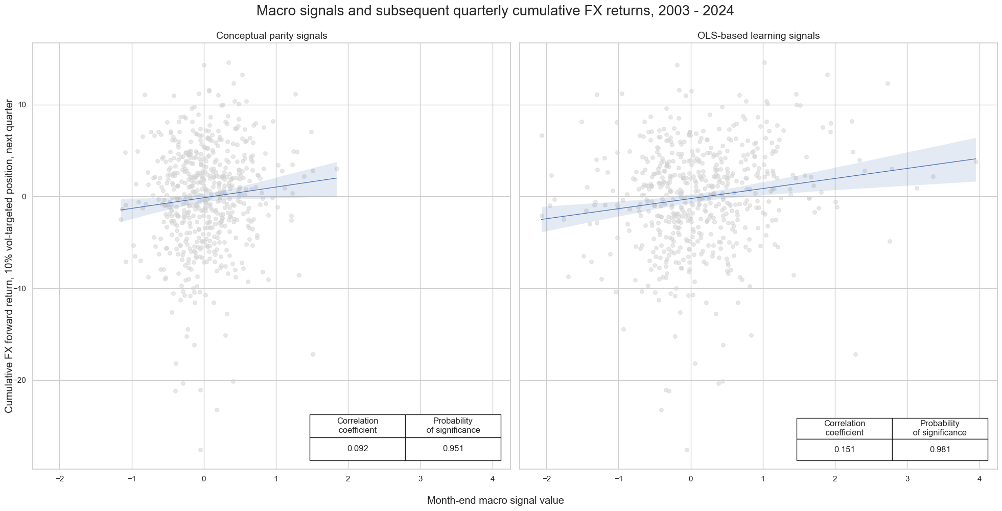
facilitates the visualization and analysis of relationships between two specific categories, namely, two panels of time series data. This tool is used to examine the interaction between the risk parity “ALL_AVGZ”, and optimized “LS” - on one side, and the FXXR_VT10, which represents the FX forward return for a 10% volatility target, focusing on the dominant cross, on the other. The
multiple_reg_scatter
method of the class displays correlation scatters for the two pairs.
The plot below shows the significant positive predictive power of the OLS learning-based signals with respect to subsequent weekly, monthly, and quarterly FX returns. The correlation coefficient for the OLS learning-based signal is considerably higher than for the risk parity version.
dix = dict_ls

sigx = dix["sigs"]
tarx = dix["targs"]
cidx = dix["cidx"]
blax = dix["black"]
start = dix["start"]

def crmaker(sig, targ):
    crx = msp.CategoryRelations(
        dfx,
        xcats=[sig, targ],
        cids=cidx,
        freq="Q",
        lag=1,
        xcat_aggs=["last", "sum"],
        start=start,
        blacklist=blax,
    )
    return crx


lcrs = [crmaker(sig, targ) for sig in sigx for targ in tarx]

msv.multiple_reg_scatter(
    lcrs,
    ncol=2,
    nrow=1,
    figsize=(20, 10),
    title="Macro signals and subsequent quarterly cumulative FX returns, 2003 - 2024",
    xlab="Month-end macro signal value",
    ylab="Cumulative FX forward return, 10% vol-targeted position, next quarter",
    coef_box="lower right",
    prob_est="map",
    subplot_titles=["Conceptual parity signals", "OLS-based learning signals"],
)
Accuracy and correlation check #
The
SignalReturnRelations
class of the
macrosynergy
package is specifically designed to assess the predictive power of signal categories in determining the direction of subsequent returns, particularly for data structured in the JPMaQS format. This class provides a streamlined approach for evaluating how well a given signal can forecast future market movements, offering insights for investment strategies, risk management, and economic analysis. It helps to identify which indicators have more predictive power.
## Compare optimized signals with simple average z-scores

dix = dict_ls

sigx = dix["sigs"]
tarx = dix["targs"]
cidx = dix["cidx"]
blax = dix["black"]
startx = dix["start"]

srr = mss.SignalReturnRelations(
    df=dfx,
    rets=tarx,
    sigs=sigx,
    cids=cidx,
    cosp=True,
    freqs=["M"],
    agg_sigs=["last"],
    start=startx,
    blacklist=blax,
    slip=1,
    ms_panel_test=True,
)
dix["srr"] = srr
srr = dict_ls["srr"]

selcols = [
    "accuracy",
    "bal_accuracy",
    "pos_sigr",
    "pos_retr",
    "pearson",
    "map_pval",
    "kendall",
    "kendall_pval",
]
srr.multiple_relations_table().round(3)[selcols]
| accuracy | bal_accuracy | pos_sigr | pos_retr | pearson | map_pval | kendall | kendall_pval | ||||
|---|---|---|---|---|---|---|---|---|---|---|---|
| Return | Signal | Frequency | Aggregation | ||||||||
| FXXR_VT10 | ALL_AVGZ | M | last | 0.526 | 0.526 | 0.495 | 0.505 | 0.057 | 0.027 | 0.044 | 0.006 |
| LS | M | last | 0.535 | 0.535 | 0.530 | 0.505 | 0.095 | 0.016 | 0.070 | 0.000 |
Naive PnL #
In this analysis, the notebook calculates the naive Profit and Loss (PnL) for foreign exchange (FX) strategies utilizing both risk parity and OLS-based learning indicators. These PnL calculations are derived from simple trading strategies that interpret the indicators as signals to either go long (buy) or short (sell) FX positions. Specifically, the direction of the indicators guides the trading decisions, where a positive signal might suggest buying (going long) the FX asset, and a negative signal might suggest selling (going short). This approach allows for a direct evaluation of how effectively each indicator—risk parity and OLS-based—can predict profitable trading opportunities in the FX market.
Please refer to
                NaivePnl()


                class
for details.
dix = dict_ls

sigx = dix["sigs"]
tarx = dix["targs"]
cidx = dix["cidx"]
blax = dix["black"]
startx = dix["start"]

pnls = msn.NaivePnL(
    df=dfx,
    ret=tarx[0],
    sigs=sigx,
    cids=cidx,
    start=startx,
    blacklist=blax,
    bms=["USD_GB10YXR_NSA", "EUR_FXXR_NSA", "USD_EQXR_NSA"],
)
for sig in sigx:
    pnls.make_pnl(
        sig=sig,
        sig_op="zn_score_pan",
        rebal_freq="monthly",
        neutral="zero",
        rebal_slip=1,
        vol_scale=10,
        thresh=4,
    )
pnls.make_long_pnl(vol_scale=10, label="Long only")

dix["pnls"] = pnls
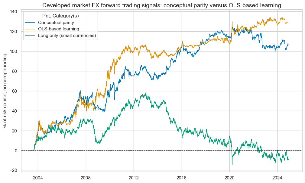
The PnLs are plotted using
.plot_pnls()
method of the
NaivePnl()
class
. The performance characteristics of the learning-based signal are encouraging. One should consider that the strategy only has seven markets to trade in, some of which are highly correlated. Also, the strategy only macro signals, without any other consideration of market prices and volumes. Position changes are infrequent and gentle.
pnls = dix["pnls"]
sigx = dix["sigs"]

pnls.plot_pnls(
    title="Developed market FX forward trading signals: conceptual parity versus OLS-based learning",
    title_fontsize=14,
    xcat_labels=["Conceptual parity", "OLS-based learning", "Long only (small currencies)"],
)
pnls.evaluate_pnls(pnl_cats=["PNL_" + sig for sig in sigx] + ["Long only"])
| xcat | PNL_ALL_AVGZ | PNL_LS | Long only |
|---|---|---|---|
| Return % | 5.049094 | 6.054965 | -0.433958 |
| St. Dev. % | 10.0 | 10.0 | 10.0 |
| Sharpe Ratio | 0.504909 | 0.605497 | -0.043396 |
| Sortino Ratio | 0.711546 | 0.85664 | -0.059703 |
| Max 21-Day Draw % | -17.7254 | -15.013328 | -23.133937 |
| Max 6-Month Draw % | -14.745215 | -14.601964 | -22.868546 |
| Peak to Trough Draw % | -30.190283 | -17.516423 | -72.266181 |
| Top 5% Monthly PnL Share | 0.741356 | 0.577154 | -8.061563 |
| USD_GB10YXR_NSA correl | -0.088757 | -0.072222 | -0.012885 |
| EUR_FXXR_NSA correl | 0.13088 | 0.140748 | 0.409875 |
| USD_EQXR_NSA correl | 0.120495 | 0.032309 | 0.245412 |
| Traded Months | 257 | 257 | 257 |
Alternative models of regression-based learning #
Regularized linear model (elastic net) #
Beyond simple OLS regression-based learning the post considers three other types of regression-based learning processes.
The first alternative model is Regularized regression-based learning ElasticNet
# Specify model options and grids

mods_en = {
    "en": ElasticNet(),
    "ls": LinearRegression(),
}

grid_en = {
    "en": {
        "positive": [True, False],
        "fit_intercept": [True, False],
        "alpha": [1e-4, 1e-3, 1e-2, 1e-1, 1],
        "l1_ratio": [0.1, 0.25, 0.5, 0.75, 0.9]
    },
    "ls": {
        "positive": [True, False],
        "fit_intercept": [True, False],
    }
}
For the ElasticNet model, similar to the OLS regression approach,
SignalOptimizer
class from the
macrosynergy
package is instantiated using earlier defined cross-validation split (
RollingKFoldPanelSplit
), blacklist period, dataframes of dependent and independent variables and a few other optional parameters.
calculate_predictions()
method is used to calculate, store and return sequentially optimized signals for a given process. This method implements the nested cross-validation and subsequent signal generation. The name of the process, together with models to fit, hyperparameters to search over and a metric to optimize, are provided as compulsory arguments.
xcatx = cpoz + ["FXXR_VT10"]
cidx = cids_dmfx

so_en = msl.SignalOptimizer(
    df = dfx,
    xcats = xcatx,
    cids = cidx,
    blacklist = fxblack,
    freq = "M",
    lag = 1,
    xcat_aggs = ["last", "sum"]
)
so_en.calculate_predictions(
    name = "EN",
    models = mods_en,
    hyperparameters = grid_en,
    scorers = {"r2": scorer},
    inner_splitters = {"Rolling": splitter},
    search_type = "grid",
    normalize_fold_results = False,
    cv_summary = "mean",
    min_cids = 2,
    min_periods = 36,
    test_size = 1,
    n_jobs_outer = -1,
    split_functions={"Rolling": lambda n: n // 36},
)

dfa = so_en.get_optimized_signals()
dfx = msm.update_df(dfx, dfa)
The “heatmap” serves as a powerful tool to illustrate the evolution and selection of predictive models over time.
# Illustrate model choice

so_en.models_heatmap(
    "EN",
    title="Selected elastic net models over time, based on cross-validation and R2",
    figsize=(12, 3),
)

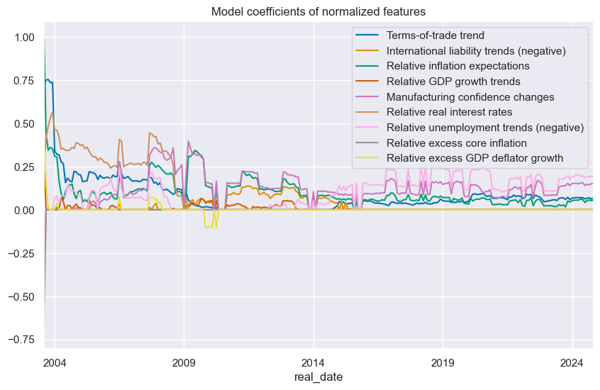
The
feature_importance_timeplot()
function is used to plot the time series of feature coefficients, providing a visual representation of how the importance or influence of each feature in the model changes over time.
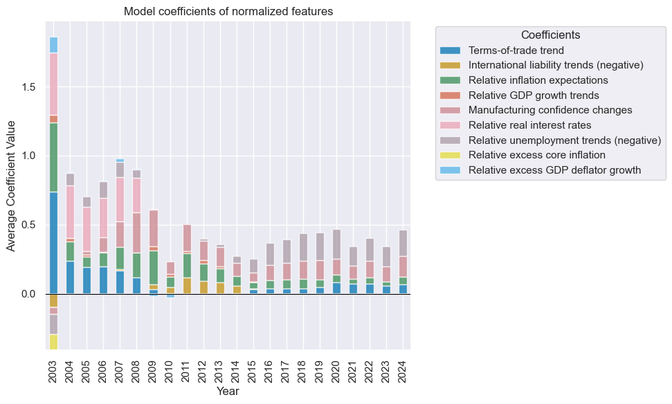
so_en.feature_importance_timeplot("EN", title="Model coefficients of normalized features", ftrs_renamed=ftrs_dict)
coefs_stackedbarplot()
is another convenient function, allowing to create a stacked bar plot of feature coefficients.
so_en.coefs_stackedbarplot("EN", title="Model coefficients of normalized features", ftrs_renamed=ftrs_dict)
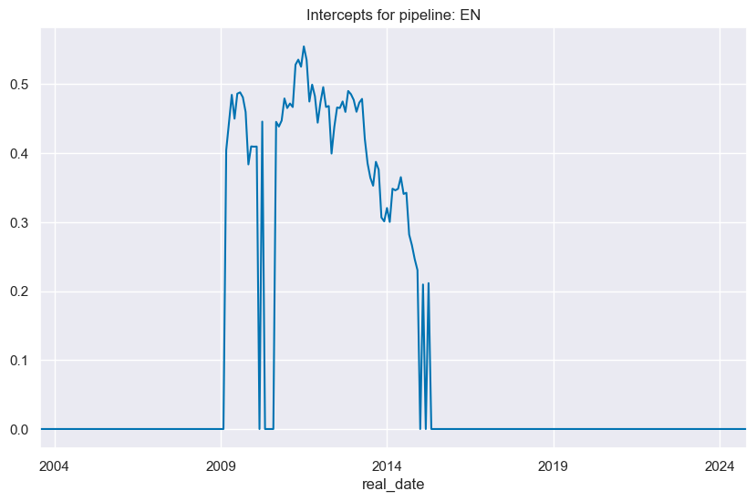
intercepts_timeplot()
plots the time series of intercepts.
so_en.intercepts_timeplot("EN")
Sign-weighted linear regression #
The second alternative machine learning model is sign-weighted WLS linear regression. Sign-weighted least squares equalize the contribution of positive and negative target samples to the model fit. The learning process can choose between sign-weighted and ordinary least squares, both with intercept exclusion and non-negativity constraints.
SignWeightedLinearRegression
is a custom class to create a WLS linear regression model, with the sample weights chosen by inverse frequency of the label’s sign in the training set.
As for simple OLS regression, two hyperparameter decisions need to be made:
-
Non-negativity constraint: This offers the option of non-negative least squares (NNLS), rather than simple OLS. NNLS imposes the constraint that the coefficients must be non-negative. The benefit of this restriction is that it allows for the consideration of theoretical priors on the direction of impact, reducing dependence on scarce data.
-
Inclusion of a regression intercept: Conceptually the neutral level of all (mostly relative) signal constituent candidates is zero. Hence, the regression intercept is presumed to be zero, albeit that may not always be exact, and some theoretical assumptions may have been wrong.
# Specify model options and grids

mods_sw = {
    "swls": msl.SignWeightedLinearRegression(),
    "ls": LinearRegression(),
}

grid_sw = {
    "swls": {"positive": [True, False], "fit_intercept": [True, False]},
    "ls": {"positive": [True, False], "fit_intercept": [True, False]},
}
SignalOptimizer
class from the
macrosynergy
package is instantiated using earlier defined cross-validation split (RollingKFoldPanelSplit), blacklist period, dataframes of dependent and independent variables and few other optional parameters.
calculate_predictions()
method is used to calculate, store and return sequentially optimized signals for a given process. This method implements the nested cross-validation and subsequent signal generation. The name of the process, together with models to fit, hyperparameters to search over and a metric to optimize, are provided as compulsory arguments.
xcatx = cpoz + ["FXXR_VT10"]
cidx = cids_dmfx

so_sw = msl.SignalOptimizer(
    df = dfx,
    xcats = xcatx,
    cids = cidx,
    blacklist = fxblack,
    freq = "M",
    lag = 1,
    xcat_aggs = ["last", "sum"]
)
so_sw.calculate_predictions(
    name = "SW",
    models = mods_sw,
    hyperparameters = grid_sw,
    scorers = {"r2": scorer},
    inner_splitters = {"Rolling": splitter},
    search_type = "grid",
    normalize_fold_results = False,
    cv_summary = "mean",
    min_cids = 2,
    min_periods = 36,
    test_size = 1,
    n_jobs_outer = -1,
    split_functions={"Rolling": lambda n: n // 36},
)

dfa = so_sw.get_optimized_signals()
dfx = msm.update_df(dfx, dfa)
The “heatmap” serves as a powerful tool to illustrate the evolution and selection of predictive models over time:
# Illustrate model choice

so_sw.models_heatmap(
    "SW",
    title="Selected sign-weighted or unweighted least square models, based on cross-validation and R2",
    figsize=(12, 3),
)

Time-weighted regression #
The last alternative machine learning model is time-weighted regression-based learning. Time-Weighted Least Squares allow prioritizing more recent information in the model fit by defining a half-life of exponential decay in units of the native dataset frequency. The learning process can choose between time-weighted and ordinary least squares.
TimeWeightedLinearRegression
is a custom class to create a WLS linear regression model, where the training sample weights exponentially decay by sample recency, given a prescribed half_life.
Key hyperparameters of this model are:
-
Non-negativity constraint: option of non-negative least squares (NNLS), rather than simple OLS
-
Inclusion of a regression intercept: decides whether to include an intercept, acknowledging cases where the assumption of a zero neutral level might not hold.
-
Half-life specification: defines the decay rate for weighting recent observations more heavily, with a selectable range between 12 to 240 months, adapting the model to the specific temporal sensitivity of the dataset.
# Specify model options and grids

mods_tw = {
    "twls": msl.TimeWeightedLinearRegression(),
    "ls": LinearRegression(),
}

grid_tw = {
    "twls": {"positive": [True, False], "fit_intercept": [True, False], "half_life": [12, 24, 36, 60, 120, 240]},
    "ls": {"positive": [True, False], "fit_intercept": [True, False]},
}
SignalOptimizer
class from the
macrosynergy
package is instantiated using a time-respecting cross-validator split (
ExpandingKFoldPanelSplit
), blacklist period, dataframes of dependent and independent variables and few other optional parameters. This expanding splitter is required because the model takes into account the sequential component of the panel.
calculate_predictions()
method is used to calculate, store and return sequentially optimized signals for a given process. This method implements the nested cross-validation and subsequent signal generation. The name of the process, together with models to fit, hyperparameters to search over and a metric to optimize, are provided as compulsory arguments.
xcatx = cpoz + ["FXXR_VT10"]
cidx = cids_dmfx

so_tw = msl.SignalOptimizer(
    df = dfx,
    xcats = xcatx,
    cids = cidx,
    blacklist = fxblack,
    freq = "M",
    lag = 1,
    xcat_aggs = ["last", "sum"]
)
so_tw.calculate_predictions(
    name = "TW",
    models = mods_tw,
    hyperparameters = grid_tw,
    scorers = {"r2": scorer},
    inner_splitters = {"Rolling": splitter},
    search_type = "grid",
    normalize_fold_results = False,
    cv_summary = "mean",
    min_cids = 2,
    min_periods = 36,
    test_size = 1,
    n_jobs_outer = -1,
    split_functions={"Rolling": lambda n: n // 36},
)

dfa = so_tw.get_optimized_signals()
dfx = msm.update_df(dfx, dfa)
The “heatmap” serves as a powerful tool to illustrate the evolution and selection of predictive models over time
# Illustrate model choice

so_tw.models_heatmap(
    "TW",
    title="Selected time-weighted or unweighted least square models, based on cross-validation and R2",
    figsize=(12, 3),
)

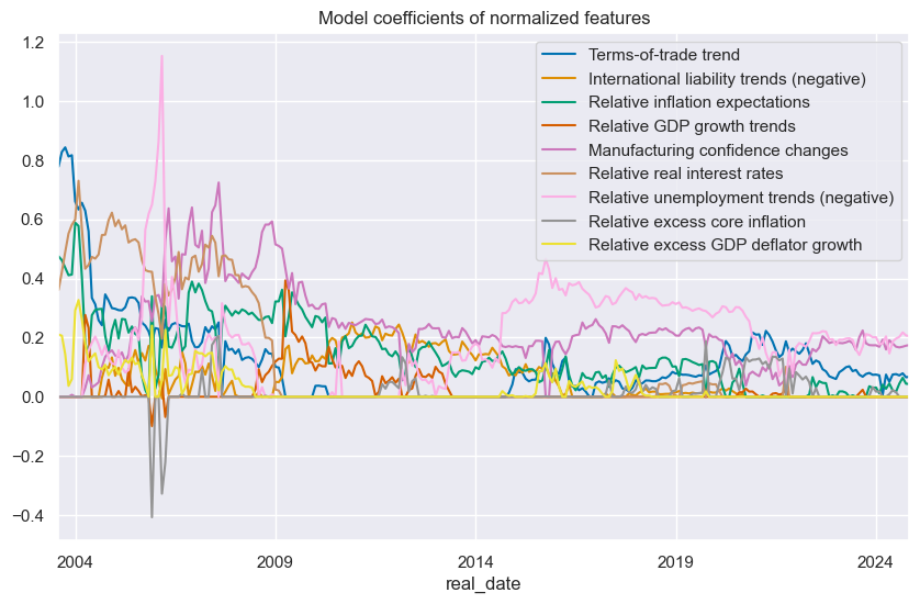
so_tw.feature_importance_timeplot("TW", title="Model coefficients of normalized features", ftrs_renamed=ftrs_dict)
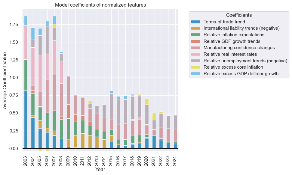
so_tw.coefs_stackedbarplot("TW", title="Model coefficients of normalized features", ftrs_renamed=ftrs_dict)
so_tw.intercepts_timeplot("TW")
Signal value checks #
Specs and panel test #
This part of the notebook checks and compares the predictive powers of the three alternative regression-based learning processes:
• Regularized regression-based learning
• Sign-weighted regression-based learning
• Time-weighted regression-based learning
with standard regression-based learning approach OLS.
This part follows the same structure as above, where we compared conceptual parity
ALL_AVGZ
versus OLS-based learning indicator
LS
. In this part, we compare the four optimized indicators generated by the above models:
-
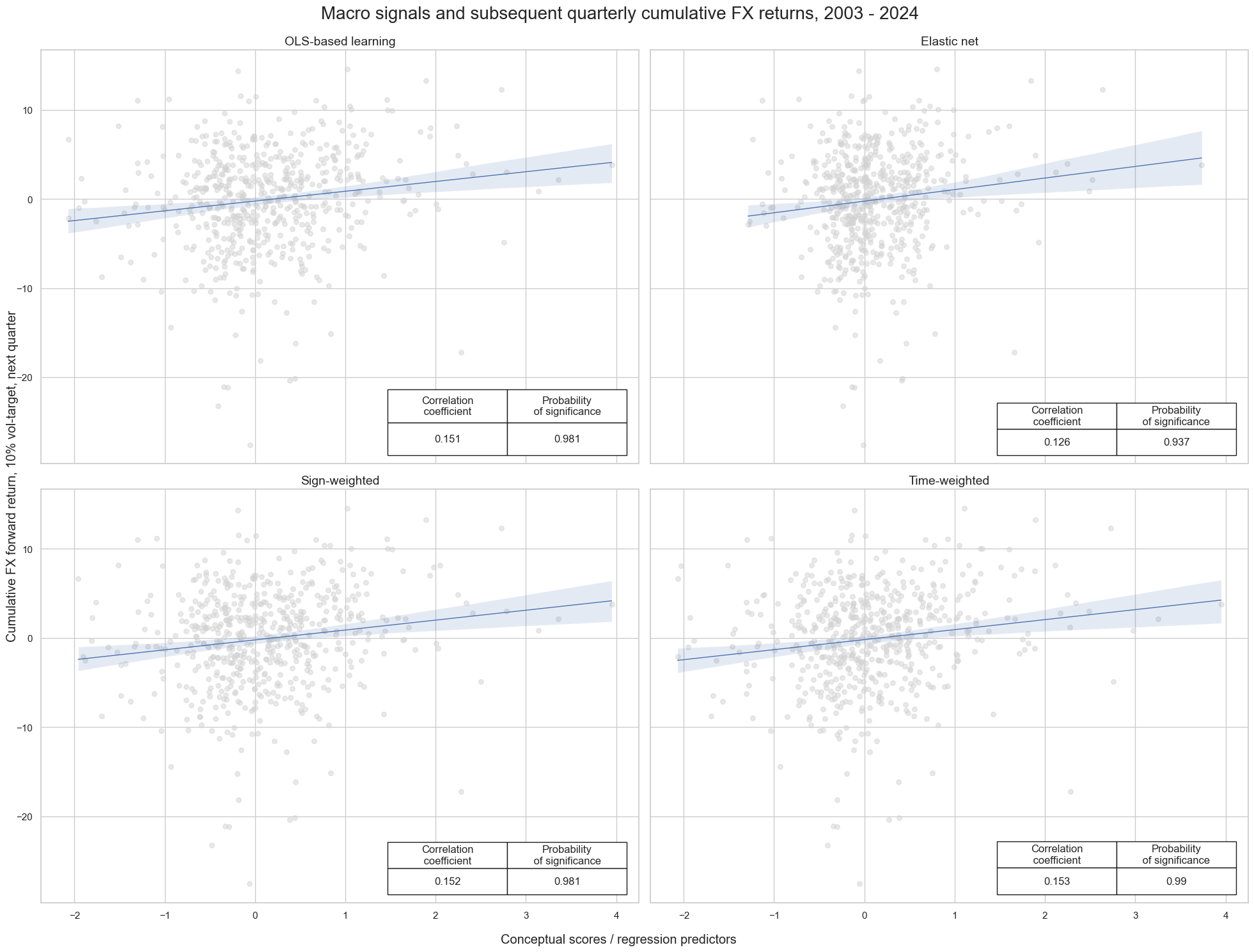
CategoryRelationsandmultiple_reg_scatteranalyze and visualize the relationships between the four optimized signals - “LS”, “EN”, “SW”, “TW” - on one side, and the FXXR_VT10, which represents the FX forward return for a 10% volatility target, focusing on the dominant cross, on the other. -
The
SignalReturnRelationsclass of themacrosynergypackage assess the predictive power of the signals -
                  NaivePnl()


                  class
provides a quick and simple overview of a stylized PnL profile of a set of trading signals and plots line charts of cumulative PnLs:
sigs = ["ALL_AVGZ", "LS", "EN", "SW", "TW"]
targs = ["FXXR_VT10"]
cidx = cids_dmfx

dict_ams = {
    "sigs": sigs,
    "targs": targs,
    "cidx": cidx,
    "start": dix["start"],
    "black": fxblack,
    "srr": None,
    "pnls": None,
}
dix = dict_ams

sigx = dix["sigs"]
tarx = dix["targs"]
cidx = dix["cidx"]
blax = dix["black"]
start = dix["start"]


def crmaker(sig, targ):
    crx = msp.CategoryRelations(
        dfx,
        xcats=[sig, targ],
        cids=cidx,
        freq="Q",
        lag=1,
        xcat_aggs=["last", "sum"],
        start=start,
        blacklist=blax,
    )
    return crx


lcrs = [crmaker(sig, targ) for sig in sigx[1:] for targ in tarx]

msv.multiple_reg_scatter(
    lcrs,
    ncol=2,
    nrow=2,
    title="Macro signals and subsequent quarterly cumulative FX returns, 2003 - 2024",
    xlab="Conceptual scores / regression predictors ",
    ylab="Cumulative FX forward return, 10% vol-target, next quarter",
    coef_box="lower right",
    prob_est="map",
    subplot_titles=["OLS-based learning", "Elastic net", "Sign-weighted", "Time-weighted"],
)
Accuracy and correlation check #
The
SignalReturnRelations
class of the
macrosynergy
package facilitates a quick assessment of the power of a signal category in predicting the direction of subsequent returns for data in JPMaQS format.
## Compare optimized signals

dix = dict_ams

sigx = dix["sigs"]
tarx = dix["targs"]
cidx = dix["cidx"]
blax = dix["black"]
start = dix["start"]

srr = mss.SignalReturnRelations(
    df=dfx,
    rets=tarx,
    sigs=sigx,
    cids=cids_dmfx,
    cosp=True,
    freqs=["M"],
    agg_sigs=["last"],
    start=start,
    blacklist=fxblack,
    slip=1,
    ms_panel_test=True,
)
dix["srr"] = srr
srr = dict_ams["srr"]

selcols = [
    "accuracy",
    "bal_accuracy",
    "pos_sigr",
    "pos_retr",
    "pearson",
    "map_pval",
    "kendall",
    "kendall_pval",
]
srr.multiple_relations_table().round(3)[selcols]
| accuracy | bal_accuracy | pos_sigr | pos_retr | pearson | map_pval | kendall | kendall_pval | ||||
|---|---|---|---|---|---|---|---|---|---|---|---|
| Return | Signal | Frequency | Aggregation | ||||||||
| FXXR_VT10 | ALL_AVGZ | M | last | 0.526 | 0.526 | 0.495 | 0.505 | 0.057 | 0.027 | 0.044 | 0.006 |
| EN | M | last | 0.537 | 0.537 | 0.548 | 0.504 | 0.076 | 0.095 | 0.056 | 0.000 | |
| LS | M | last | 0.535 | 0.535 | 0.530 | 0.505 | 0.095 | 0.016 | 0.070 | 0.000 | |
| SW | M | last | 0.541 | 0.541 | 0.520 | 0.505 | 0.093 | 0.022 | 0.068 | 0.000 | |
| TW | M | last | 0.535 | 0.535 | 0.511 | 0.505 | 0.083 | 0.025 | 0.062 | 0.000 |
Naive PnL #
NaivePnl()
class
from
macrosynergy
package is designed to provide a quick and simple overview of a stylized PnL profile of a set of trading signals.
The related
make_pnl()
method calculates and stores generic PnLs based on a range of signals and their transformations into positions. The positioning options include choice of trading frequency, z-scoring, simple equal-size long-short positions (-1/1) thresholds to prevent outsized positions, and rebalancing slippage.
The generated PnLs are, however, naive insofar as they do not consider trading costs and plausible risk management restrictions. Also, if a volatility scale is set this is done so ex-post, mainly for the benefit of plotting different signals’ PnLs in a single chart.
A complementary method is
make_long_pnl()
, which calculates a “long-only” PnL based on a uniform long position across all markets at all times. This often serves as a benchmark for gauging the benefits of active trading.
dix = dict_ams

sigx = dix["sigs"]
tarx = dix["targs"]
cidx = dix["cidx"]
blax = dix["black"]
start = dix["start"]

pnls = msn.NaivePnL(
    df=dfx,
    ret=tarx[0],
    sigs=sigx,
    cids=cidx,
    start=start,
    blacklist=fxblack,
    bms=["USD_GB10YXR_NSA", "EUR_FXXR_NSA", "USD_EQXR_NSA"],
)
for sig in sigx:
    pnls.make_pnl(
        sig=sig,
        sig_op="zn_score_pan",
        rebal_freq="monthly",
        neutral="zero",
        rebal_slip=1,
        vol_scale=10,
        thresh=3,
    )
pnls.make_long_pnl(vol_scale=10, label="Long only")

dix["pnls"] = pnls
The PnLs are plotted using
.plot_pnls()
method of the
NaivePnl()
class
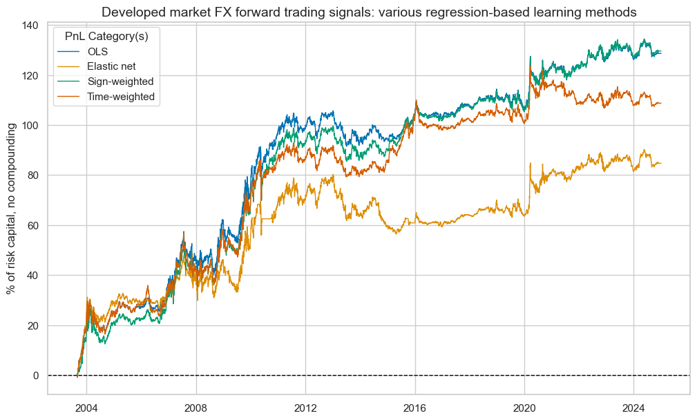
. These plots mainly inform on seasonality and stability of value generation under the assumption of negligible transaction costs. The post argues, that the underperformance of elastic net methods may not be accidental. Shrinkage-based regularization involves reducing model coefficients so that small changes in the input(s) lead to small changes in the predictions made. The idea is that introducing some bias into the regression can help reduce the variance in predictions made. Whilst theoretically sound, this in practice leads to more frequent model changes, as the appropriate type and size of penalties must be estimated based on the scarce data. This accentuates a source of signal variation that is unrelated to macro trends.
dix = dict_ams

pnls = dix["pnls"]
sigx = dix["sigs"]

pnls.plot_pnls(
    pnl_cats=["PNL_" + sig for sig in sigx[1:]],
    title="Developed market FX forward trading signals: various regression-based learning methods",
    title_fontsize=14,
    xcat_labels=["OLS", "Elastic net", "Sign-weighted", "Time-weighted"],
)
pnls.evaluate_pnls(pnl_cats=["PNL_" + sig for sig in sigx] + ["Long only"])
| xcat | PNL_ALL_AVGZ | PNL_LS | PNL_EN | PNL_SW | PNL_TW | Long only |
|---|---|---|---|---|---|---|
| Return % | 5.211949 | 6.029726 | 3.971191 | 6.072858 | 5.096418 | -0.433958 |
| St. Dev. % | 10.0 | 10.0 | 10.0 | 10.0 | 10.0 | 10.0 |
| Sharpe Ratio | 0.521195 | 0.602973 | 0.397119 | 0.607286 | 0.509642 | -0.043396 |
| Sortino Ratio | 0.735612 | 0.850947 | 0.555705 | 0.859513 | 0.715337 | -0.059703 |
| Max 21-Day Draw % | -14.843093 | -15.191913 | -12.361872 | -15.25575 | -15.228566 | -23.133937 |
| Max 6-Month Draw % | -14.105099 | -14.775656 | -17.854891 | -15.164625 | -18.310398 | -22.868546 |
| Peak to Trough Draw % | -30.795265 | -17.724782 | -23.882748 | -18.18197 | -21.200599 | -72.266181 |
| Top 5% Monthly PnL Share | 0.725327 | 0.579577 | 0.875488 | 0.572797 | 0.711704 | -8.061563 |
| USD_GB10YXR_NSA correl | -0.087311 | -0.071956 | -0.083888 | -0.071809 | -0.056761 | -0.012885 |
| EUR_FXXR_NSA correl | 0.124402 | 0.139716 | 0.17666 | 0.120693 | 0.12351 | 0.409875 |
| USD_EQXR_NSA correl | 0.118615 | 0.030918 | 0.039827 | 0.024582 | 0.01232 | 0.245412 |
| Traded Months | 257 | 257 | 257 | 257 | 257 | 257 |
Correcting linear models for statistical precision #
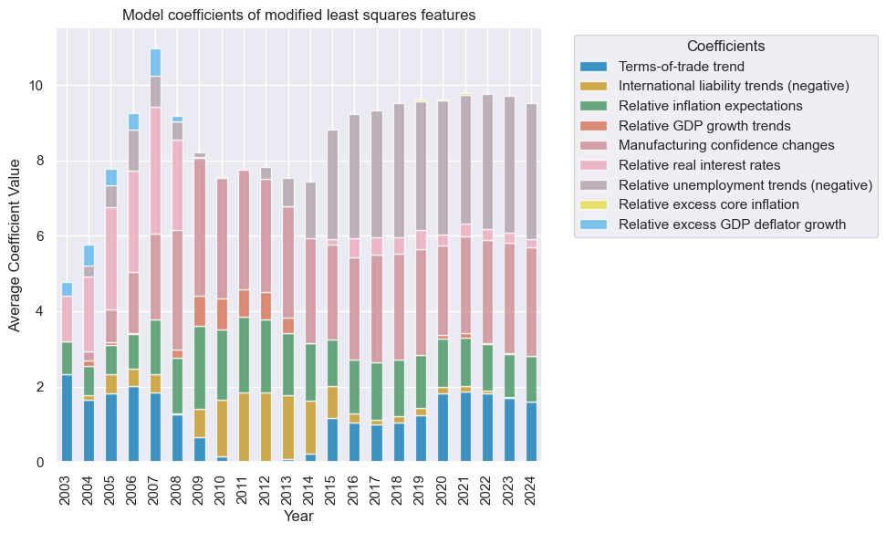
A notable issue with using regression-based learning as the sole component of a macro trading signal is that macroeconomic trends take time to form, meaning that model coefficients (and predictions) exhibit greater variability in early years, before the correlations have stabilised. As a consequence, absolute model coefficients have a tendency to decrease over time, producing smaller signals. This is exaggerated by the
NaivePnL
calculation because the signal considered by the PnL is a windorized z-score with standard deviation updated over time.
One way of mitigating this is by adjusting linear model coefficients by their estimated standard errors. The resulting factor model has coefficients that take into account statistical precision of the parameter estimates based on sample size.
OLS/NNLS: analytical standard error adjustment #
# Specify model options and grids

mods_mls = {
    "mls": msl.ModifiedLinearRegression(method="analytic", error_offset=1e-5),
}

grid_mls = {
    "mls": {"positive": [True, False], "fit_intercept": [True, False]},
}
xcatx = cpoz + ["FXXR_VT10"]
cidx = cids_dmfx

so_mls = msl.SignalOptimizer(
    df = dfx,
    xcats = xcatx,
    cids = cidx,
    blacklist = fxblack,
    freq = "M",
    lag = 1,
    xcat_aggs = ["last", "sum"]
)
so_mls.calculate_predictions(
    name = "MLS_analytic",
    models = mods_mls,
    hyperparameters = grid_mls,
    scorers = {"r2": scorer},
    inner_splitters = {"Rolling": splitter},
    search_type = "grid",
    normalize_fold_results = False,
    cv_summary = "mean",
    min_cids = 2,
    min_periods = 36,
    test_size = 1,
    n_jobs_outer = -1,
    split_functions={"Rolling": lambda n: n // 36},
)

dfa = so_mls.get_optimized_signals()
dfx = msm.update_df(dfx, dfa)
# Illustrate model choice

so_mls.models_heatmap(
    "MLS_analytic",
    title="Modified least squares, analytical standard error adjustment, based on cross-validation and R2",
    figsize=(12, 3),
)

so_mls.coefs_stackedbarplot("MLS_analytic", title="Model coefficients of modified least squares features", ftrs_renamed=ftrs_dict)
OLS/NNLS: White’s estimator for standard errors #
The usual standard error expressions are subject to assumptions that are violated - particularly the assumption of constant error variance. White’s estimator is a standard error estimator that takes into account heteroskedasticity. We implement the HC3 version of this estimator.
# Specify model options and grids

mods_mls = {
    "mls": msl.ModifiedLinearRegression(method="analytic", analytic_method="White", error_offset=1e-5),
}

grid_mls = {
    "mls": {"positive": [True, False], "fit_intercept": [True, False]},
}
so_mls.calculate_predictions(
    name = "MLS_white",
    models = mods_mls,
    hyperparameters = grid_mls,
    scorers = {"r2": scorer},
    inner_splitters = {"Rolling": splitter},
    search_type = "grid",
    normalize_fold_results = False,
    cv_summary = "mean",
    min_cids = 2,
    min_periods = 36,
    test_size = 1,
    n_jobs_outer = -1,
    split_functions={"Rolling": lambda n: n // 36},
)

dfa = so_mls.get_optimized_signals(name="MLS_white")
dfx = msm.update_df(dfx, dfa)
OLS/NNLS: panel bootstrap standard error adjustment #
# Specify model options and grids

mods_mls = {
    "mls": msl.ModifiedLinearRegression(method="bootstrap",bootstrap_iters=100, error_offset=1e-5),
}

grid_mls = {
    "mls": {"positive": [True, False], "fit_intercept": [True, False]},
}
so_mls.calculate_predictions(
    name = "MLS_bootstrap",
    models = mods_mls,
    hyperparameters = grid_mls,
    scorers = {"r2": scorer},
    inner_splitters = {"Rolling": splitter},
    search_type = "grid",
    normalize_fold_results = False,
    cv_summary = "mean",
    min_cids = 2,
    min_periods = 36,
    test_size = 1,
    n_jobs_outer = -1,
    split_functions={"Rolling": lambda n: n // 36},
)

dfa = so_mls.get_optimized_signals(name="MLS_bootstrap")
dfx = msm.update_df(dfx, dfa)
# Illustrate model choice

so_mls.models_heatmap(
    "MLS_bootstrap",
    title="Modified least squares, bootstrap standard error adjustment, based on cross-validation and R2",
    figsize=(12, 3),
)

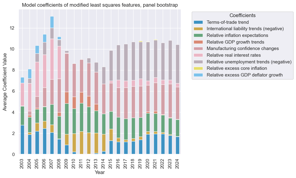
so_mls.coefs_stackedbarplot("MLS_bootstrap", title="Model coefficients of modified least squares features, panel bootstrap", ftrs_renamed=ftrs_dict)
Comparison #
xcatx = [
    "MLS_analytic",
    "MLS_white",
    "MLS_bootstrap",
    "LS"
]
cidx = cids_dmfx

msp.view_timelines(
    df = dfx,
    xcats = xcatx,
    cids = cidx,
    title="Signals based on adjusted factor coefficients",
    xcat_labels=["Defacto", "White", "Panel bootstrap", "Unadjusted"]
)
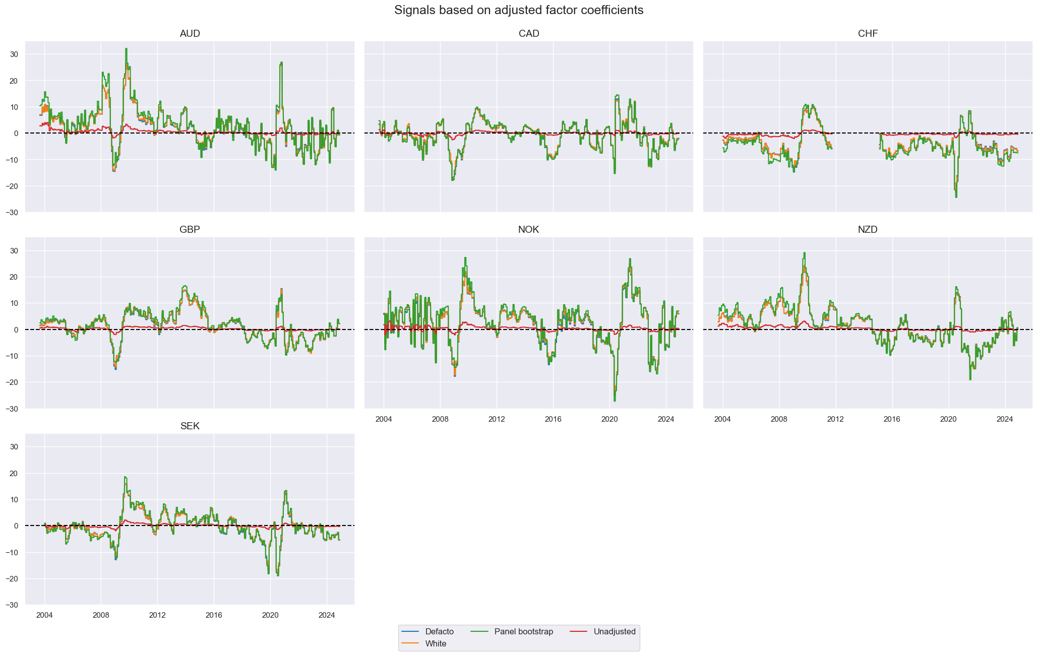
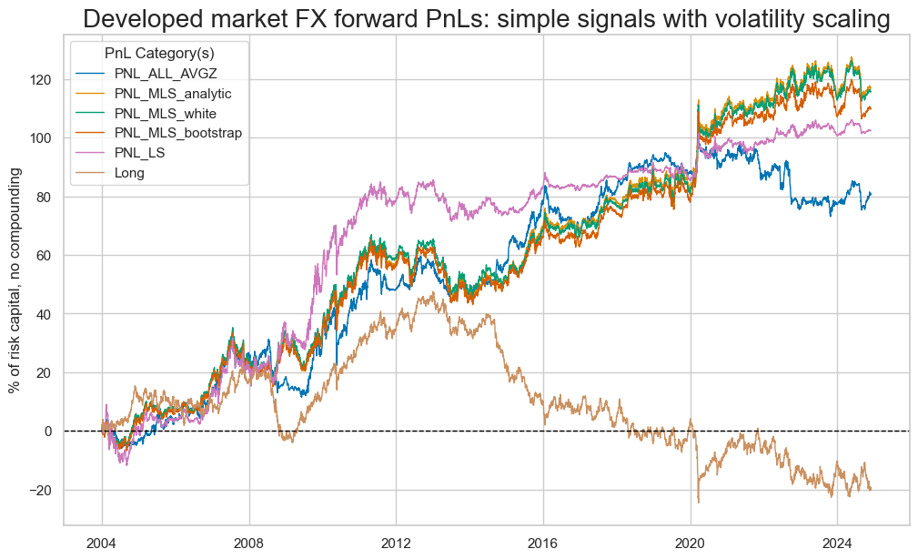
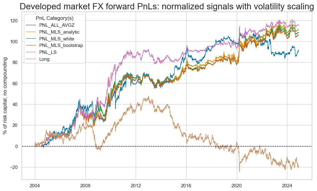
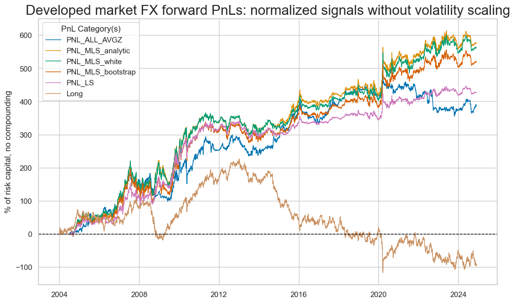
By adjusting the coefficients, the value generated in the early history is mitigated - as hoped - resulting in more consistent PnL generation over the 20 years. A consequence of adjusting by statistical precision is that one is able to take greater advantage of more recent periods where there is a clear long/short signal, instead of the signal petering out over time.
sigx = [
    "ALL_AVGZ",
    "MLS_analytic",
    "MLS_white",
    "MLS_bootstrap",
    "LS",
]

pnl = msn.NaivePnL(
    df = dfx,
    ret = "FXXR_VT10",
    cids=cids_dmfx,
    sigs = sigx,
    blacklist=fxblack,
    start="2004-01-01",
    bms=["USD_GB10YXR_NSA", "EUR_FXXR_NSA", "USD_EQXR_NSA"],
)

pnl.make_long_pnl(vol_scale=10,label="Long")
for sig in sigx:
    pnl.make_pnl(
        sig = sig,
        sig_op="raw",
        rebal_freq="monthly",
        rebal_slip=1,
        vol_scale=10,
        thresh=5
    )

pnames = ["PNL_" + sig for sig in sigx] + ["Long"]
pnl.plot_pnls(
    pnl_cats=pnames,
    title="Developed market FX forward PnLs: simple signals with volatility scaling",
)
pnl.evaluate_pnls(pnl_cats=pnames)
| xcat | Long | PNL_ALL_AVGZ | PNL_MLS_analytic | PNL_MLS_white | PNL_MLS_bootstrap | PNL_LS |
|---|---|---|---|---|---|---|
| Return % | -0.92455 | 3.864559 | 5.595817 | 5.535685 | 5.25837 | 4.895306 |
| St. Dev. % | 10.0 | 10.0 | 10.0 | 10.0 | 10.0 | 10.0 |
| Sharpe Ratio | -0.092455 | 0.386456 | 0.559582 | 0.553569 | 0.525837 | 0.489531 |
| Sortino Ratio | -0.126782 | 0.53985 | 0.787278 | 0.778566 | 0.737231 | 0.681116 |
| Max 21-Day Draw % | -23.065732 | -19.618452 | -13.822903 | -13.888335 | -13.41565 | -16.766195 |
| Max 6-Month Draw % | -22.801123 | -14.746112 | -18.166749 | -18.506355 | -18.51456 | -17.025071 |
| Peak to Trough Draw % | -72.053121 | -30.033006 | -21.351394 | -21.114831 | -22.354549 | -20.880637 |
| Top 5% Monthly PnL Share | -3.836347 | 0.97085 | 0.664541 | 0.665043 | 0.696498 | 0.717804 |
| USD_GB10YXR_NSA correl | -0.013323 | -0.091145 | -0.077103 | -0.081348 | -0.083263 | -0.06613 |
| EUR_FXXR_NSA correl | 0.409057 | 0.136722 | 0.060172 | 0.066599 | 0.074526 | 0.149307 |
| USD_EQXR_NSA correl | 0.248706 | 0.124388 | -0.003433 | 0.00293 | 0.012423 | 0.053996 |
| Traded Months | 251 | 251 | 251 | 251 | 251 | 251 |
sigx = [
    "ALL_AVGZ",
    "MLS_analytic",
    "MLS_white",
    "MLS_bootstrap",
    "LS",
]

pnl = msn.NaivePnL(
    df = dfx,
    ret = "FXXR_VT10",
    cids=cids_dmfx,
    sigs = sigx,
    blacklist=fxblack,
    start="2004-01-01",
    bms=["USD_GB10YXR_NSA", "EUR_FXXR_NSA", "USD_EQXR_NSA"],
)

pnl.make_long_pnl(vol_scale=10,label="Long")
for sig in sigx:
    pnl.make_pnl(
        sig = sig,
        sig_op="zn_score_pan",
        min_obs=22 * 6,  # minimum required data for normalization
        iis=False,  # allow no in-sample bias
        rebal_freq="monthly",
        rebal_slip=1,
        vol_scale=10,
        thresh=4
    )

pnames = ["PNL_" + sig for sig in sigx] + ["Long"]
pnl.plot_pnls(
    pnl_cats=pnames,
    title="Developed market FX forward PnLs: normalized signals with volatility scaling",
)
pnl.evaluate_pnls(pnl_cats=pnames)
| xcat | Long | PNL_ALL_AVGZ | PNL_MLS_analytic | PNL_MLS_white | PNL_MLS_bootstrap | PNL_LS |
|---|---|---|---|---|---|---|
| Return % | -0.92455 | 4.46374 | 5.430595 | 5.300886 | 5.183684 | 5.666545 |
| St. Dev. % | 10.0 | 10.0 | 10.0 | 10.0 | 10.0 | 10.0 |
| Sharpe Ratio | -0.092455 | 0.446374 | 0.543059 | 0.530089 | 0.518368 | 0.566654 |
| Sortino Ratio | -0.126782 | 0.63411 | 0.778092 | 0.75818 | 0.740538 | 0.810898 |
| Max 21-Day Draw % | -23.065732 | -17.656563 | -13.688723 | -14.043633 | -13.782562 | -15.397057 |
| Max 6-Month Draw % | -22.801123 | -14.699633 | -16.764413 | -16.98785 | -16.227148 | -15.456484 |
| Peak to Trough Draw % | -72.053121 | -30.089127 | -20.009813 | -20.206334 | -21.311656 | -18.527638 |
| Top 5% Monthly PnL Share | -3.836347 | 0.848994 | 0.66864 | 0.672063 | 0.670756 | 0.646396 |
| USD_GB10YXR_NSA correl | -0.013323 | -0.095306 | -0.075816 | -0.083268 | -0.092189 | -0.088641 |
| EUR_FXXR_NSA correl | 0.409057 | 0.128249 | 0.057387 | 0.066144 | 0.088598 | 0.105078 |
| USD_EQXR_NSA correl | 0.248706 | 0.122349 | -0.013755 | -0.003922 | 0.018741 | 0.032487 |
| Traded Months | 251 | 251 | 251 | 251 | 251 | 251 |
sigx = [
    "ALL_AVGZ",
    "MLS_analytic",
    "MLS_white",
    "MLS_bootstrap",
    "LS",
]

pnl = msn.NaivePnL(
    df = dfx,
    ret = "FXXR_VT10",
    cids=cids_dmfx,
    sigs = sigx,
    blacklist=fxblack,
    start="2004-01-01",
    bms=["USD_GB10YXR_NSA", "EUR_FXXR_NSA", "USD_EQXR_NSA"],
)

pnl.make_long_pnl(label="Long")
for sig in sigx:
    pnl.make_pnl(
        sig = sig,
        sig_op="zn_score_pan",
        min_obs=22 * 6,  # minimum required data for normalization
        iis=False,  # allow no in-sample bias
        rebal_freq="monthly",
        rebal_slip=1,
        thresh=4
    )

pnames = ["PNL_" + sig for sig in sigx] + ["Long"]
pnl.plot_pnls(
    pnl_cats=pnames,
    title="Developed market FX forward PnLs: normalized signals without volatility scaling",
)
pnl.evaluate_pnls(pnl_cats=pnames)
| xcat | Long | PNL_ALL_AVGZ | PNL_MLS_analytic | PNL_MLS_white | PNL_MLS_bootstrap | PNL_LS |
|---|---|---|---|---|---|---|
| Return % | -4.403992 | 19.007053 | 28.184664 | 27.519177 | 25.42674 | 20.916911 |
| St. Dev. % | 47.633919 | 42.581008 | 51.899774 | 51.914301 | 49.051481 | 36.912991 |
| Sharpe Ratio | -0.092455 | 0.446374 | 0.543059 | 0.530089 | 0.518368 | 0.566654 |
| Sortino Ratio | -0.126782 | 0.63411 | 0.778092 | 0.75818 | 0.740538 | 0.810898 |
| Max 21-Day Draw % | -109.871121 | -75.183425 | -71.044161 | -72.906542 | -67.605505 | -56.835144 |
| Max 6-Month Draw % | -108.610685 | -62.592519 | -87.006926 | -88.191237 | -79.596562 | -57.054505 |
| Peak to Trough Draw % | -343.21725 | -128.122537 | -103.850474 | -104.899769 | -104.536827 | -68.391055 |
| Top 5% Monthly PnL Share | -3.836347 | 0.848994 | 0.66864 | 0.672063 | 0.670756 | 0.646396 |
| USD_GB10YXR_NSA correl | -0.013323 | -0.095306 | -0.075816 | -0.083268 | -0.092189 | -0.088641 |
| EUR_FXXR_NSA correl | 0.409057 | 0.128249 | 0.057387 | 0.066144 | 0.088598 | 0.105078 |
| USD_EQXR_NSA correl | 0.248706 | 0.122349 | -0.013755 | -0.003922 | 0.018741 | 0.032487 |
| Traded Months | 251 | 251 | 251 | 251 | 251 | 251 |
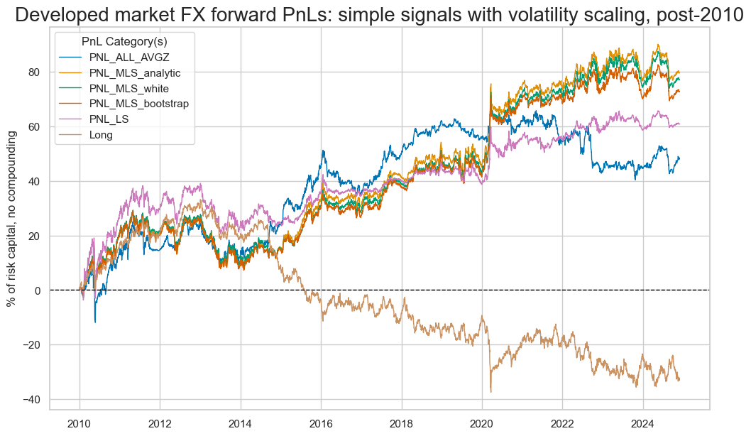
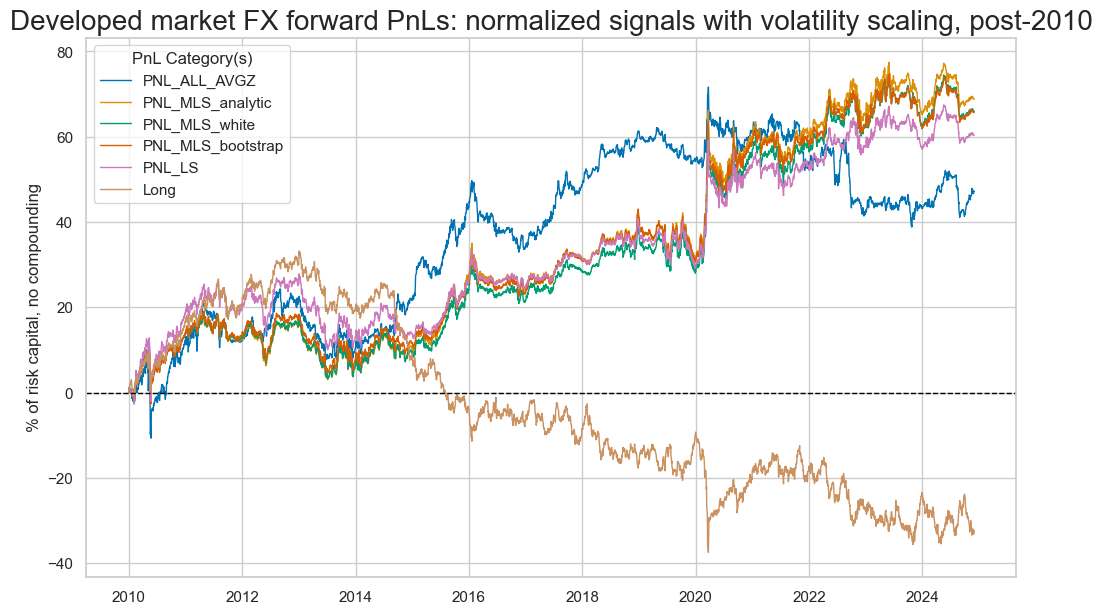
The coefficients for the unadjusted OLS-based signal noticeably diminished post-2010. A comparison between the adjusted and unadjusted OLS signals in this period revealed substantial outperformance of the adjusted signal in this period.
sigx = [
    "ALL_AVGZ",
    "MLS_analytic",
    "MLS_white",
    "MLS_bootstrap",
    "LS",
]

pnl = msn.NaivePnL(
    df = dfx,
    ret = "FXXR_VT10",
    cids=cids_dmfx,
    sigs = sigx,
    blacklist=fxblack,
    start="2010-01-01",
    bms=["USD_GB10YXR_NSA", "EUR_FXXR_NSA", "USD_EQXR_NSA"],
)

pnl.make_long_pnl(vol_scale=10,label="Long")
for sig in sigx:
    pnl.make_pnl(
        sig = sig,
        sig_op="raw",
        rebal_freq="monthly",
        rebal_slip=1,
        vol_scale=10,
        thresh=5
    )

pnames = ["PNL_" + sig for sig in sigx] + ["Long"]
pnl.plot_pnls(
    pnl_cats=pnames,
    title="Developed market FX forward PnLs: simple signals with volatility scaling, post-2010",
)
pnl.evaluate_pnls(pnl_cats=pnames)
| xcat | Long | PNL_ALL_AVGZ | PNL_MLS_analytic | PNL_MLS_white | PNL_MLS_bootstrap | PNL_LS |
|---|---|---|---|---|---|---|
| Return % | -2.16832 | 3.240884 | 5.345692 | 5.178884 | 4.887603 | 4.084634 |
| St. Dev. % | 10.0 | 10.0 | 10.0 | 10.0 | 10.0 | 10.0 |
| Sharpe Ratio | -0.216832 | 0.324088 | 0.534569 | 0.517888 | 0.48876 | 0.408463 |
| Sortino Ratio | -0.294356 | 0.448844 | 0.759138 | 0.734478 | 0.69064 | 0.56178 |
| Max 21-Day Draw % | -22.621368 | -20.229224 | -13.596687 | -13.630355 | -13.158314 | -21.787402 |
| Max 6-Month Draw % | -19.717585 | -14.10706 | -17.869444 | -18.162593 | -18.159418 | -17.801421 |
| Peak to Trough Draw % | -70.665007 | -30.968011 | -21.001971 | -20.722616 | -21.925749 | -22.100723 |
| Top 5% Monthly PnL Share | -1.622954 | 1.217846 | 0.710515 | 0.724512 | 0.769286 | 0.93927 |
| USD_GB10YXR_NSA correl | 0.015664 | -0.075037 | -0.114884 | -0.119936 | -0.120414 | -0.113668 |
| EUR_FXXR_NSA correl | 0.326556 | 0.123358 | 0.011575 | 0.021055 | 0.031531 | 0.096827 |
| USD_EQXR_NSA correl | 0.296793 | 0.127985 | -0.007362 | 0.001926 | 0.011431 | 0.060877 |
| Traded Months | 179 | 179 | 179 | 179 | 179 | 179 |
sigx = [
    "ALL_AVGZ",
    "MLS_analytic",
    "MLS_white",
    "MLS_bootstrap",
    "LS",
]

pnl = msn.NaivePnL(
    df = dfx,
    ret = "FXXR_VT10",
    cids=cids_dmfx,
    sigs = sigx,
    blacklist=fxblack,
    start="2010-01-01",
    bms=["USD_GB10YXR_NSA", "EUR_FXXR_NSA", "USD_EQXR_NSA"],
)

pnl.make_long_pnl(vol_scale=10,label="Long")
for sig in sigx:
    pnl.make_pnl(
        sig = sig,
        sig_op="zn_score_pan",
        rebal_freq="monthly",
        rebal_slip=1,
        vol_scale=10,
        thresh=4
    )

pnames = ["PNL_" + sig for sig in sigx] + ["Long"]
pnl.plot_pnls(
    pnl_cats=pnames,
    title="Developed market FX forward PnLs: normalized signals with volatility scaling, post-2010",
)
pnl.evaluate_pnls(pnl_cats=pnames)
| xcat | Long | PNL_ALL_AVGZ | PNL_MLS_analytic | PNL_MLS_white | PNL_MLS_bootstrap | PNL_LS |
|---|---|---|---|---|---|---|
| Return % | -2.16832 | 3.161544 | 4.621014 | 4.425778 | 4.41232 | 4.050096 |
| St. Dev. % | 10.0 | 10.0 | 10.0 | 10.0 | 10.0 | 10.0 |
| Sharpe Ratio | -0.216832 | 0.316154 | 0.462101 | 0.442578 | 0.441232 | 0.40501 |
| Sortino Ratio | -0.294356 | 0.440384 | 0.661945 | 0.632144 | 0.627057 | 0.569836 |
| Max 21-Day Draw % | -22.621368 | -17.846605 | -12.010833 | -12.137633 | -12.445161 | -14.773203 |
| Max 6-Month Draw % | -19.717585 | -14.614635 | -13.385832 | -13.540575 | -13.368312 | -17.151638 |
| Peak to Trough Draw % | -70.665007 | -32.82331 | -17.37586 | -17.347939 | -16.695269 | -17.784512 |
| Top 5% Monthly PnL Share | -1.622954 | 1.257381 | 0.824436 | 0.83956 | 0.864626 | 0.888809 |
| USD_GB10YXR_NSA correl | 0.015664 | -0.072937 | -0.101714 | -0.108693 | -0.108015 | -0.111363 |
| EUR_FXXR_NSA correl | 0.326556 | 0.113491 | 0.00091 | 0.004608 | 0.020234 | 0.052105 |
| USD_EQXR_NSA correl | 0.296793 | 0.120792 | -0.04605 | -0.037737 | -0.020693 | 0.002524 |
| Traded Months | 179 | 179 | 179 | 179 | 179 | 179 |
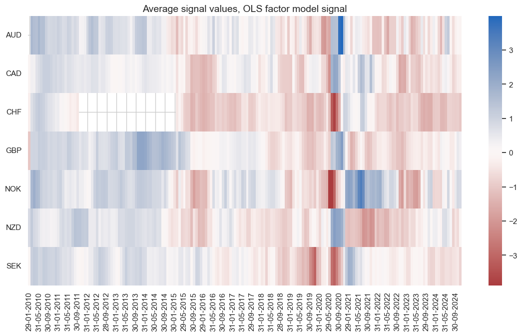
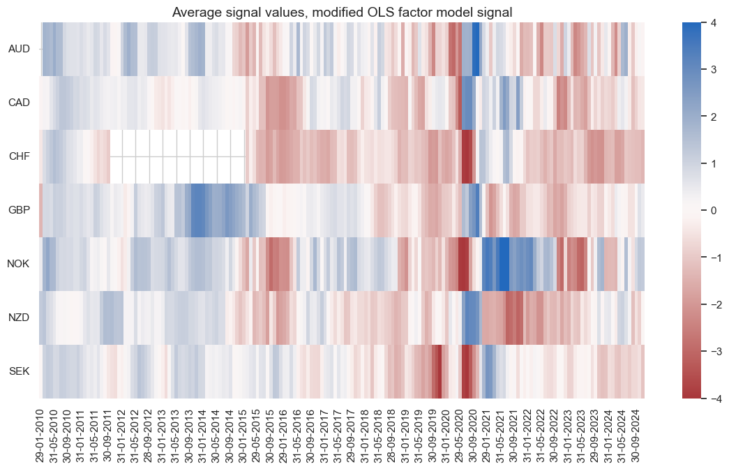
We see below that the signals from the unadjusted models vanished over time, whilst the adjusted versions are able to produce strong signals in the more recent past.
pnl.signal_heatmap(
    pnl_name="PNL_LS",
    title="Average signal values, OLS factor model signal"
)
pnl.signal_heatmap(
    pnl_name="PNL_MLS_analytic",
    title="Average signal values, modified OLS factor model signal"
)
