Macroeconomic cycles and asset class returns

This notebook offers the necessary code to replicate the research findings discussed in Macrosynergy’s post “Macroeconomic cycles and asset class returns” . Its primary objective is to inspire readers to explore and conduct additional investigations while also providing a foundation for testing their own unique ideas.

Get packages and JPMaQS data

This notebook primarily relies on the standard packages available in the Python data science stack. However, there is an additional package macrosynergy that is required for two purposes:

• Downloading JPMaQS data: The macrosynergy package facilitates the retrieval of JPMaQS data, which is used in the notebook.

• For the analysis of quantamental data and value propositions: The macrosynergy package provides functionality for performing quick analyses of quantamental data and exploring value propositions.

For detailed information and a comprehensive understanding of the macrosynergy package and its functionalities, please refer to the “Introduction to Macrosynergy package” on the Macrosynergy Academy or visit the following link on Kaggle .

import numpy as np
import pandas as pd
import matplotlib.pyplot as plt
import seaborn as sns


import macrosynergy.management as msm
import macrosynergy.panel as msp
import macrosynergy.signal as mss
import macrosynergy.pnl as msn
from macrosynergy.download import JPMaQSDownload

from datetime import timedelta, date, datetime
from itertools import combinations
import warnings
import os

warnings.simplefilter("ignore")

The JPMaQS indicators we consider are downloaded using the J.P. Morgan Dataquery API interface within the macrosynergy package. This is done by specifying ticker strings, formed by appending an indicator category code to a currency area code <cross_section>. These constitute the main part of a full quantamental indicator ticker, taking the form DB(JPMAQS,<cross_section>_<category>,<info>) , where denotes the time series of information for the given cross-section and category. The following types of information are available:

value giving the latest available values for the indicator eop_lag referring to days elapsed since the end of the observation period mop_lag referring to the number of days elapsed since the mean observation period grade denoting a grade of the observation, giving a metric of real time information quality.

After instantiating the JPMaQSDownload class within the macrosynergy.download module, one can use the download(tickers,start_date,metrics) method to easily download the necessary data, where tickers is an array of ticker strings, start_date is the first collection date to be considered and metrics is an array comprising the times series information to be downloaded. For more information see here .

To ensure reproducibility, only samples between January 2000 (inclusive) and May 2023 (exclusive) are considered.

# General cross-sections lists

cids_g3 = ["EUR", "JPY", "USD"]  # DM large currency areas
cids_dmsc = ["AUD", "CAD", "CHF", "GBP", "NOK", "NZD", "SEK"]  # DM small currency areas
cids_latm = ["BRL", "COP", "CLP", "MXN", "PEN"]  # Latam
cids_emea = ["CZK", "HUF", "ILS", "PLN", "RON", "RUB", "TRY", "ZAR"]  # EMEA
cids_emas = ["IDR", "INR", "KRW", "MYR", "PHP", "SGD", "THB", "TWD"]  # EM Asia ex China

cids_dm = cids_g3 + cids_dmsc
cids_em = cids_latm + cids_emea + cids_emas
cids = cids_dm + cids_em

cids_nomp = ["COP", "IDR", "INR"]  # countries that have no employment growth data
cids_mp = list(set(cids) - set(cids_nomp))

# Equity cross-sections lists

cids_dmeq = ["EUR", "JPY", "USD"] + ["AUD", "CAD", "CHF", "GBP", "SEK"]
cids_emeq = ["BRL", "INR", "KRW", "MXN", "MYR", "SGD", "THB", "TRY", "TWD", "ZAR"]
cids_eq = cids_dmeq + cids_emeq

# FX cross-sections lists

cids_nofx = ["EUR", "USD", "SGD"]
cids_fx = list(set(cids) - set(cids_nofx))

cids_dmfx = set(cids_dm).intersection(cids_fx)
cids_emfx = set(cids_em).intersection(cids_fx)

cids_eur = ["CHF", "CZK", "HUF", "NOK", "PLN", "RON", "SEK"]  # trading against EUR
cids_eud = ["GBP", "RUB", "TRY"]  # trading against EUR and USD
cids_usd = list(set(cids_fx) - set(cids_eur + cids_eud))  # trading against USD

# IRS cross-section lists

cids_dmsc_du = ["AUD", "CAD", "CHF", "GBP", "NOK", "NZD", "SEK"]
cids_latm_du = ["CLP", "COP", "MXN"]  # Latam
cids_emea_du = [
    "CZK",
    "HUF",
    "ILS",
    "PLN",
    "RON",
    "RUB",
    "TRY",
    "ZAR",
]  # EMEA
cids_emas_du = ["CNY", "HKD", "IDR", "INR", "KRW", "MYR", "SGD", "THB", "TWD"]

cids_dmdu = cids_g3 + cids_dmsc_du
cids_emdu = cids_latm_du + cids_emea_du + cids_emas_du
cids_du = cids_dmdu + cids_emdu

JPMaQS indicators are conveniently grouped into 6 main categories: Economic Trends, Macroeconomic balance sheets, Financial conditions, Shocks and risk measures, Stylyzed trading factors, and Generic returns. Each indicator has a separate page with notes, description, availability, statistical measures, and timelines for main currencies. The description of each JPMaQS category is available either under Macro Quantamental Academy , JPMorgan Markets (password protected). In particular, the indicators used in this notebook could be found under Labor market dynamics , Demographic trends , Consumer price inflation trends , Intuitive growth estimates , Long-term GDP growth , Private credit expansion , Equity index future returns , FX forward returns , and Duration returns .

# Category tickers

main = [
    "EMPL_NSA_P1M1ML12_3MMA",
    "EMPL_NSA_P1Q1QL4",
    "WFORCE_NSA_P1Y1YL1_5YMM",
    "WFORCE_NSA_P1Q1QL4_20QMM",
    "UNEMPLRATE_NSA_3MMA_D1M1ML12",
    "UNEMPLRATE_NSA_D1Q1QL4",
    "UNEMPLRATE_SA_D1Q1QL4",  # potentially NZD only
    "UNEMPLRATE_SA_D3M3ML3",
    "UNEMPLRATE_SA_D1Q1QL1",
    "UNEMPLRATE_SA_3MMA",
    "UNEMPLRATE_SA_3MMAv10YMM",
    "CPIH_SA_P1M1ML12",
    "CPIH_SJA_P6M6ML6AR",
    "CPIC_SA_P1M1ML12",
    "CPIC_SJA_P6M6ML6AR",
    "INFTEFF_NSA",
    "INTRGDPv5Y_NSA_P1M1ML12_3MMA",
    "RGDP_SA_P1Q1QL4_20QMM",
    "PCREDITBN_SJA_P1M1ML12",
]
xtra = ["GB10YXR_NSA"]

rets = [
    "EQXR_NSA",
    "EQXR_VT10",
    "FXTARGETED_NSA",
    "FXUNTRADABLE_NSA",
    "FXXR_NSA",
    "FXXR_VT10",
    "FXXRHvGDRB_NSA",
    "DU02YXR_NSA",
    "DU02YXR_VT10",
    "DU05YXR_VT10",
]

xcats = main + rets + xtra

# Download series from J.P. Morgan DataQuery by tickers

start_date = "2000-01-01"
end_date = "2023-05-01"

tickers = [cid + "_" + xcat for cid in cids for xcat in xcats]
print(f"Maximum number of tickers is {len(tickers)}")

# Retrieve credentials

client_id: str = os.getenv("DQ_CLIENT_ID")
client_secret: str = os.getenv("DQ_CLIENT_SECRET")

with JPMaQSDownload(client_id=client_id, client_secret=client_secret) as dq:
    df = dq.download(
        tickers=tickers,
        start_date=start_date,
        suppress_warning=True,
        metrics=["value"],
        report_time_taken=True,
        show_progress=True,
    )

Maximum number of tickers is 930
Downloading data from JPMaQS.
Timestamp UTC:  2024-11-19 09:42:46
Connection successful!

Requesting data: 100%|██████████| 47/47 [00:09<00:00,  4.84it/s]
Downloading data: 100%|██████████| 47/47 [00:11<00:00,  4.21it/s]

Time taken to download data: 	22.68 seconds.
Some expressions are missing from the downloaded data. Check logger output for complete list.
229 out of 930 expressions are missing. To download the catalogue of all available expressions and filter the unavailable expressions, set `get_catalogue=True` in the call to `JPMaQSDownload.download()`.
Some dates are missing from the downloaded data. 
3 out of 6494 dates are missing.

display(df["xcat"].unique())
display(df["cid"].unique())
df["ticker"] = df["cid"] + "_" + df["xcat"]
df.head(3)

array(['FXTARGETED_NSA', 'FXXRHvGDRB_NSA', 'DU02YXR_NSA', 'DU02YXR_VT10',
       'CPIH_SJA_P6M6ML6AR', 'CPIC_SJA_P6M6ML6AR',
       'WFORCE_NSA_P1Y1YL1_5YMM', 'INTRGDPv5Y_NSA_P1M1ML12_3MMA',
       'EQXR_VT10', 'DU05YXR_VT10', 'FXUNTRADABLE_NSA', 'FXXR_VT10',
       'INFTEFF_NSA', 'FXXR_NSA', 'PCREDITBN_SJA_P1M1ML12',
       'RGDP_SA_P1Q1QL4_20QMM', 'EQXR_NSA', 'CPIH_SA_P1M1ML12',
       'CPIC_SA_P1M1ML12', 'UNEMPLRATE_SA_3MMAv10YMM',
       'UNEMPLRATE_SA_D1Q1QL1', 'EMPL_NSA_P1Q1QL4', 'UNEMPLRATE_SA_3MMA',
       'UNEMPLRATE_NSA_D1Q1QL4', 'EMPL_NSA_P1M1ML12_3MMA',
       'UNEMPLRATE_NSA_3MMA_D1M1ML12', 'UNEMPLRATE_SA_D3M3ML3',
       'GB10YXR_NSA', 'WFORCE_NSA_P1Q1QL4_20QMM'], dtype=object)

array(['INR', 'PHP', 'HUF', 'KRW', 'THB', 'NZD', 'SGD', 'CHF', 'GBP',
       'MXN', 'ZAR', 'TRY', 'COP', 'RON', 'SEK', 'ILS', 'CLP', 'EUR',
       'AUD', 'JPY', 'USD', 'CAD', 'CZK', 'NOK', 'PLN', 'MYR', 'PEN',
       'IDR', 'TWD', 'RUB', 'BRL'], dtype=object)

	real_date	cid	xcat	value	ticker
0	2000-01-03	INR	FXTARGETED_NSA	1.0	INR_FXTARGETED_NSA
1	2000-01-04	INR	FXTARGETED_NSA	1.0	INR_FXTARGETED_NSA
2	2000-01-05	INR	FXTARGETED_NSA	1.0	INR_FXTARGETED_NSA

scols = ["cid", "xcat", "real_date", "value"]  # required columns
dfx = df[scols].copy()
dfx.info()

<class 'pandas.core.frame.DataFrame'>
RangeIndex: 4302461 entries, 0 to 4302460
Data columns (total 4 columns):
 #   Column     Dtype         
---  ------     -----         
 0   cid        object        
 1   xcat       object        
 2   real_date  datetime64[ns]
 3   value      float64       
dtypes: datetime64[ns](1), float64(1), object(2)
memory usage: 131.3+ MB

Blacklist dictionaries

Identifying and isolating periods of official exchange rate targets, illiquidity, or convertibility-related distortions in FX markets is the first step in creating an FX trading strategy. These periods can significantly impact the behavior and dynamics of currency markets, and failing to account for them can lead to inaccurate or misleading findings.

dfb = df[df["xcat"].isin(["FXTARGETED_NSA", "FXUNTRADABLE_NSA"])].loc[
    :, ["cid", "xcat", "real_date", "value"]
]
dfba = (
    dfb.groupby(["cid", "real_date"])
    .aggregate(value=pd.NamedAgg(column="value", aggfunc="max"))
    .reset_index()
)
dfba["xcat"] = "FXBLACK"
fxblack = msp.make_blacklist(dfba, "FXBLACK")
fxblack

{'BRL': (Timestamp('2012-12-03 00:00:00'), Timestamp('2013-09-30 00:00:00')),
 'CHF': (Timestamp('2011-10-03 00:00:00'), Timestamp('2015-01-30 00:00:00')),
 'CZK': (Timestamp('2014-01-01 00:00:00'), Timestamp('2017-07-31 00:00:00')),
 'ILS': (Timestamp('2000-01-03 00:00:00'), Timestamp('2005-12-30 00:00:00')),
 'INR': (Timestamp('2000-01-03 00:00:00'), Timestamp('2004-12-31 00:00:00')),
 'MYR_1': (Timestamp('2000-01-03 00:00:00'), Timestamp('2007-11-30 00:00:00')),
 'MYR_2': (Timestamp('2018-07-02 00:00:00'), Timestamp('2024-11-18 00:00:00')),
 'PEN': (Timestamp('2021-07-01 00:00:00'), Timestamp('2021-07-30 00:00:00')),
 'RON': (Timestamp('2000-01-03 00:00:00'), Timestamp('2005-11-30 00:00:00')),
 'RUB_1': (Timestamp('2000-01-03 00:00:00'), Timestamp('2005-11-30 00:00:00')),
 'RUB_2': (Timestamp('2022-02-01 00:00:00'), Timestamp('2024-11-18 00:00:00')),
 'SGD': (Timestamp('2000-01-03 00:00:00'), Timestamp('2024-11-18 00:00:00')),
 'THB': (Timestamp('2007-01-01 00:00:00'), Timestamp('2008-11-28 00:00:00')),
 'TRY_1': (Timestamp('2000-01-03 00:00:00'), Timestamp('2003-09-30 00:00:00')),
 'TRY_2': (Timestamp('2020-01-01 00:00:00'), Timestamp('2024-07-31 00:00:00'))}

dublack = {
    "TRY": fxblack["TRY_2"]
}  # create a customized blacklist for TRY to be used later in the code

Availability

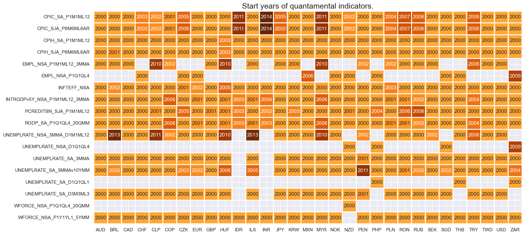
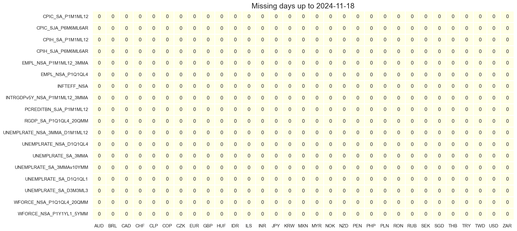
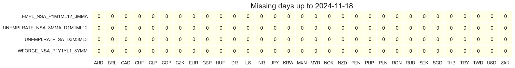
It is important to assess data availability before conducting any analysis. It allows to identify any potential gaps or limitations in the dataset, which can impact the validity and reliability of analysis and ensure that a sufficient number of observations for each selected category and cross-section is available as well as determining the appropriate time periods for analysis.

msm.check_availability(df, xcats=main, cids=cids)

Transformations and checks

Features

Name replacements

dict_repl = {
    "EMPL_NSA_P1Q1QL4": "EMPL_NSA_P1M1ML12_3MMA",
    "WFORCE_NSA_P1Q1QL4_20QMM": "WFORCE_NSA_P1Y1YL1_5YMM",
    "UNEMPLRATE_NSA_D1Q1QL4": "UNEMPLRATE_NSA_3MMA_D1M1ML12",
    "UNEMPLRATE_SA_D1Q1QL1": "UNEMPLRATE_SA_D3M3ML3",
}

for key, value in dict_repl.items():
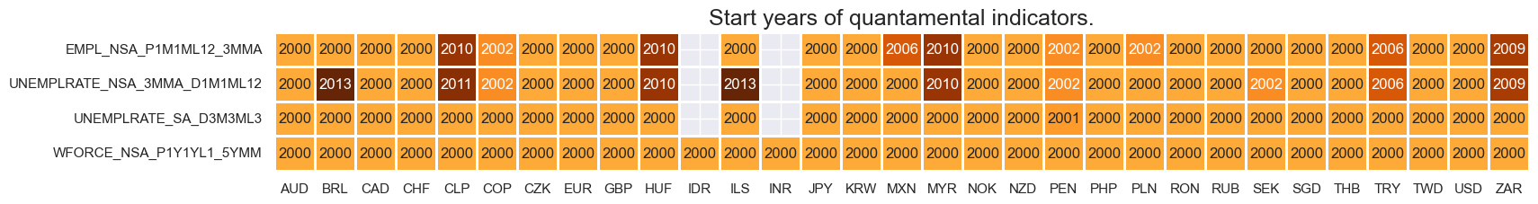
    dfx["xcat"] = dfx["xcat"].str.replace(key, value)

msm.check_availability(dfx, xcats=list(dict_repl.values()), cids=cids)

Labor market scores

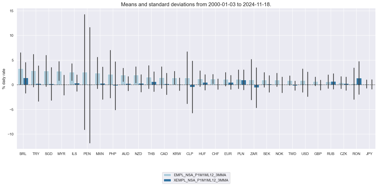
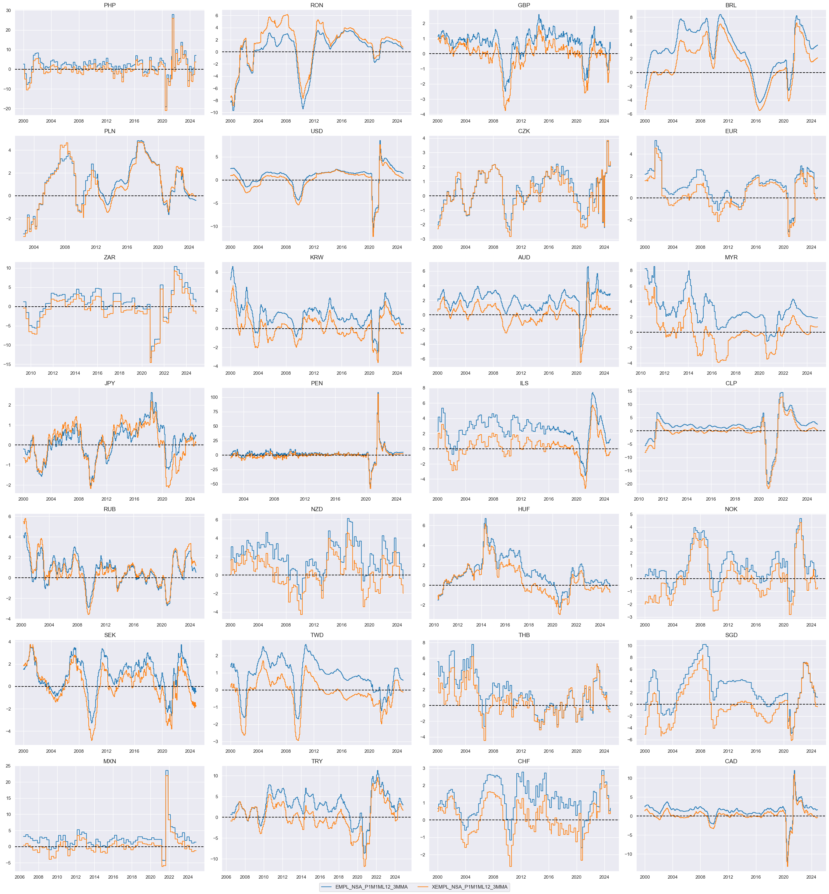
Excess employment growth

To proxy the impact of the business cycle state on employment growth, a common approach is to calculate the difference between employment growth and the long-term median of workforce growth. This difference is often referred to as “excess employment growth.” By calculating excess employment growth, one can estimate the component of employment growth that is attributable to the business cycle state. This measure helps to identify deviations from the long-term trend and provides insights into the cyclical nature of employment dynamics.

calcs = ["XEMPL_NSA_P1M1ML12_3MMA = EMPL_NSA_P1M1ML12_3MMA - WFORCE_NSA_P1Y1YL1_5YMM "]
dfa = msp.panel_calculator(dfx, calcs=calcs, cids=cids, blacklist=None)
dfx = msm.update_df(dfx, dfa)

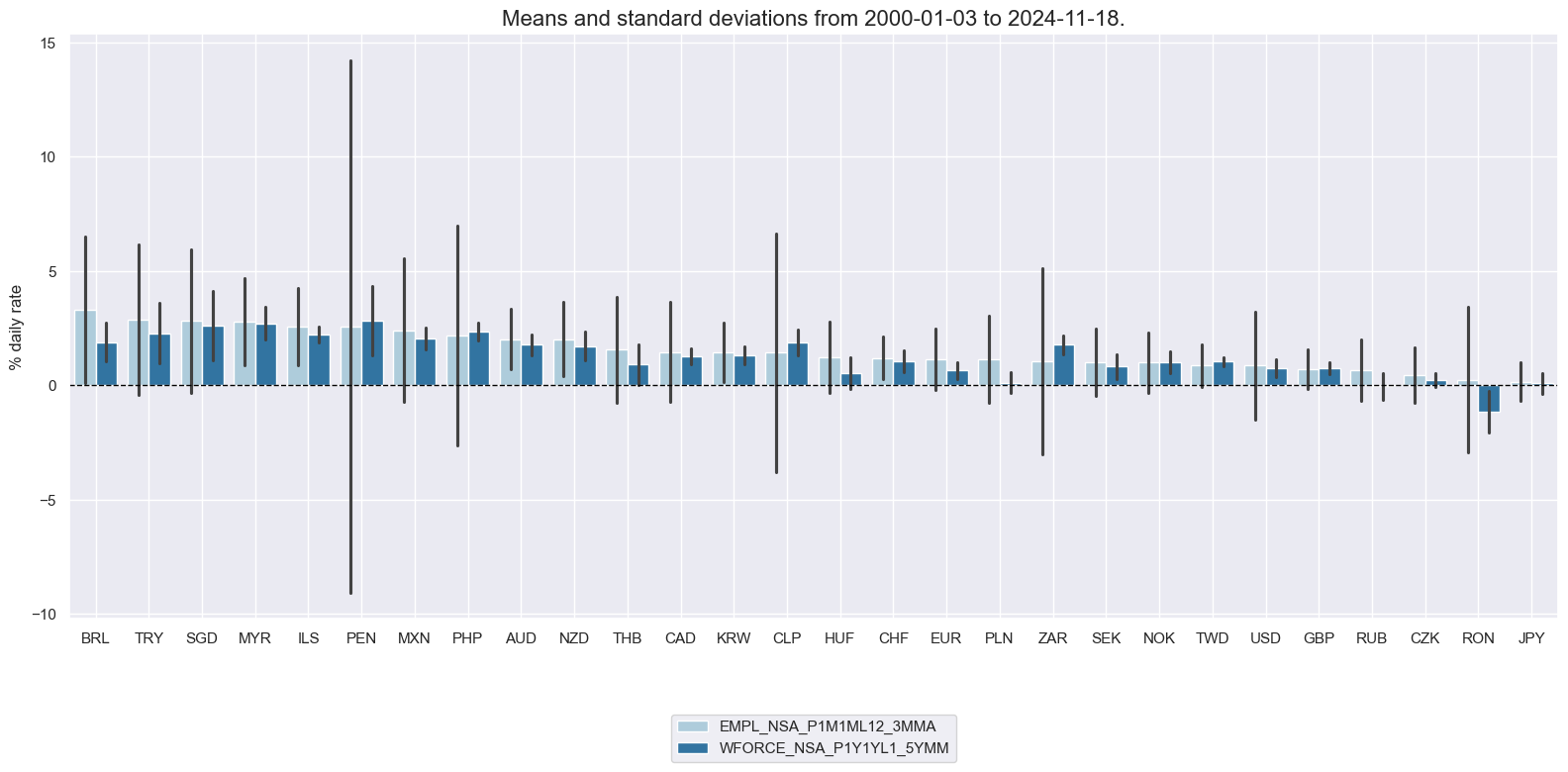
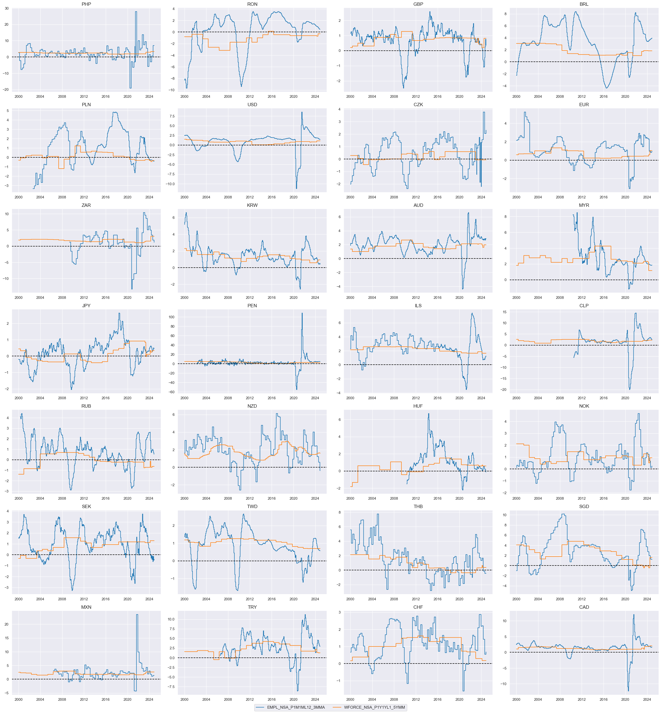
The macrosynergy package provides two useful functions, view_ranges() and view_timelines() , which facilitate the convenient visualization of data for selected indicators and cross-sections. These functions assist in plotting means, standard deviations, and time series of the chosen indicators.

xcatx = ["EMPL_NSA_P1M1ML12_3MMA", "WFORCE_NSA_P1Y1YL1_5YMM"]
cidx = cids_mp

msp.view_ranges(
    dfx,
    cids=cidx,
    xcats=xcatx,
    kind="bar",
    sort_cids_by="mean",
    ylab="% daily rate",
    start="2000-01-01",
)
msp.view_timelines(
    dfx,
    xcats=xcatx,
    cids=cidx,
    ncol=4,
    cumsum=False,
    start="2000-01-01",
    same_y=False,
    size=(12, 12),
    all_xticks=True,

)

xcatx = ["EMPL_NSA_P1M1ML12_3MMA", "XEMPL_NSA_P1M1ML12_3MMA"]
cidx = cids_mp

msp.view_ranges(
    dfx,
    cids=cidx,
    xcats=xcatx,
    kind="bar",
    sort_cids_by="mean",
    ylab="% daily rate",
    start="2000-01-01",
)

msp.view_timelines(
    dfx,
    xcats=xcatx,
    cids=cidx,
    ncol=4,
    cumsum=False,
    start="2000-01-01",
    same_y=False,
    size=(12, 12),
    all_xticks=True,
   )

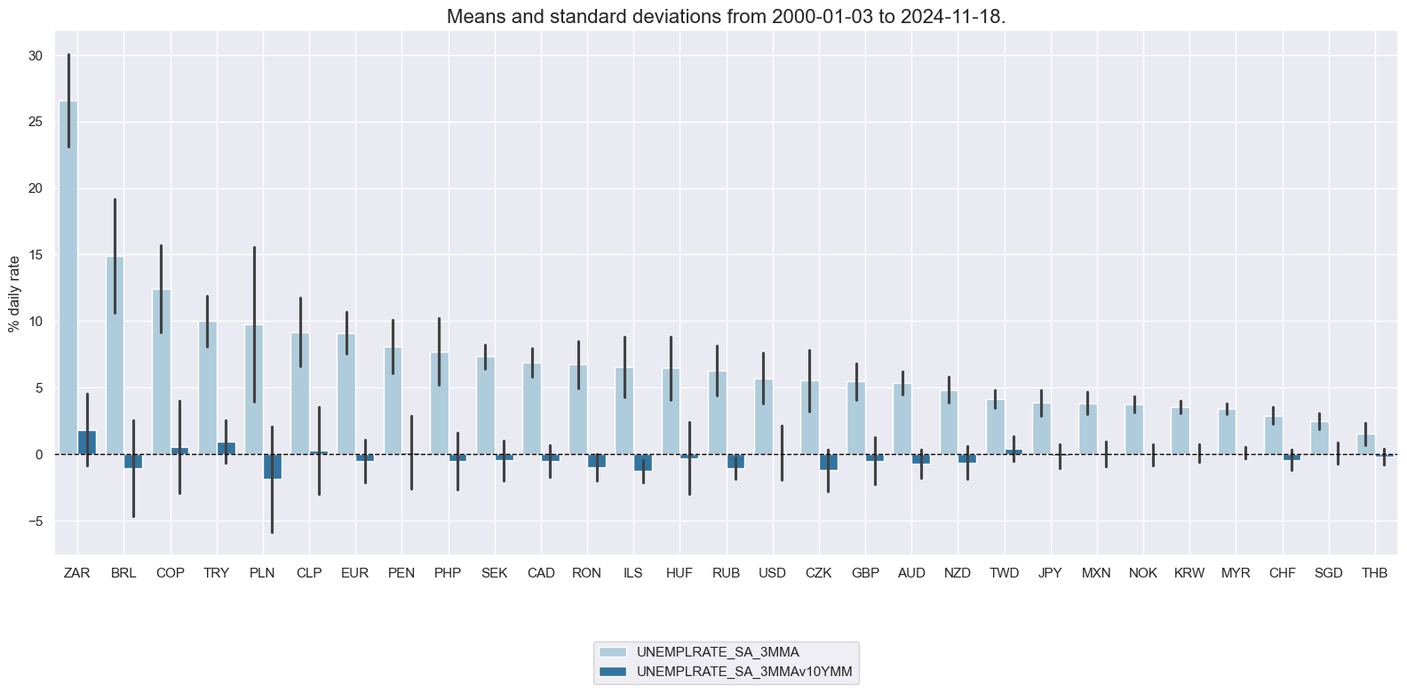
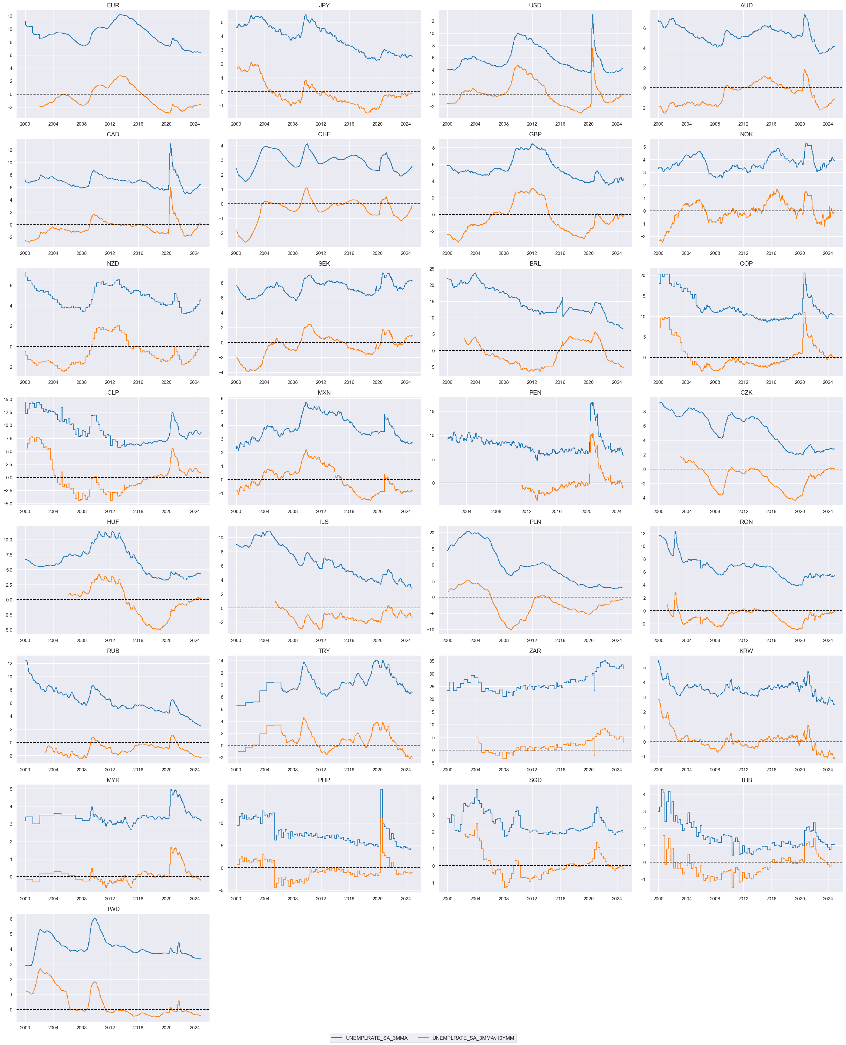
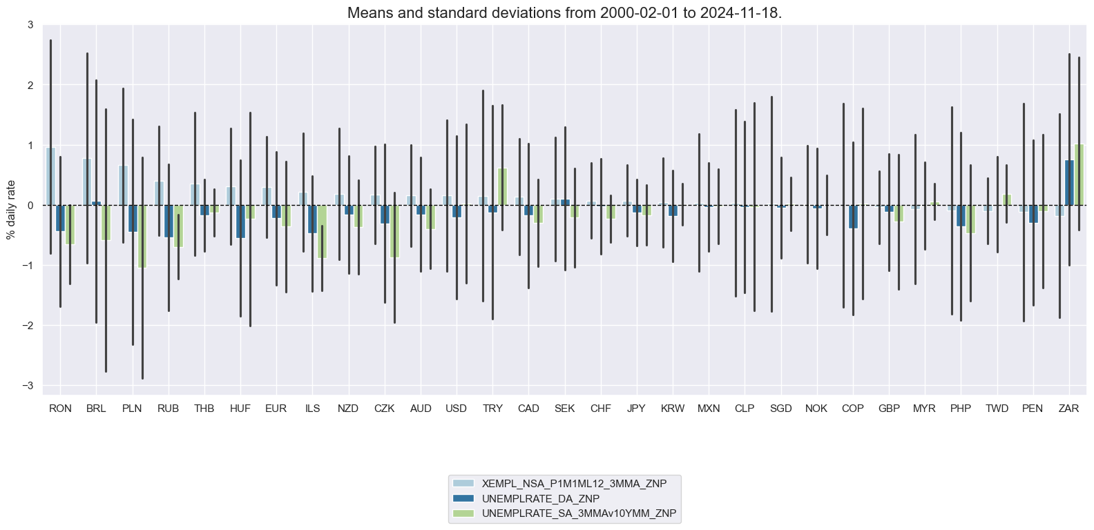
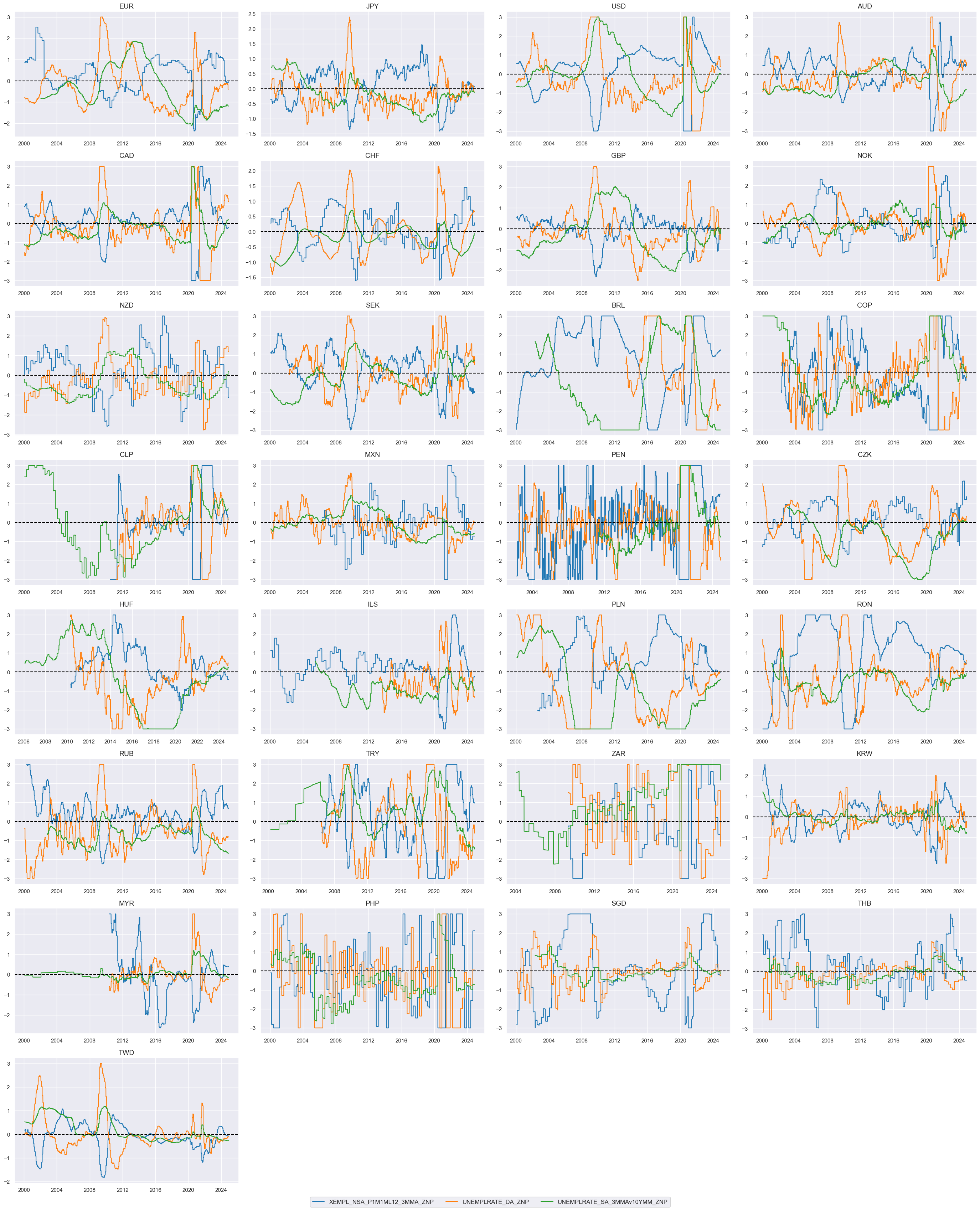
Unemployment rates and gaps

Unemployment rates and unemployment gaps are commonly used measures in labor market analysis. The unemployment rate is a widely used indicator that measures the percentage of the labor force that is unemployed and actively seeking employment. The unemployment gap refers to the difference between the actual unemployment rate and a reference or target unemployment rate. The unemployment gap is used to assess the deviation of the current unemployment rate from the desired or expected level. Here we compare the standard unemployment rate, sa, 3mma with unemployment rate difference, 3-month moving average minus the 10-year moving median. Comparison between the two can give insights into the short-term fluctuations and the long-term trend of the unemployment rate.

xcatx = ["UNEMPLRATE_SA_3MMA", "UNEMPLRATE_SA_3MMAv10YMM"]
cidx = cids

msp.view_ranges(
    dfx,
    cids=cidx,
    xcats=xcatx,
    kind="bar",
    sort_cids_by="mean",
    ylab="% daily rate",
    start="2000-01-01",
)
msp.view_timelines(
    dfx,
    xcats=xcatx,
    cids=cidx,
    ncol=4,
    cumsum=False,
    start="2000-01-01",
    same_y=False,
    size=(12, 12),
    all_xticks=True,
  
)

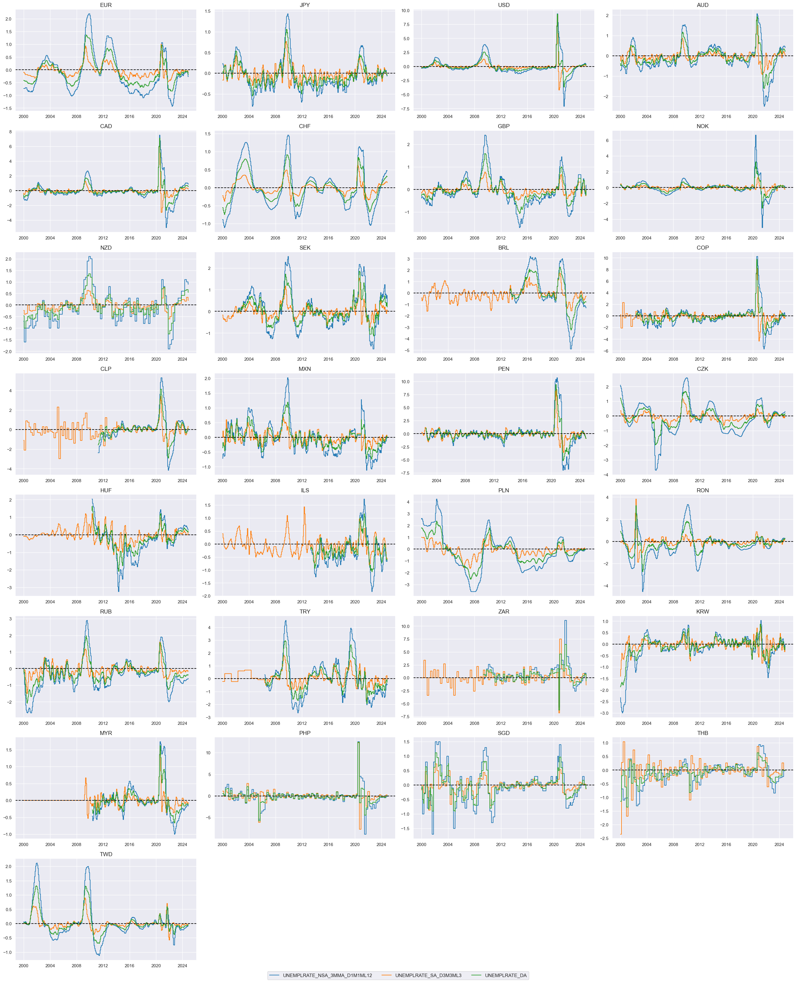
Unemployment changes

We create a simple average of two unemployment growth indicators: unemploent rate change and unemployment growth:

calcs = [
    "UNEMPLRATE_DA = 1/2 * ( UNEMPLRATE_NSA_3MMA_D1M1ML12 + UNEMPLRATE_SA_D3M3ML3 )",
]
dfa = msp.panel_calculator(dfx, calcs=calcs, cids=cids, blacklist=None)
dfx = msm.update_df(dfx, dfa)

xcatx = ["UNEMPLRATE_NSA_3MMA_D1M1ML12", "UNEMPLRATE_SA_D3M3ML3", "UNEMPLRATE_DA"]
cidx = cids

msp.view_timelines(
    dfx,
    xcats=xcatx,
    cids=cidx,
    ncol=4,
    cumsum=False,
    start="2000-01-01",
    same_y=False,
    size=(12, 12),
    all_xticks=True,
 
)

Labor tightening scores

We compute two types of labor market z-scores. One is based on the panel and assumes no structural differences in the features quantitative effects across sections. The other is half based on cross-section alone, which implies persistent structural differences in distributions and their impact on targets. For a description and possible options of function make_zn_scores() please see either Kaggle or under Academy notebooks .

xcat_lab = [
    "XEMPL_NSA_P1M1ML12_3MMA",
    "UNEMPLRATE_DA",
    "UNEMPLRATE_SA_3MMAv10YMM",
]
cidx = msm.common_cids(dfx, xcat_lab)

pws = [0.25, 1]  # cross-sectional and panel-based normalization

for xc in xcat_lab:
    for pw in pws:
        dfa = msp.make_zn_scores(
            dfx,
            xcat=xc,
            cids=cidx,
            sequential=True,
            min_obs=522,  # oos scaling after 2 years of panel data
            est_freq="m",
            neutral="zero",
            pan_weight=pw,
            thresh=3,
            postfix="_ZNP" if pw == 1 else "_ZNM",
        )
        dfx = msm.update_df(dfx, dfa)

The individual category scores are combined into a single labor market tightness score.

xcatx = [
    "XEMPL_NSA_P1M1ML12_3MMA",
    "UNEMPLRATE_DA",
    "UNEMPLRATE_SA_3MMAv10YMM",
]
cidx = msm.common_cids(dfx, xcat_lab)
# cidx.remove("NZD")  # ISSUE: invalid empty series created above
n = len(xcatx)
wx = [1 / n] * n
sx = [1, -1, -1]  # signs for tightening


dix = {"ZNP": [xc + "_ZNP" for xc in xcatx], "ZNM": [xc + "_ZNM" for xc in xcatx]}

dfa = pd.DataFrame(columns=dfx.columns).reindex([])
for key, value in dix.items():
    dfaa = msp.linear_composite(
        dfx,
        xcats=value,
        weights=wx,
        signs=sx,
        cids=cidx,
        complete_xcats=False,  # if some categories are missing the score is based on the remaining
        new_xcat="LABTIGHT_" + key,
    )
    dfa = msm.update_df(dfa, dfaa)
dfx = msm.update_df(dfx, dfa)

xcatx = [xc + "_ZNP" for xc in xcat_lab]
cidx = cids

msp.view_ranges(
    dfx,
    cids=cidx,
    xcats=xcatx,
    kind="bar",
    sort_cids_by="mean",
    ylab="% daily rate",
    start="2000-01-01",
)
msp.view_timelines(
    dfx,
    xcats=xcatx,
    cids=cidx,
    ncol=4,
    cumsum=False,
    start="2000-01-01",
    same_y=False,
    size=(12, 12),
    all_xticks=True,
  
)

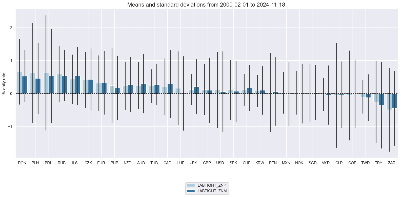
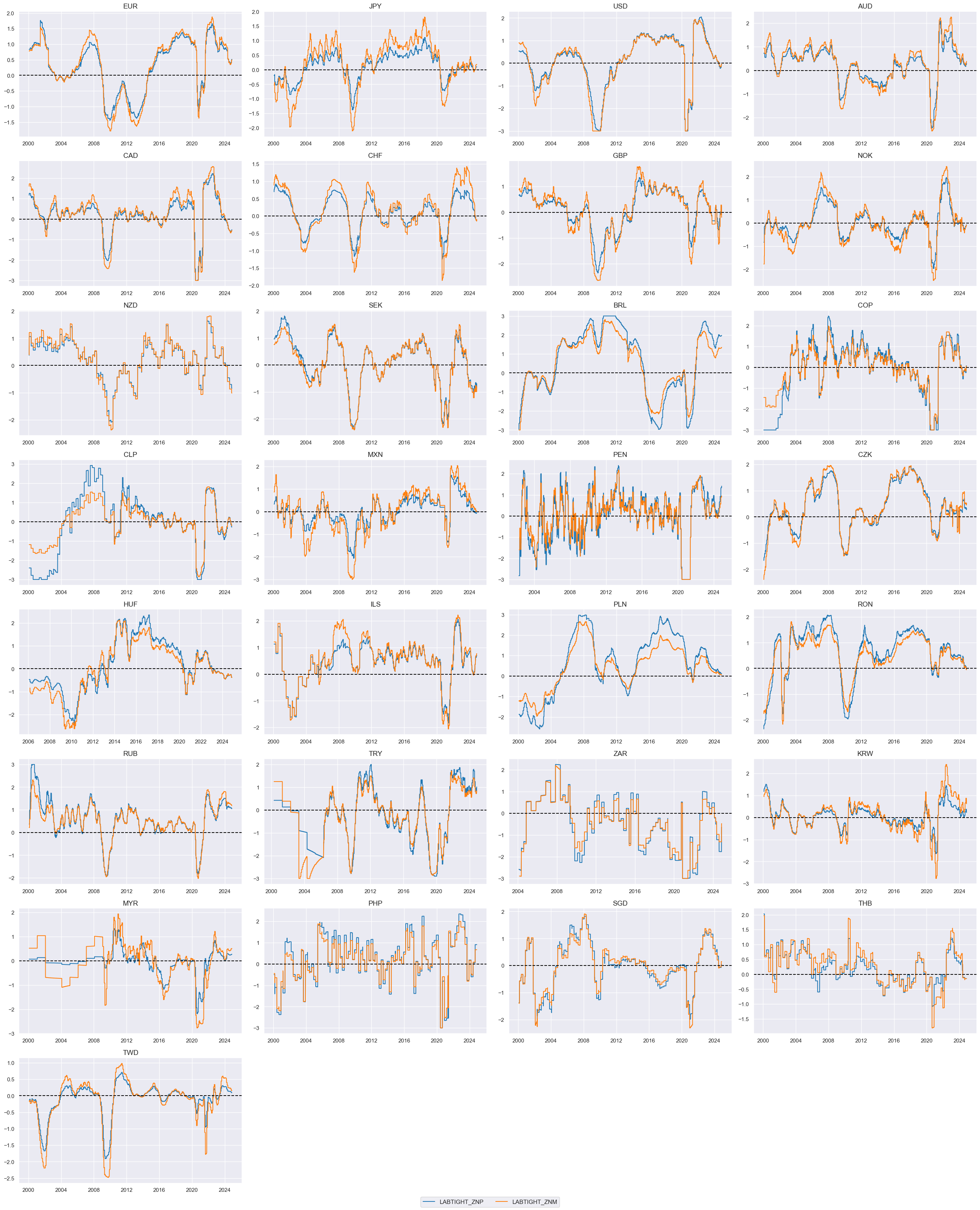
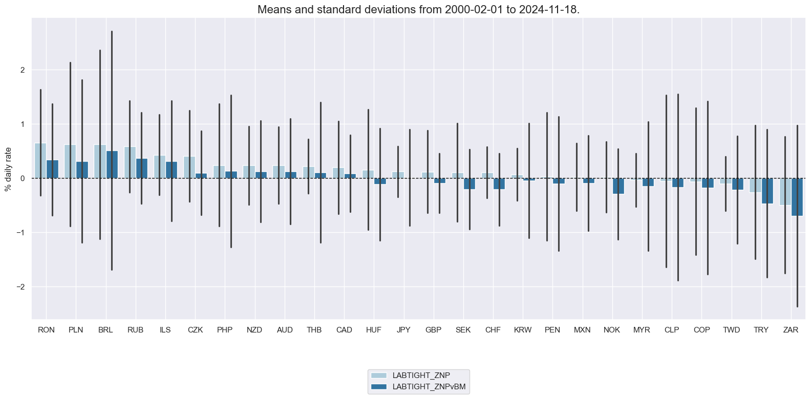
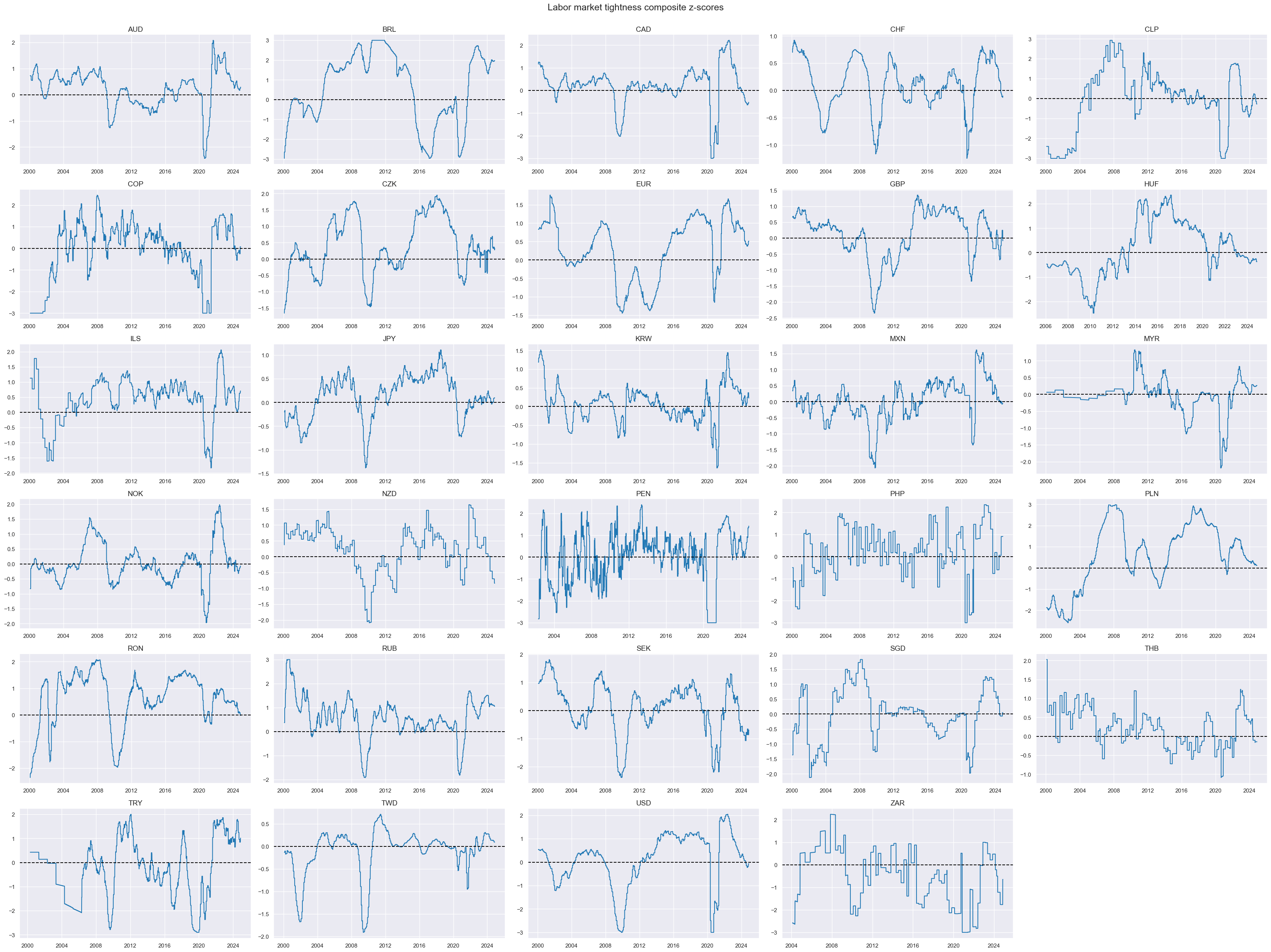
To summarize: we created two Labor market tightening indicators: These are a composite of three quantamental indicators that are jointly tracking the usage of the economy’s labor force. The first is employment growth relative to workforce growth, where the former is measured in % over a year ago and 3-month average and the latter is an estimate based on the latest available 5 years of workforce growth. The second sub-indicator measures changes in the unemployment rate over a year ago and over the last three months, both as a 3-month moving average (view documentation here). The third labor market indicator is the level of the unemployment rate versus a 10-year moving median, again as a 3-month moving average. All three indicators are z-scored, then combined with equal weights, and then the combination is again z-scored for subsequent analysis and aggregation. The difference between the two is the difference in the importance of the panel versus the individual cross-sections for scaling the zn-scores. “_ZNP” indicator uses the whole panel data as the basis for the parameters and “_ZNM” uses 1/4 of the whole panel and 3/4 of an individual cross-section.

xcatx = ["LABTIGHT_ZNP", "LABTIGHT_ZNM"]
cidx = cids

msp.view_ranges(
    dfx,
    cids=cidx,
    xcats=xcatx,
    kind="bar",
    sort_cids_by="mean",
    ylab="% daily rate",
    start="2000-01-01",
)
msp.view_timelines(
    dfx,
    xcats=xcatx,
    cids=cidx,
    ncol=4,
    cumsum=False,
    start="2000-01-01",
    same_y=False,
    size=(12, 12),
    all_xticks=True,
  )

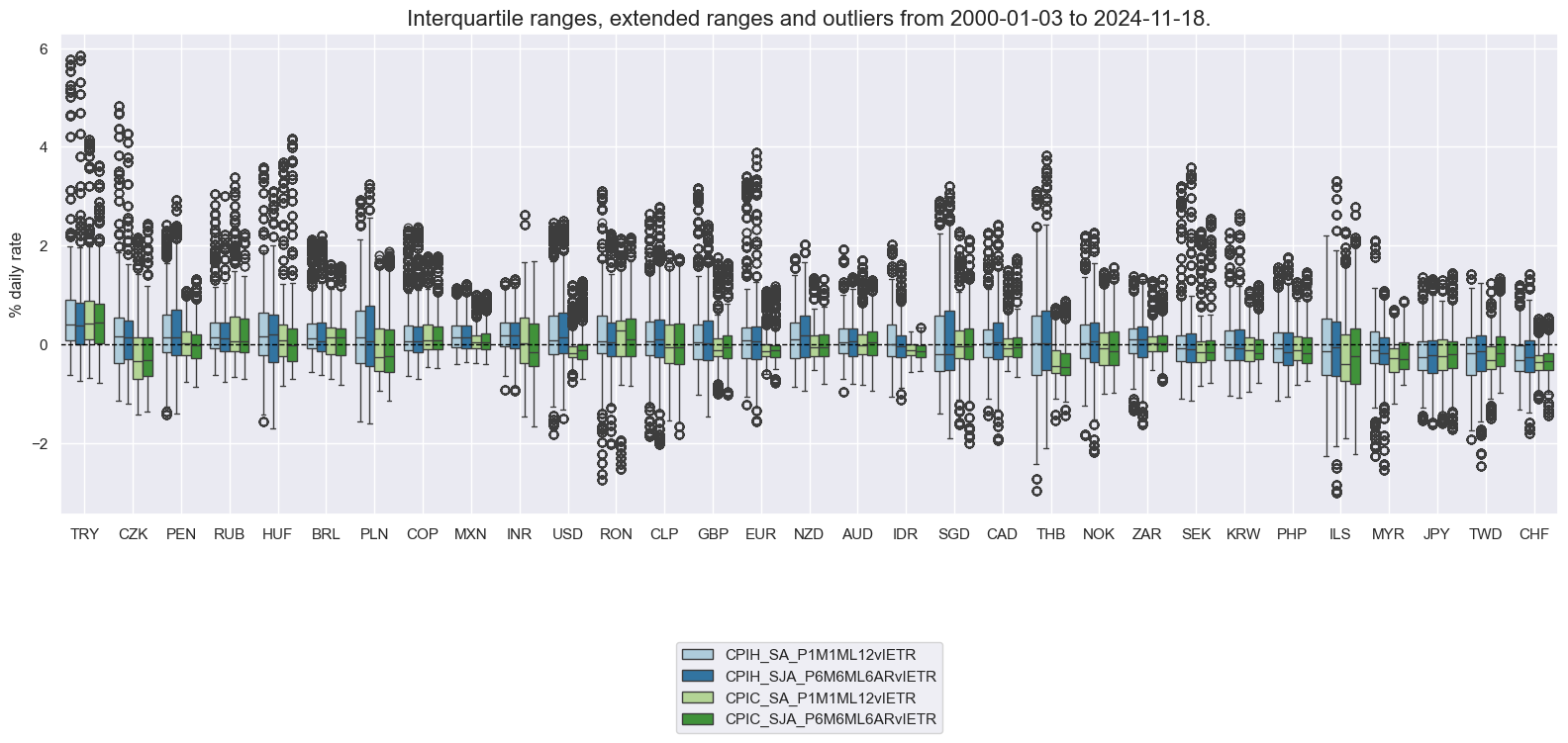
Excess inflation

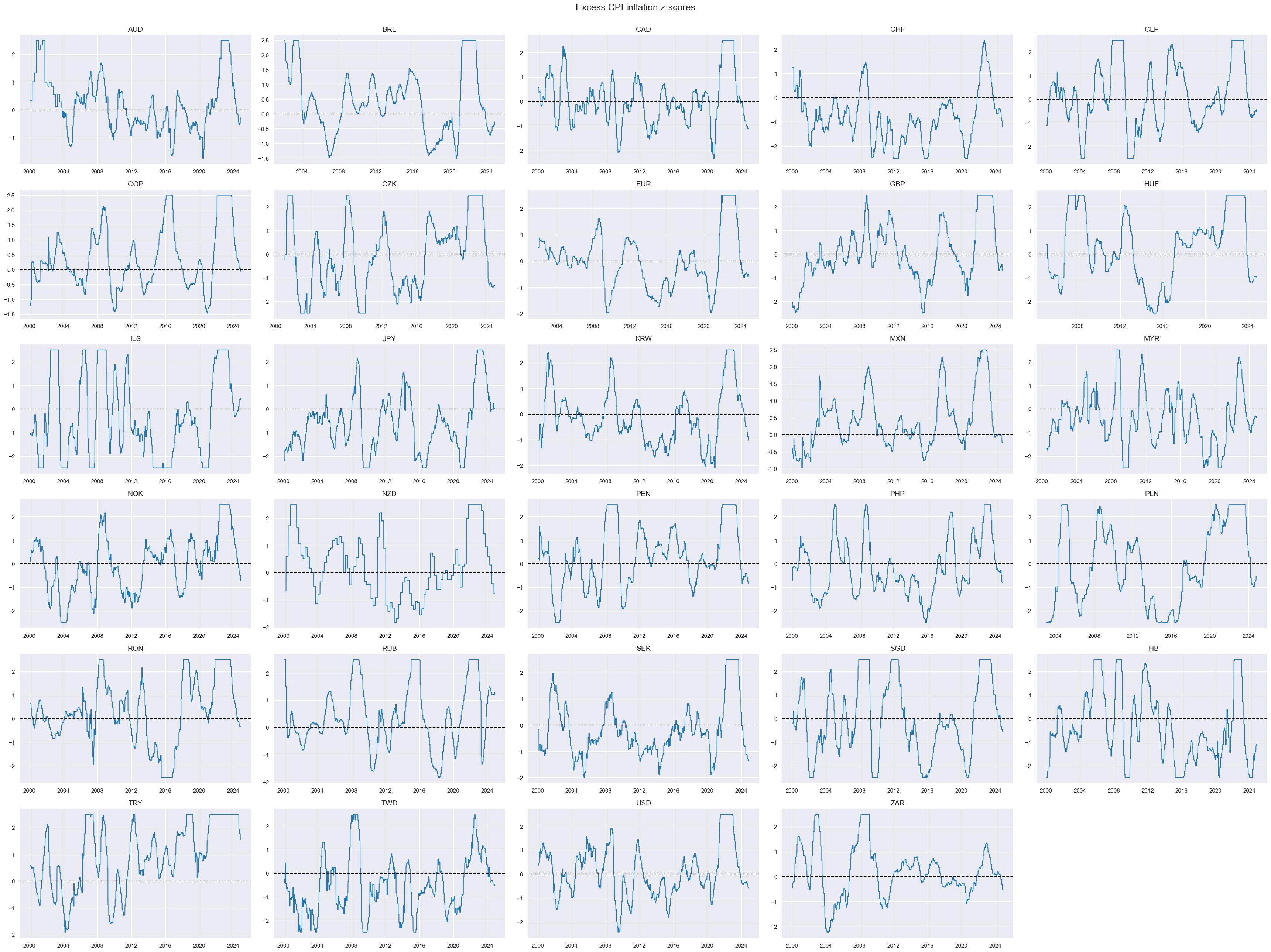
Similarly to labor market tightness, we can calculate plausible metrics of excess inflation versus a country’s effective inflation target. To make the targets comparable across markets, the relative target deviations need denominator bases that should never be less than 2, so we clip the Estimated official inflation target for next year at a minimum value of 2 and use it as denominator. We then calculate absolute and relative target deviations for a range of CPI inflation metrics.

dfa = msp.panel_calculator(
    dfx,
    ["INFTEBASIS = INFTEFF_NSA.clip(lower=2)"],
    cids=cids,
)
dfx = msm.update_df(dfx, dfa)

infs = [
    "CPIH_SA_P1M1ML12",
    "CPIH_SJA_P6M6ML6AR",
    "CPIC_SA_P1M1ML12",
    "CPIC_SJA_P6M6ML6AR",
]

for inf in infs:
    calc_iet = f"{inf}vIETR = ( {inf} - INFTEFF_NSA ) / INFTEBASIS"
    dfa = msp.panel_calculator(dfx, calcs=[calc_iet], cids=cids)
    dfx = msm.update_df(dfx, dfa)

xcatx = [inf + "vIETR" for inf in infs]
cidx = cids

msp.view_ranges(
    dfx,
    cids=cidx,
    xcats=xcatx,
    kind="box",
    sort_cids_by="mean",
    ylab="% daily rate",
    start="2000-01-01",
)
msp.view_timelines(
    dfx,
    xcats=xcatx,
    cids=cidx,
    ncol=4,
    cumsum=False,
    start="2000-01-01",
    same_y=False,
      size=(12, 12),
    all_xticks=True,
  )

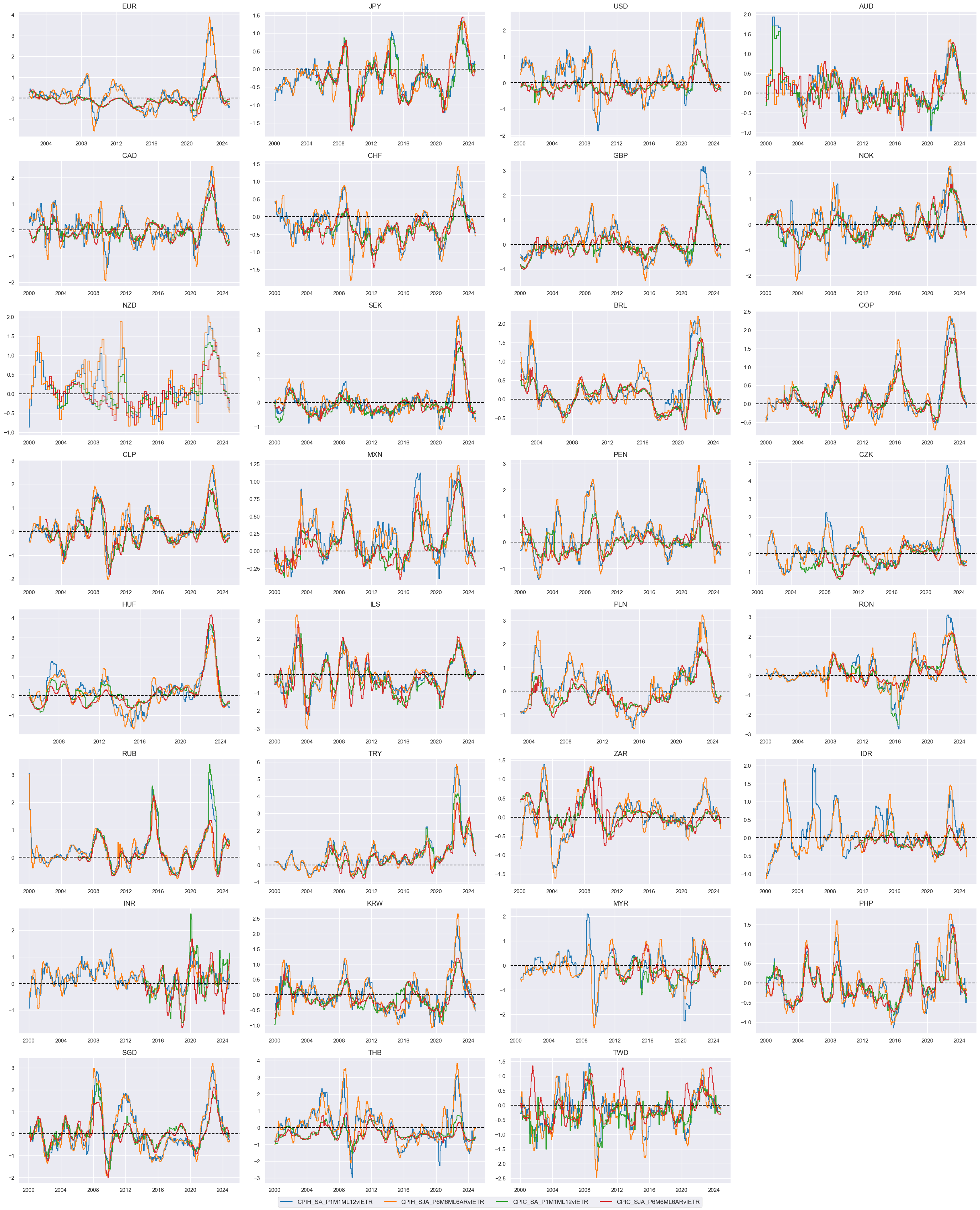
The individual excess inflation metrics are similar in size and, hence can be directly combined into a composite excess inflation metric.

xcatx = [inf + "vIETR" for inf in infs]
cidx = cids

dfa = msp.linear_composite(
    dfx,
    xcats=xcatx,
    cids=cidx,
    complete_xcats=False,  # if some categories are missing the score is based on the remaining
    new_xcat="CPI_PCHvIETR",
)

dfx = msm.update_df(dfx, dfa)

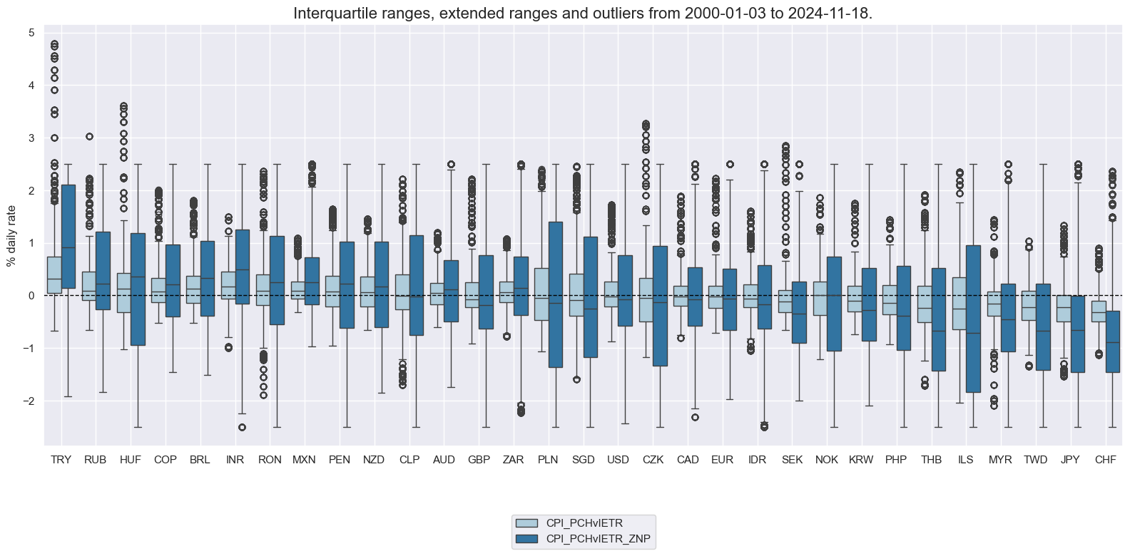
As before, we normalize values for the composite excess inflation metric around zero based on the whole panel.

xcatx = "CPI_PCHvIETR"
cidx = cids

dfa = msp.make_zn_scores(
    dfx,
    xcat=xcatx,
    cids=cidx,
    sequential=True,
    min_obs=522,  # oos scaling after 2 years of panel data
    est_freq="m",
    neutral="zero",
    pan_weight=1,
    thresh=2.5,
    postfix="_ZNP",
)
dfx = msm.update_df(dfx, dfa)

xcatx = ["CPI_PCHvIETR", "CPI_PCHvIETR_ZNP"]
cidx = cids

msp.view_ranges(
    dfx,
    cids=cidx,
    xcats=xcatx,
    kind="box",
    sort_cids_by="mean",
    ylab="% daily rate",
    start="2000-01-01",
)
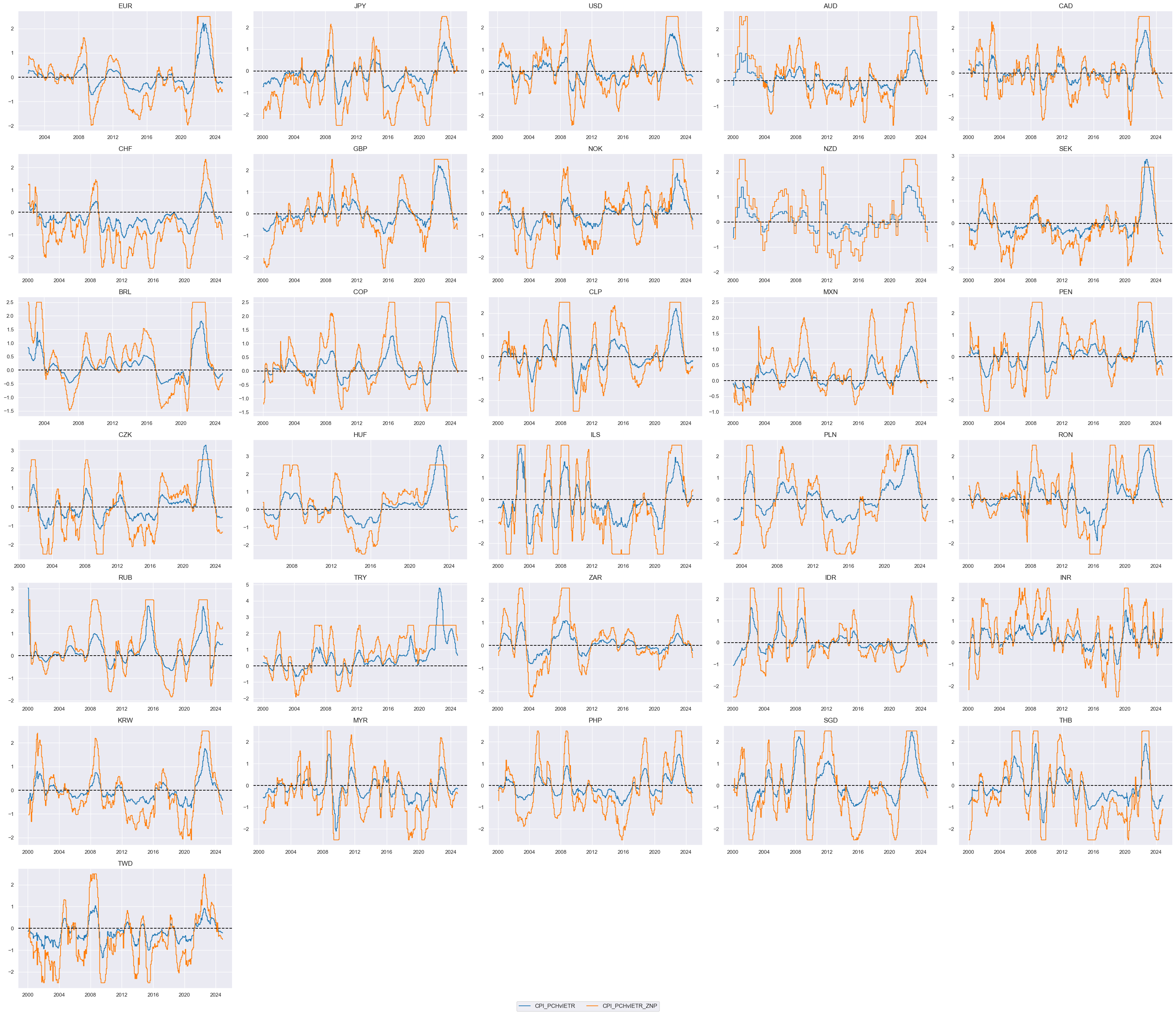
msp.view_timelines(
    dfx,
    xcats=xcatx[0:2],
    cids=cidx,
    ncol=5,
    cumsum=False,
    start="2000-01-01",
    same_y=False,
    size=(12, 12),
    all_xticks=True,
 )

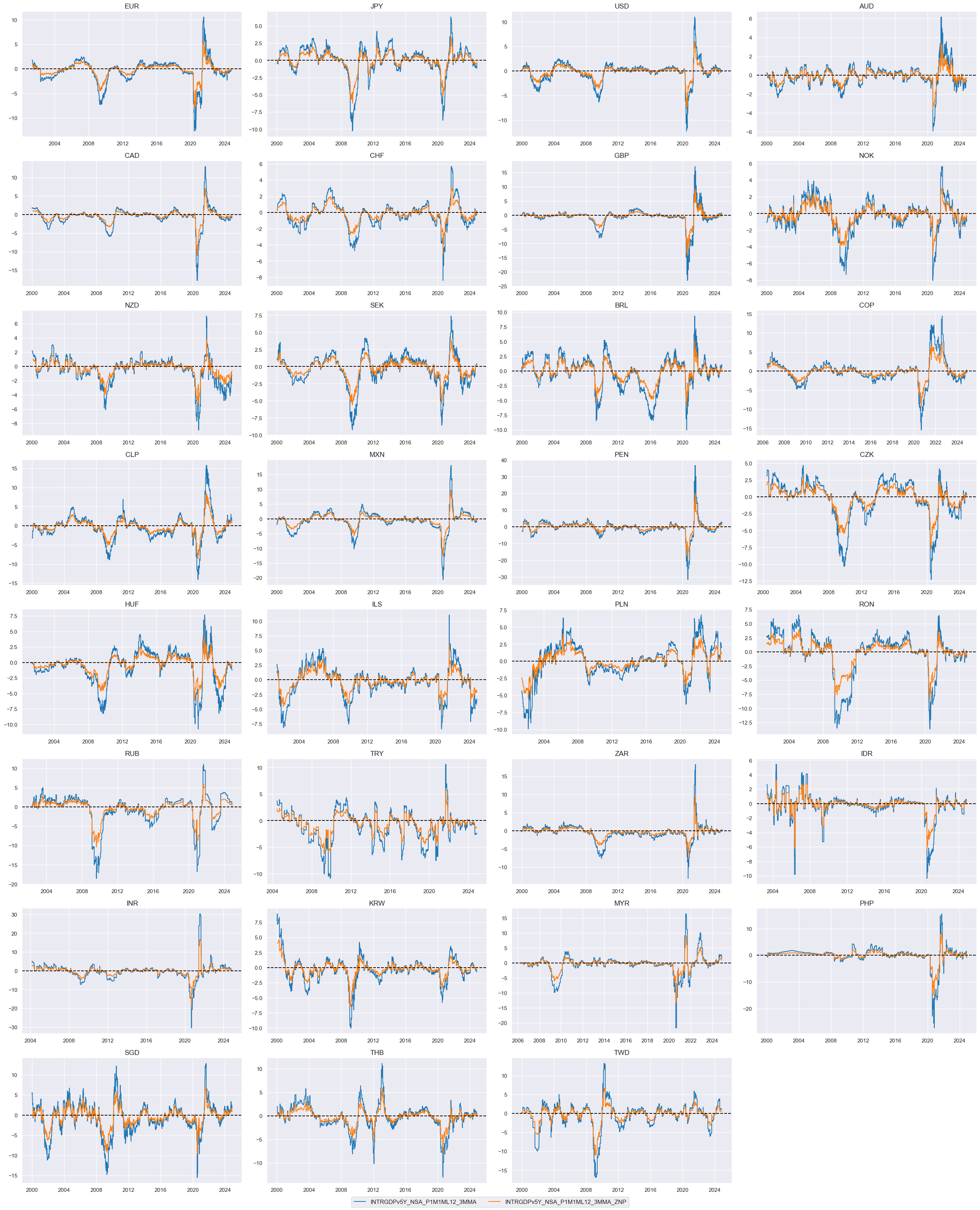
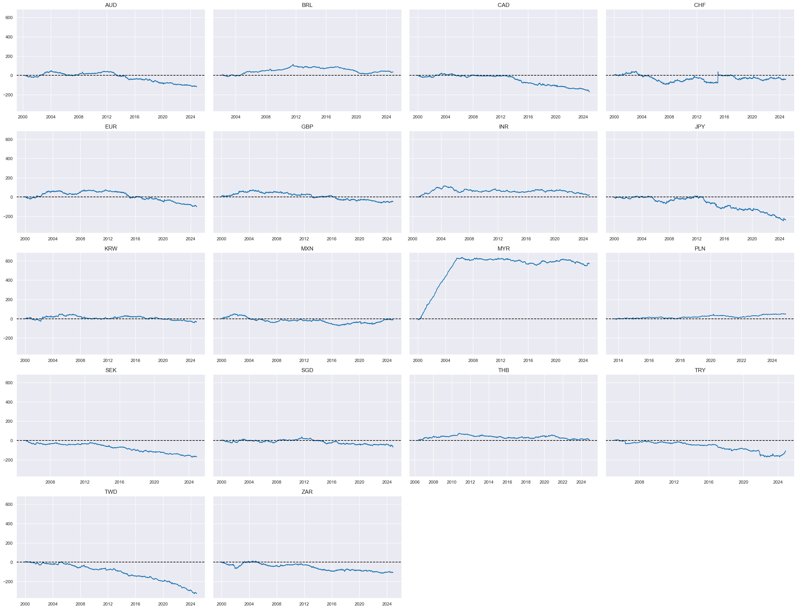
Excess growth

Excess real-time growth estimates are z-scored for intuitive interpretation and to winsorize large outliers, which often reflect temporary disruptions and data issues. JPMaQS offers a ready-made indicator of excess estimated GDP growth trend, labelled INTRGDPv5Y_NSA_P1M1ML12_3MMA . For each day this is the latest estimated GDP growth trend (% over a year ago, 3-month moving average) minus a 5-year median of that country’s actual GDP growth rate. The historic median represents the growth rate that businesses and markets have grown used to. The GDP growth trend is estimated based on actual national accounts and monthly activity data, based on sets of regressions that replicate conventional charting methods in markets (view full documentation here). For subsequent aggregation and analysis, we then z-score the indicator (normalize volatility) around its zero value on an expanding out-of-sample basis using all cross sections for estimating the standard deviations. As before, we normalize values for the indicator around zero based on the whole panel.

xcatx = "INTRGDPv5Y_NSA_P1M1ML12_3MMA"
cidx = cids

dfa = msp.make_zn_scores(
    dfx,
    xcat=xcatx,
    cids=cidx,
    sequential=True,
    min_obs=522,  # oos scaling after 2 years of panel data
    est_freq="m",
    neutral="zero",
    pan_weight=1,
    #  thresh=3,
    postfix="_ZNP",
)
dfx = msm.update_df(dfx, dfa)

xcatx = ["INTRGDPv5Y_NSA_P1M1ML12_3MMA", "INTRGDPv5Y_NSA_P1M1ML12_3MMA_ZNP"]
cidx = cids

msp.view_ranges(
    dfx,
    cids=cidx,
    xcats=xcatx,
    kind="box",
    sort_cids_by="mean",
    ylab="% daily rate",
    start="2000-01-01",
)
msp.view_timelines(
    dfx,
    xcats=xcatx[0:2],
    cids=cidx,
    ncol=4,
    cumsum=False,
    start="2000-01-01",
    same_y=False,
    size=(12, 12),
    all_xticks=True,
 
)

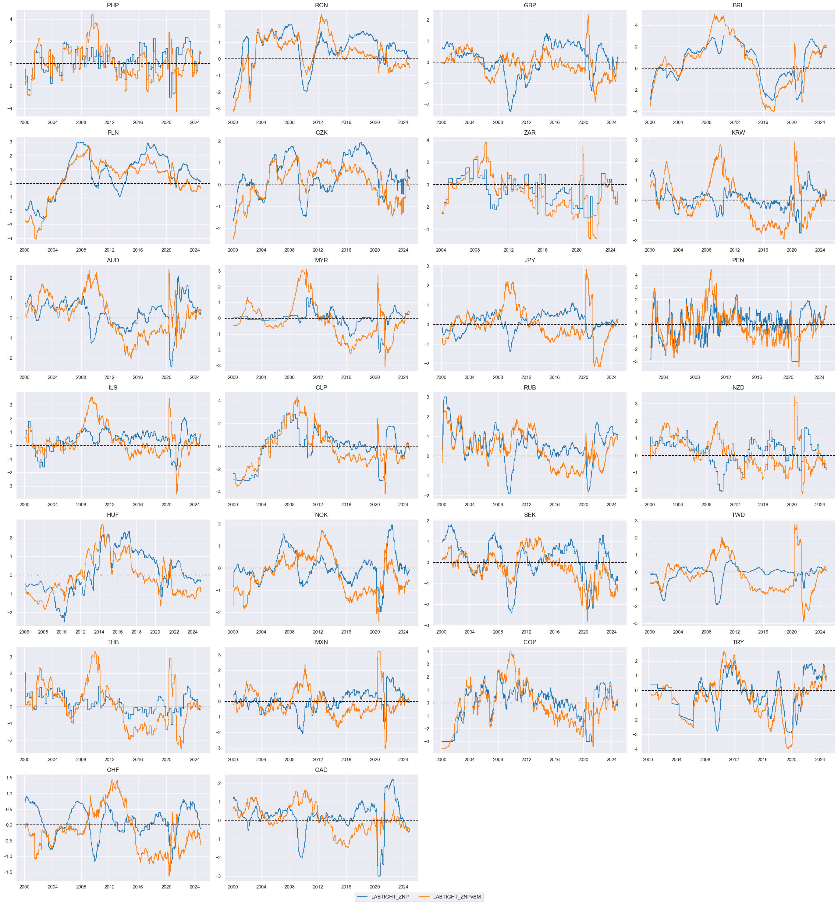
Features relative to the base currency

cycles = [
    "LABTIGHT",
    "CPI_PCHvIETR",
    "INTRGDPv5Y_NSA_P1M1ML12_3MMA",
]
xcatx = [cc + "_ZNP" for cc in cycles]

for xc in xcatx:
    calc_eur = [f"{xc}vBM = {xc} - iEUR_{xc}"]
    calc_usd = [f"{xc}vBM = {xc} - iUSD_{xc}"]
    calc_eud = [f"{xc}vBM = {xc} - 0.5 * ( iEUR_{xc} + iUSD_{xc} )"]

    dfa_eur = msp.panel_calculator(dfx, calcs=calc_eur, cids=cids_eur)
    dfa_usd = msp.panel_calculator(dfx, calcs=calc_usd, cids=cids_usd + ["SGD"])
    dfa_eud = msp.panel_calculator(dfx, calcs=calc_eud, cids=cids_eud)

    dfa = pd.concat([dfa_eur, dfa_usd, dfa_eud])
    dfx = msm.update_df(dfx, dfa)

xcatx = ["LABTIGHT_ZNP", "LABTIGHT_ZNPvBM"]
cidx = cids_fx

msp.view_ranges(
    dfx,
    cids=cidx,
    xcats=xcatx,
    kind="bar",
    sort_cids_by="mean",
    ylab="% daily rate",
    start="2000-01-01",
)
msp.view_timelines(
    dfx,
    xcats=xcatx[0:2],
    cids=cidx,
    ncol=4,
    cumsum=False,
    start="2000-01-01",
    same_y=False,
    size=(12, 12),
    all_xticks=True,
 
)

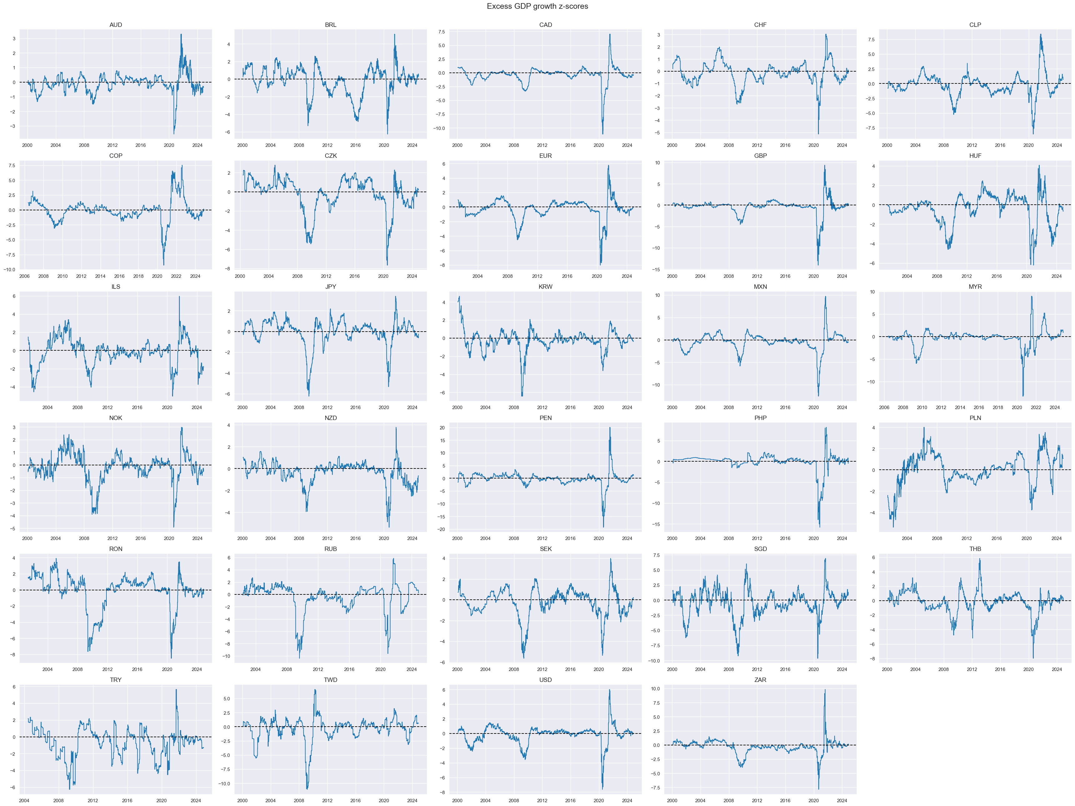
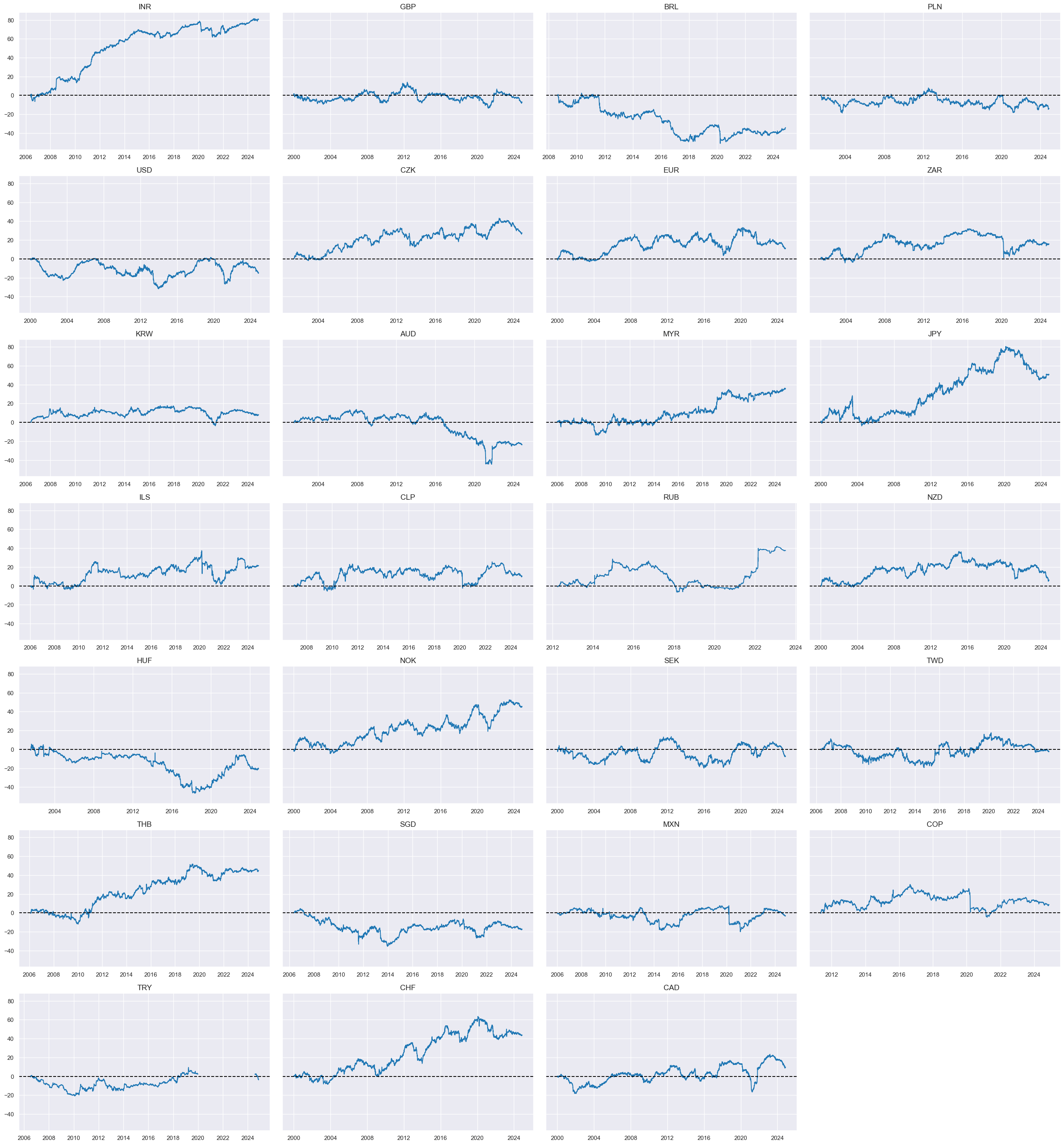
Composite z-scores

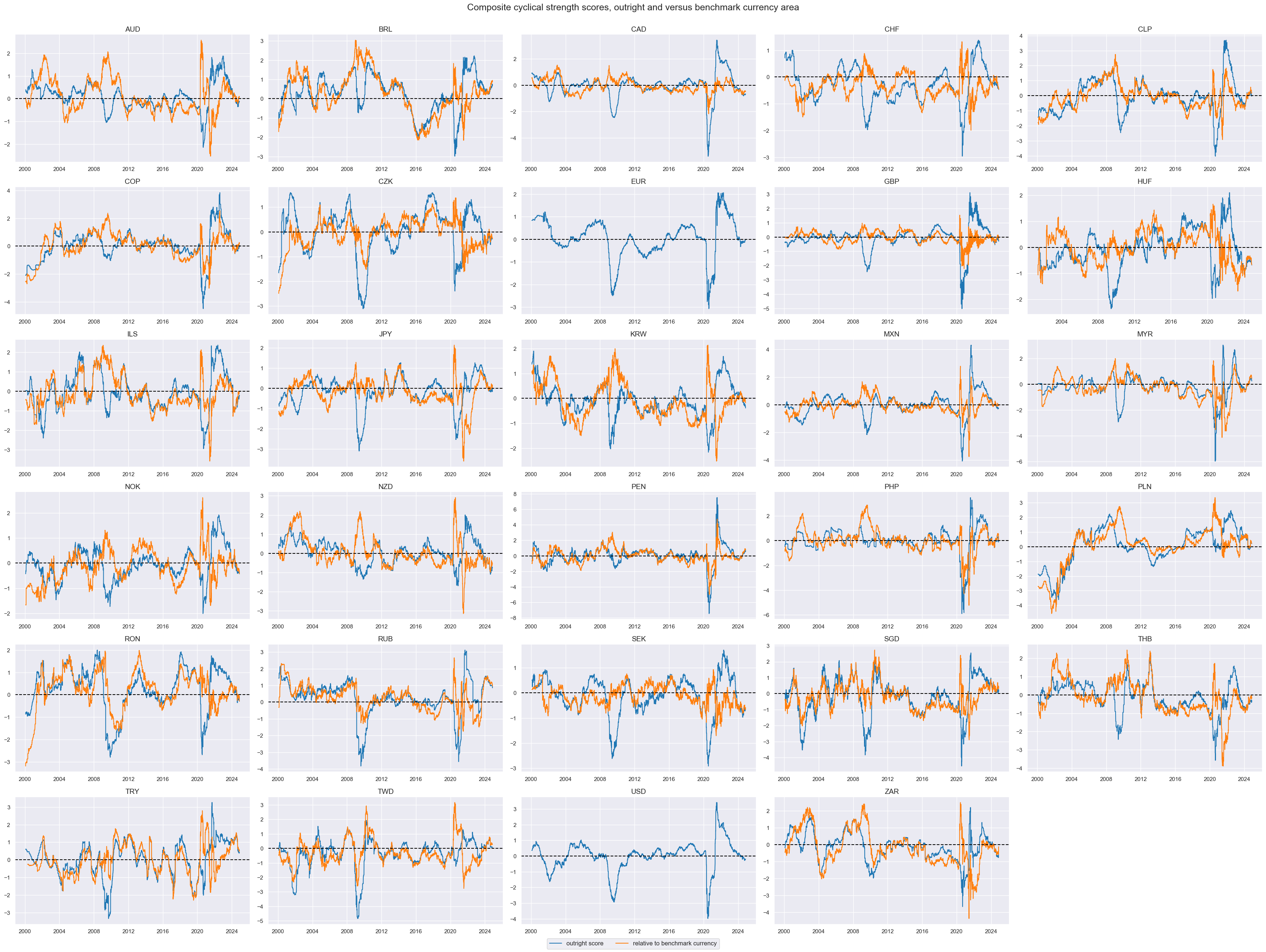
We calculate composite zn-scores of cyclical strength with and without labor market tightness. We also calculate composite zn-score differences to FX base currencies with and without labor market tightness.

# Cyclical strength constituents and list of its keys

d_cs = {
    "G": "INTRGDPv5Y_NSA_P1M1ML12_3MMA",
    "I": "CPI_PCHvIETR",
    "L": "LABTIGHT",
    # "C": "XPCREDITBN_SJA_P1M1ML12",  not so relevant for cyclical strength
}
cs_keys = list(d_cs.keys())


# Available cross-sections

xcatx_znp = [d_cs[i] + "_ZNP" for i in cs_keys]
cidx_znp = msm.common_cids(dfx, xcatx_znp)

xcatx_vbm = [d_cs[i] + "_ZNPvBM" for i in cs_keys]
cidx_vbm = msm.common_cids(dfx, xcatx_vbm)

d_ar = {"_ZNP": cidx_znp, "_ZNPvBM": cidx_vbm}


# Collect all cycle strength key combinations

cs_combs = [combo for r in range(1, 5) for combo in combinations(cs_keys, r)]


# Use key combinations to calculate all possible factor combinations

dfa = pd.DataFrame(columns=dfx.columns).reindex([])

for cs in cs_combs:
    for key, value in d_ar.items():
        xcatx = [
            d_cs[i] + key for i in cs
        ]  # extract absolute or relative xcat combination
        dfaa = msp.linear_composite(
            dfx,
            xcats=xcatx,
            cids=value,
            complete_xcats=False,  # if some categories are missing the score is based on the remaining
            new_xcat="CS" + "".join(cs) + key[4:] + "_ZC",
        )
        dfa = msm.update_df(dfa, dfaa)

dfx = msm.update_df(dfx, dfa)


# Collect factor combinations in lists

cs_all = dfa["xcat"].unique()
cs_dir = [cs for cs in cs_all if "vBM" not in cs]
cs_rel = [cs for cs in cs_all if "vBM" in cs]

xcatx = ["CSG_ZC"]
cidx = cidx_znp

msp.view_timelines(
    dfx,
    xcats=xcatx[0:2],
    cids=cidx,
    ncol=5,
    cumsum=False,
    start="2000-01-01",
    same_y=False,
    size=(12, 12),
    all_xticks=True,
    title="Excess GDP growth z-scores",
)

xcatx = ["CSL_ZC"]
cidx = cidx_znp

msp.view_timelines(
    dfx,
    xcats=xcatx[0:2],
    cids=cidx,
    ncol=5,
    cumsum=False,
    start="2000-01-01",
    same_y=False,
    size=(12, 12),
    all_xticks=True,
    title="Labor market tightness composite z-scores",
  
)

xcatx = ["CSI_ZC"]
cidx = cidx_znp

msp.view_timelines(
    dfx,
    xcats=xcatx[0:2],
    cids=cidx,
    ncol=5,
    cumsum=False,
    start="2000-01-01",
    same_y=False,
     size=(12, 12),
    all_xticks=True,
    title="Excess CPI inflation z-scores",
  )

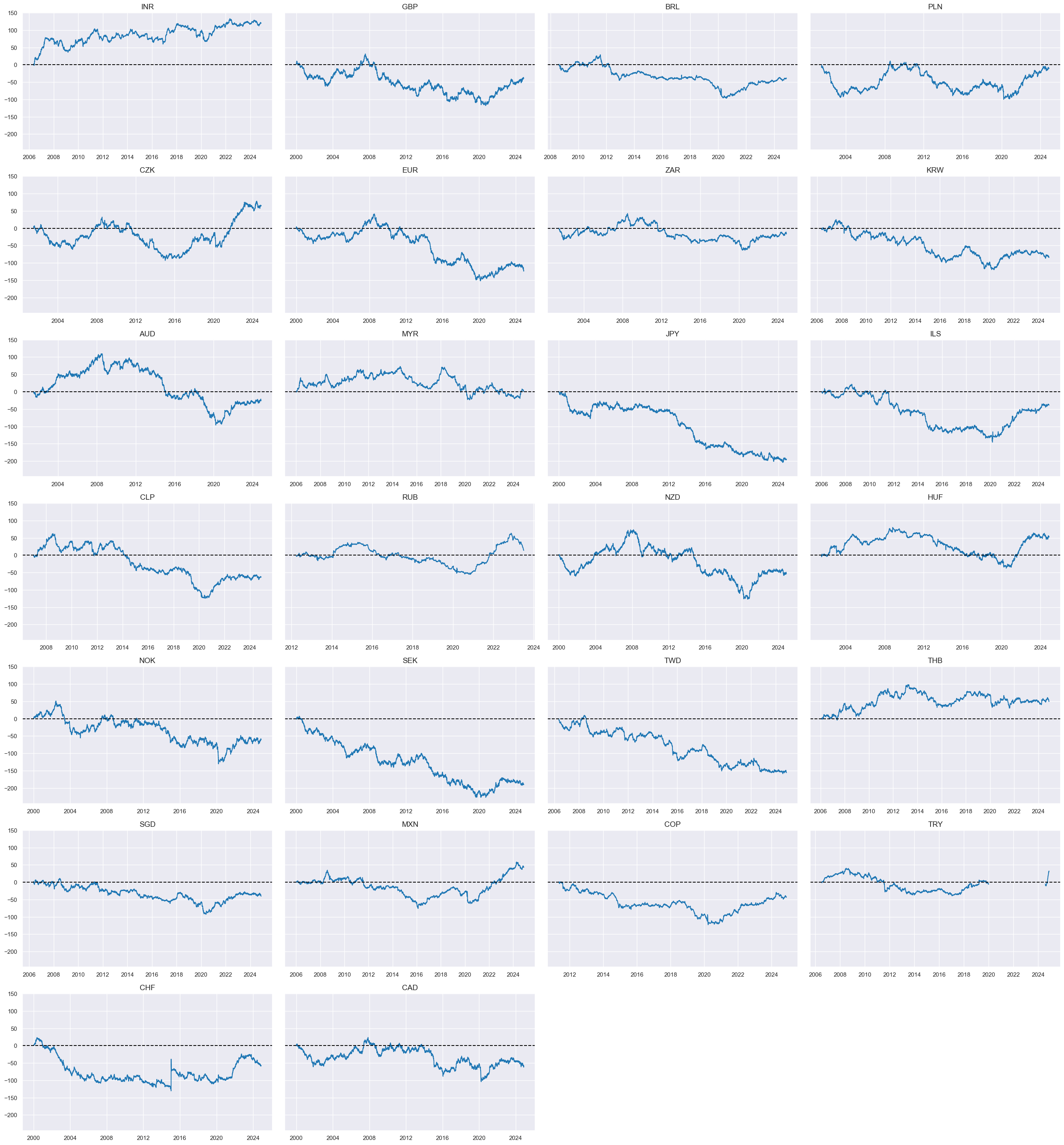
xcatx = ["CSGIL_ZC", "CSGILvBM_ZC"]
cidx = cidx_znp

msp.view_timelines(
    dfx,
    xcats=xcatx[0:2],
    xcat_labels=["outright score", "relative to benchmark currency"],
    cids=cidx,
    ncol=5,
    cumsum=False,
    start="2000-01-01",
    same_y=False,
    size=(12, 12),
    all_xticks=True,
    title="Composite cyclical strength scores, outright and versus benchmark currency area",
   )

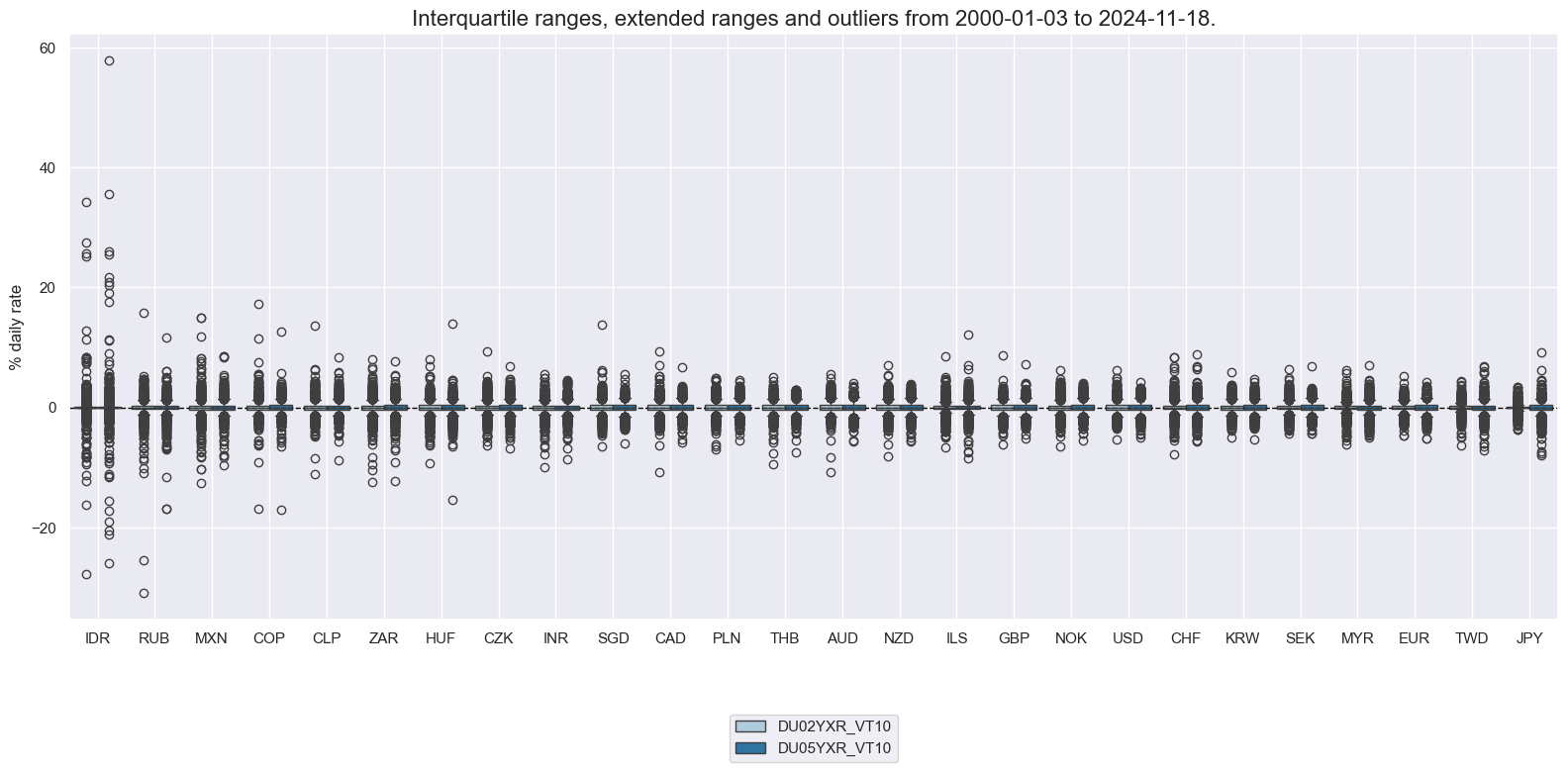
Targets

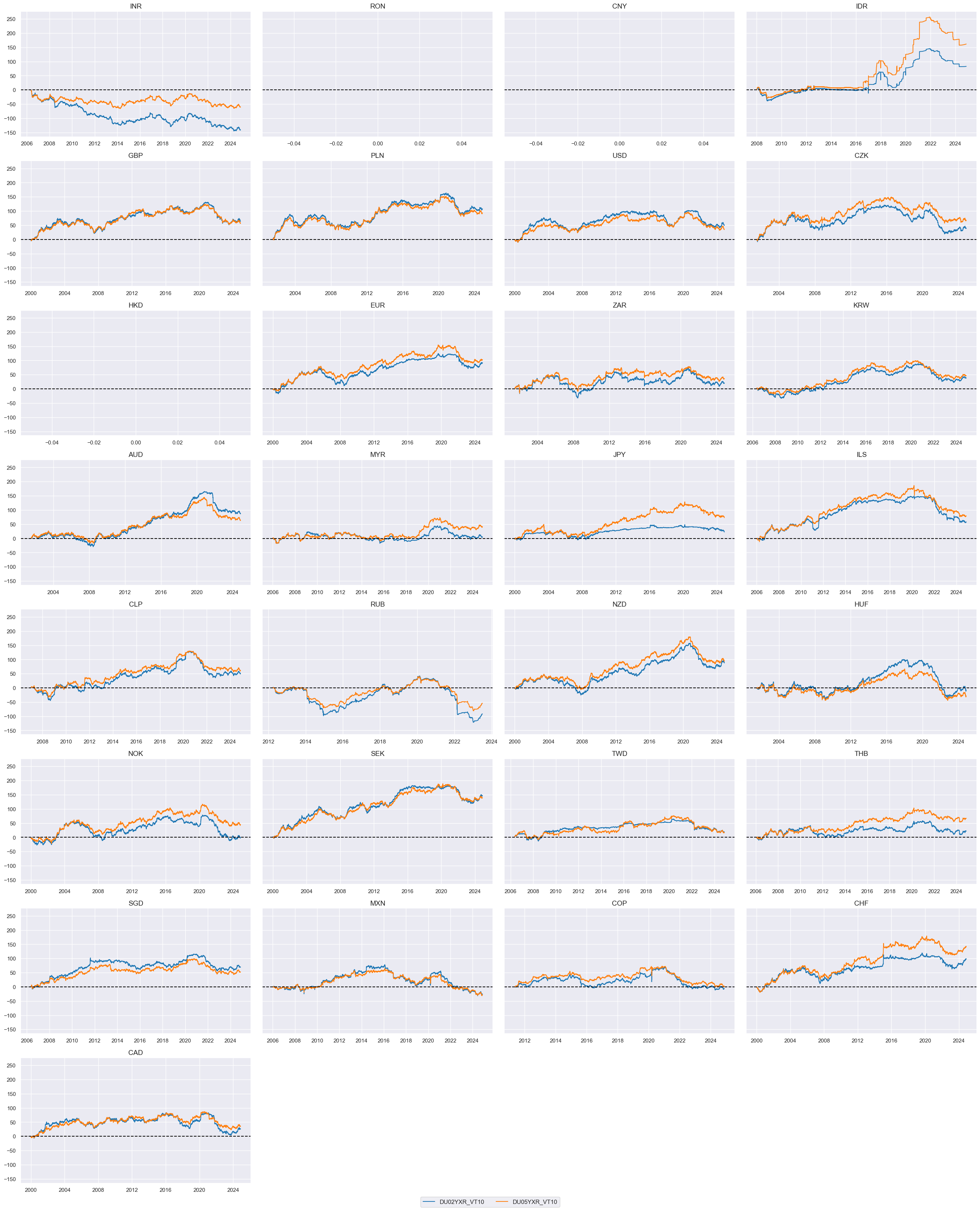
Directional vol-targeted IRS returns

xcatx = ["DU02YXR_VT10", "DU05YXR_VT10"]
cidx = list(set(cids_du) - set(["TRY"]))


msp.view_ranges(
    dfx,
    cids=cidx,
    xcats=xcatx,
    kind="box",
    sort_cids_by="std",
    ylab="% daily rate",
    start="2000-01-01",
)

msp.view_timelines(
    dfx,
    xcats=xcatx,
    cids=cidx,
    ncol=4,
    cumsum=True,
    start="2000-01-01",
    same_y=True,
    size=(12, 12),
    all_xticks=True,
  )

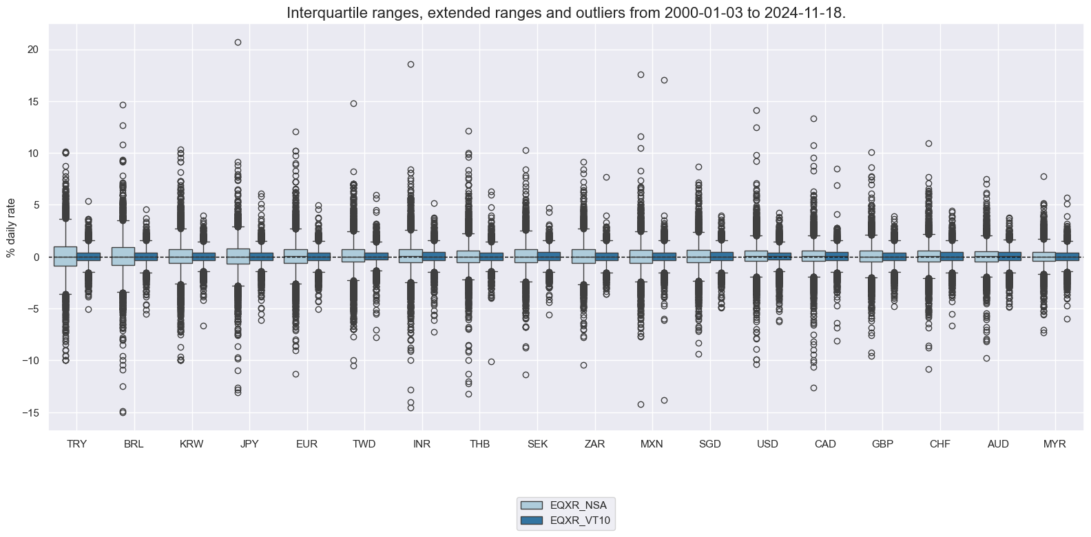
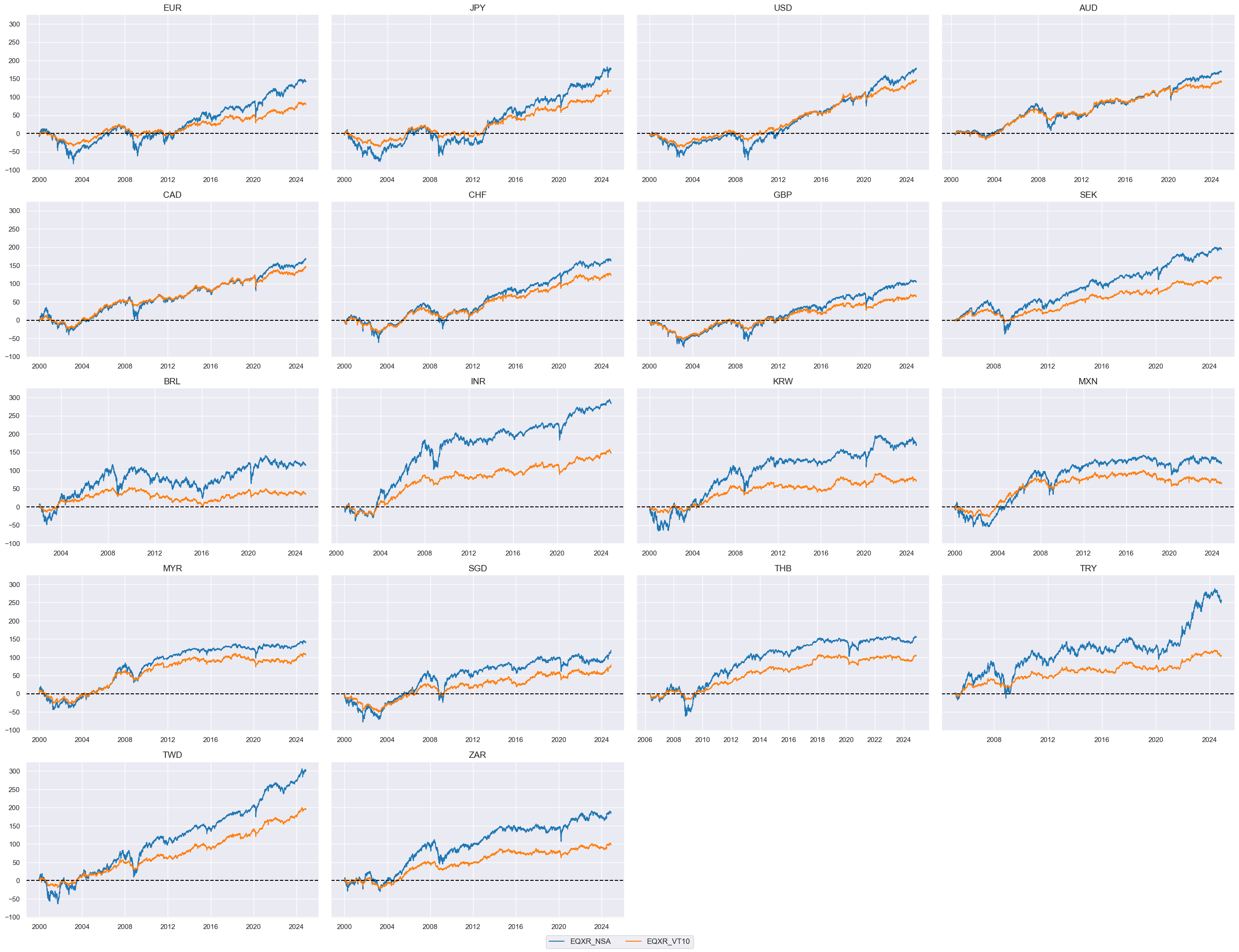
Directional equity returns

xcatx = ["EQXR_NSA", "EQXR_VT10"]
cidx = cids_eq

msp.view_ranges(
    dfx,
    cids=cidx,
    xcats=xcatx,
    kind="box",
    sort_cids_by="std",
    ylab="% daily rate",
    start="2000-01-01",
)

msp.view_timelines(
    dfx,
    xcats=xcatx,
    cids=cidx,
    ncol=4,
    cumsum=True,
    start="2000-01-01",
    same_y=True,
    size=(12, 12),
    all_xticks=True,
 
)

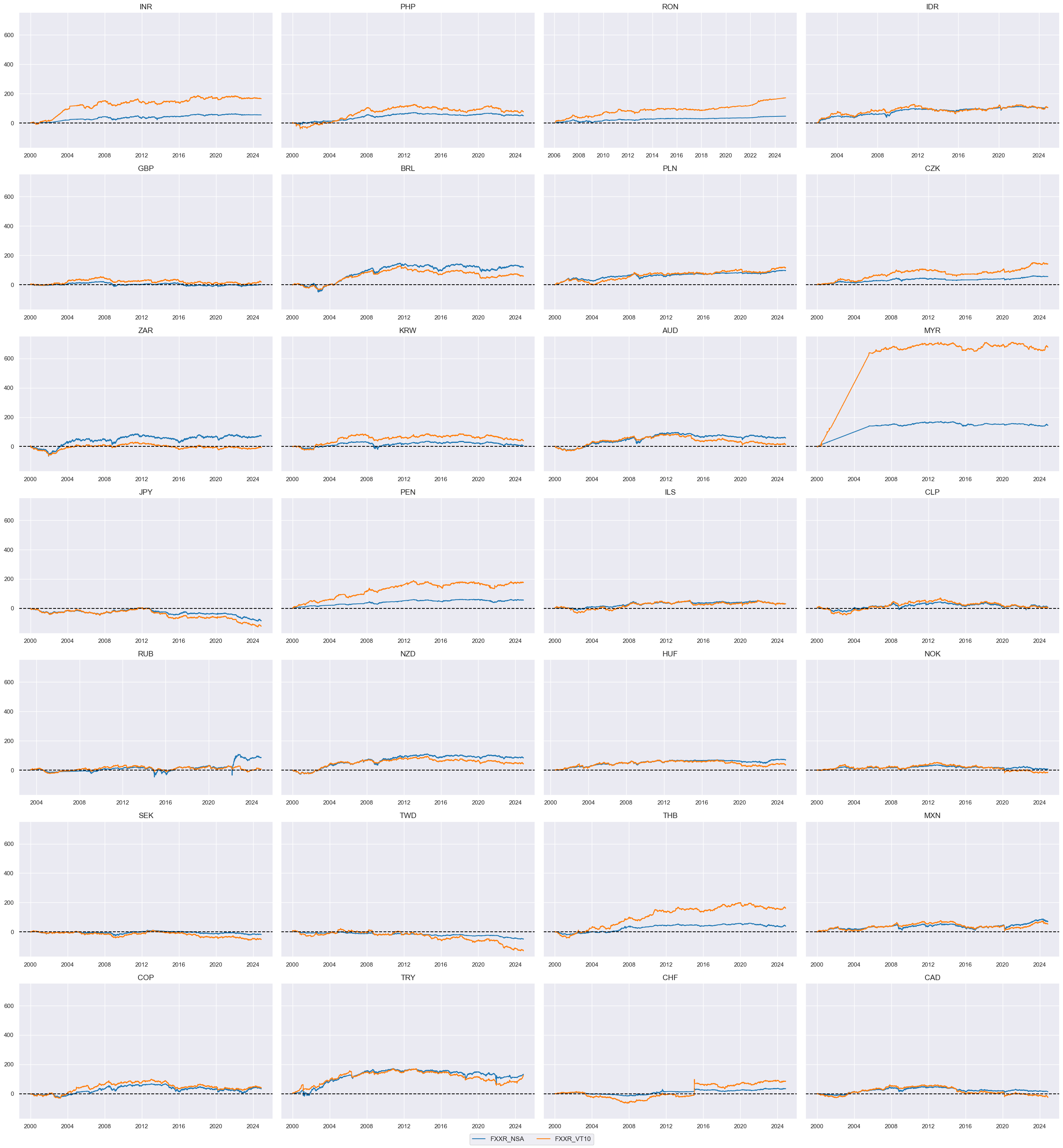
FX returns relative to base currencies

xcatx = ["FXXR_NSA", "FXXR_VT10"]
cidx = cids_fx

msp.view_timelines(
    dfx,
    xcats=xcatx,
    cids=cidx,
    ncol=4,
    cumsum=True,
    start="2000-01-01",
    same_y=True,
    size=(12, 12),
    all_xticks=True,
  
)

FX versus equity returns

cidx_fxeq = msm.common_cids(dfx, ["FXXR_VT10", "EQXR_VT10"])
calcs = ["FXvEQXR = FXXR_VT10 - EQXR_VT10 "]
dfa = msp.panel_calculator(dfx, calcs=calcs, cids=cidx_fxeq, blacklist=None)
dfx = msm.update_df(dfx, dfa)

xcatx = ["FXvEQXR"]
cidx = cidx_fxeq

msp.view_timelines(
    dfx,
    xcats=xcatx,
    cids=cidx,
    ncol=4,
    cumsum=True,
    start="2000-01-01",
    same_y=True,
    size=(12, 12),
    all_xticks=True,
)

FX versus IRS returns

cidx_fxdu = list(
    set(msm.common_cids(dfx, ["FXXR_VT10", "DU05YXR_VT10"])) - set(["IDR"])
)
calcs = ["FXvDU05XR = FXXR_VT10 - DU05YXR_VT10 "]
dfa = msp.panel_calculator(dfx, calcs=calcs, cids=cidx_fxdu, blacklist=dublack)
dfx = msm.update_df(dfx, dfa)

xcatx = ["FXvDU05XR"]
cidx = cidx_fxdu

msp.view_timelines(
    dfx,
    xcats=xcatx,
    cids=cidx,
    ncol=4,
    cumsum=True,
    start="2000-01-01",
    same_y=True,
    size=(12, 12),
    all_xticks=True,
 
)

2s-5s flattener returns

cidx_du52 = list(
    set(msm.common_cids(dfx, ["DU02YXR_VT10", "DU05YXR_VT10"])) - set(["IDR"])
)
calcs = ["DU05v02XR = DU05YXR_VT10 - DU02YXR_VT10 "]
dfa = msp.panel_calculator(dfx, calcs=calcs, cids=cidx_du52, blacklist=dublack)
dfx = msm.update_df(dfx, dfa)

xcatx = ["DU05v02XR"]
cidx = cidx_du52

msp.view_timelines(
    dfx,
    xcats=xcatx,
    cids=cidx,
    ncol=4,
    cumsum=True,
    start="2000-01-01",
    same_y=True,
    size=(12, 12),
    all_xticks=True,
  
)

Value checks

Directional equity strategy

Specs and panel test

sigs = cs_dir
ms = "CSGIL_ZC"  # main signal
oths = list(set(sigs) - set([ms]))  # other signals

targ = "EQXR_VT10"
cidx = msm.common_cids(dfx, sigs + [targ])
# cidx = list(set(cids_dm) & set(cidx))   # for DM alone

dict_eqdi = {
    "sig": ms,
    "rivs": oths,
    "targ": targ,
    "cidx": cidx,
    "black": fxblack,
    "srr": None,
    "pnls": None,
}

dix = dict_eqdi

sig = dix["sig"]
targ = dix["targ"]
cidx = dix["cidx"]
blax = dix["black"]

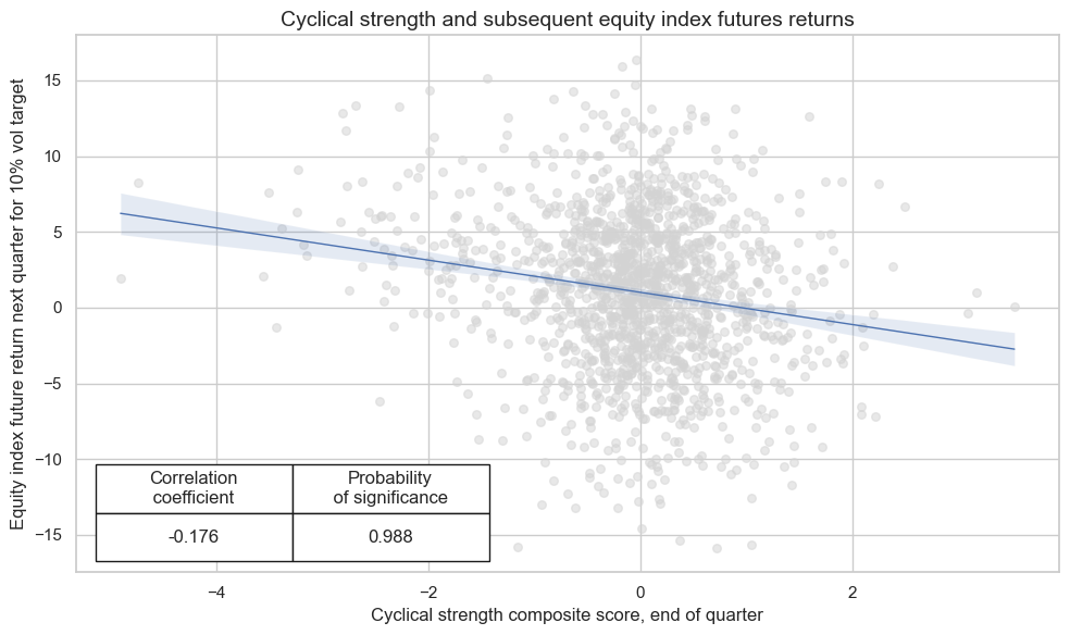
crx = msp.CategoryRelations(
    dfx,
    xcats=[sig, targ],
    cids=cidx,
    freq="Q",  # quarterly frequency allows for policy inertia
    lag=1,
    xcat_aggs=["last", "sum"],
    start="2000-01-01",
    blacklist=blax,
    xcat_trims=[None, None],
)
crx.reg_scatter(
    labels=False,
    coef_box="lower left",
    xlab="Cyclical strength composite score, end of quarter",
    ylab="Equity index future return next quarter for 10% vol target",
    title="Cyclical strength and subsequent equity index futures returns",
    size=(10, 6),
    prob_est="map",
)

Accuracy and correlation check

dix = dict_eqdi

sig = dix["sig"]
rivs = dix["rivs"]
targ = dix["targ"]
cidx = dix["cidx"]
blax = dix["black"]

srr = mss.SignalReturnRelations(
    dfx,
    cids=cidx,
    sigs=[sig] + rivs,
    sig_neg=[True] + [True] * len(rivs),
    rets=targ,
    freqs="M",
    start="2000-01-01",
    blacklist=blax,
)

dix["srr"] = srr

dix = dict_eqdi
srrx = dix["srr"]
display(srrx.summary_table().astype("float").round(3))

	accuracy	bal_accuracy	pos_sigr	pos_retr	pos_prec	neg_prec	pearson	pearson_pval	kendall	kendall_pval	auc
M: CSGIL_ZC_NEG/last => EQXR_VT10	0.523	0.522	0.506	0.586	0.608	0.437	0.100	0.000	0.053	0.000	0.523
Mean years	0.522	0.511	0.502	0.583	0.592	0.430	0.043	0.450	0.025	0.435	0.508
Positive ratio	0.600	0.560	0.600	0.680	0.800	0.280	0.600	0.360	0.600	0.400	0.560
Mean cids	0.522	0.519	0.505	0.583	0.600	0.437	0.100	0.227	0.051	0.308	0.519
Positive ratio	0.824	0.706	0.471	0.941	0.941	0.059	0.941	0.824	0.765	0.647	0.706

dix = dict_eqdi
srrx = dix["srr"]
display(srrx.signals_table().sort_index().astype("float").round(3))

				accuracy	bal_accuracy	pos_sigr	pos_retr	pos_prec	neg_prec	pearson	pearson_pval	kendall	kendall_pval	auc
Return	Signal	Frequency	Aggregation
EQXR_VT10	CSGIL_ZC_NEG	M	last	0.523	0.522	0.506	0.586	0.608	0.437	0.100	0.000	0.053	0.000	0.523
	CSGI_ZC_NEG	M	last	0.535	0.525	0.555	0.586	0.609	0.442	0.087	0.000	0.048	0.000	0.526
	CSGL_ZC_NEG	M	last	0.492	0.501	0.448	0.586	0.587	0.415	0.075	0.000	0.032	0.002	0.501
	CSG_ZC_NEG	M	last	0.515	0.508	0.538	0.586	0.593	0.423	0.051	0.001	0.014	0.171	0.508
	CSIL_ZC_NEG	M	last	0.527	0.528	0.495	0.586	0.614	0.442	0.108	0.000	0.063	0.000	0.529
	CSI_ZC_NEG	M	last	0.538	0.529	0.551	0.586	0.612	0.446	0.084	0.000	0.049	0.000	0.530
	CSL_ZC_NEG	M	last	0.496	0.515	0.396	0.586	0.604	0.425	0.082	0.000	0.046	0.000	0.514

dix = dict_eqdi
srrx = dix["srr"]
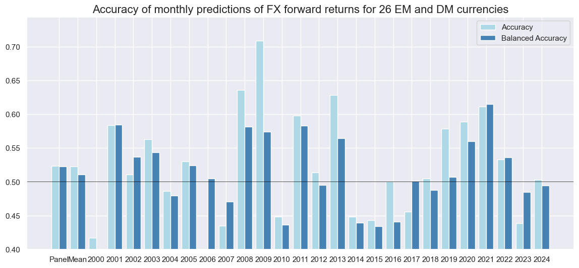
srrx.accuracy_bars(
    type="years",
    title="Accuracy of monthly predictions of FX forward returns for 26 EM and DM currencies",
    size=(14, 6),
)

Naive PnL

dix = dict_eqdi

sigx = [dix["sig"]] + dix["rivs"]
targ = dix["targ"]
cidx = dix["cidx"]
blax = dix["black"]

naive_pnl = msn.NaivePnL(
    dfx,
    ret=targ,
    sigs=sigx,
    cids=cidx,
    start="2000-01-01",
    blacklist=blax,
    bms=["USD_EQXR_NSA"],
)

for sig in sigx:
    naive_pnl.make_pnl(
        sig,
        sig_neg=True,
        sig_op="zn_score_pan",
        thresh=3,
        rebal_freq="monthly",
        vol_scale=10,
        rebal_slip=1,
        pnl_name=sig + "_PZN",
    )

for sig in sigx:
    naive_pnl.make_pnl(
        sig,
        sig_neg=True,
        sig_op="binary",
        thresh=3,
        rebal_freq="monthly",
        vol_scale=10,
        rebal_slip=1,
        pnl_name=sig + "_BIN",
    )

naive_pnl.make_long_pnl(vol_scale=10, label="Long only")
dix["pnls"] = naive_pnl

dix = dict_eqdi

sigx = dix["sig"]
naive_pnl = dix["pnls"]
pnls = [sigx + x for x in ["_PZN", "_BIN"]] + ["Long only"]

naive_pnl.plot_pnls(
    pnl_cats=pnls,
    pnl_cids=["ALL"],
    start="2000-01-01",
    title=None,
    xcat_labels=None,
    figsize=(16, 8),
)

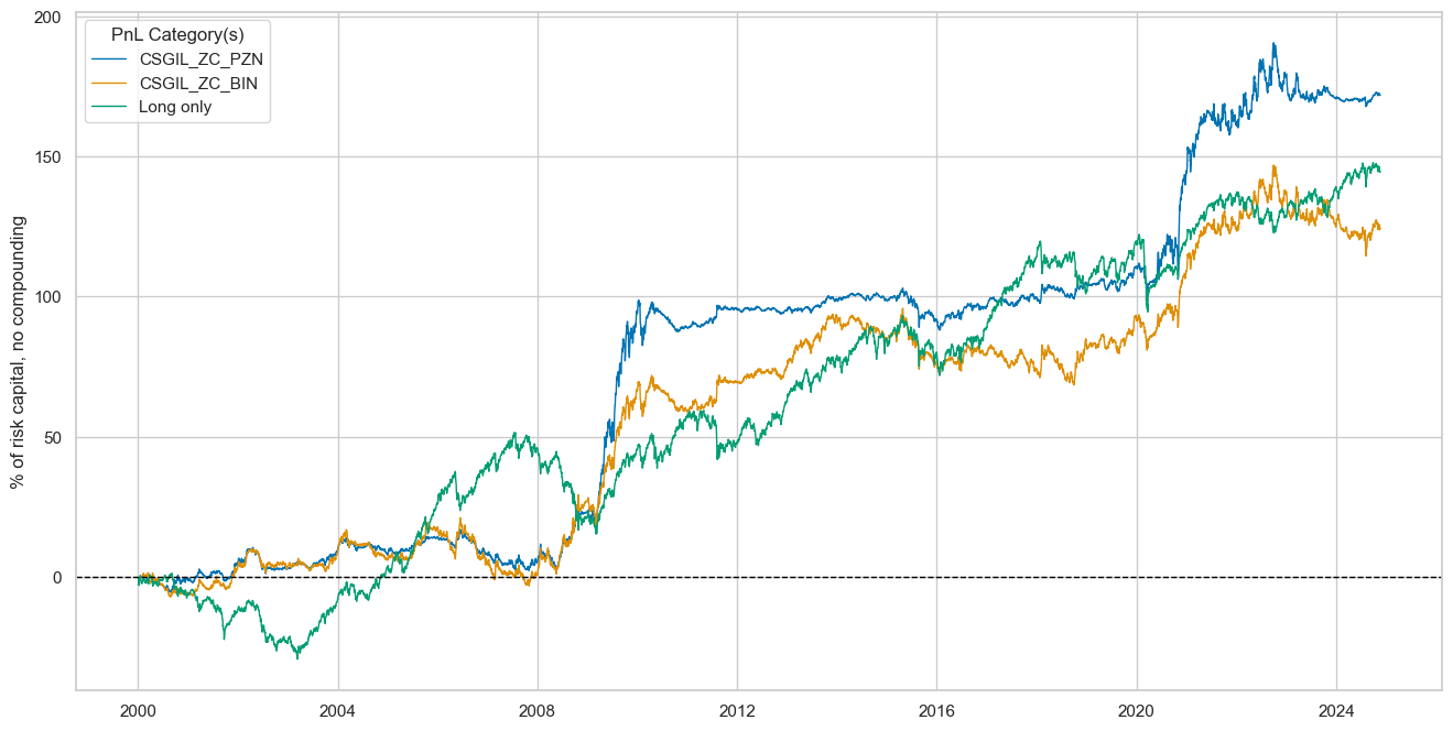
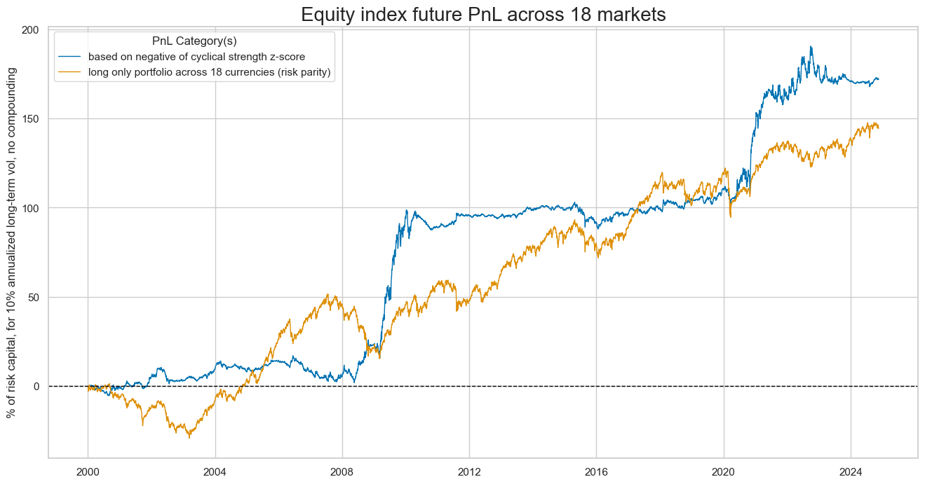
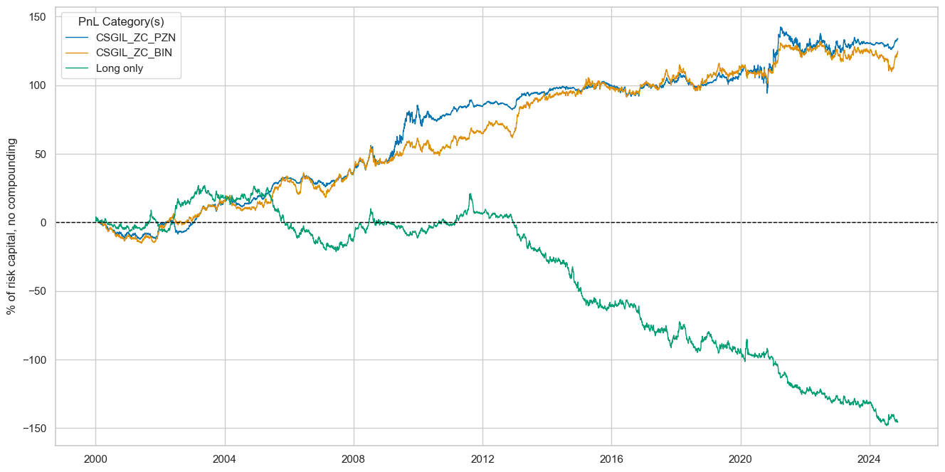
dix = dict_eqdi

sigx = dix["sig"]
naive_pnl = dix["pnls"]
pnls = [sigx + "_PZN"] + ["Long only"]

dict_labels={"CSGIL_ZC_PZN": "based on negative of cyclical strength z-score",
            "Long only": "long only portfolio across 18 currencies (risk parity)"}

naive_pnl.plot_pnls(
    pnl_cats=pnls,
    pnl_cids=["ALL"],
    start="2000-01-01",
    title="Equity index future PnL across 18 markets",
    xcat_labels=dict_labels,
    ylab="% of risk capital, for 10% annualized long-term vol, no compounding",
    figsize=(16, 8),
)

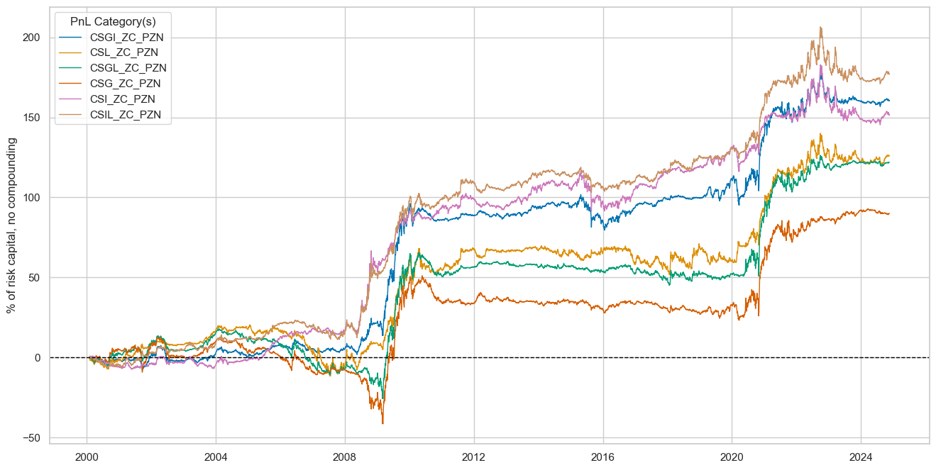
dix = dict_eqdi

sigx = dix["rivs"]
naive_pnl = dix["pnls"]
pnls = [sig + "_PZN" for sig in sigx]

naive_pnl.plot_pnls(
    pnl_cats=pnls,
    pnl_cids=["ALL"],
    start="2000-01-01",
    title=None,
    xcat_labels=None,
    figsize=(16, 8),
)

dix = dict_eqdi

sigx = [dix["sig"]] + dix["rivs"]
naive_pnl = dix["pnls"]
pnls = [sig + type for sig in sigx for type in ["_PZN", "_BIN"]]

df_eval = naive_pnl.evaluate_pnls(
    pnl_cats=pnls,
    pnl_cids=["ALL"],
    start="2000-01-01",
)
display(df_eval.transpose())

	Return %	St. Dev. %	Sharpe Ratio	Sortino Ratio	Max 21-Day Draw %	Max 6-Month Draw %	Peak to Trough Draw %	Top 5% Monthly PnL Share	USD_EQXR_NSA correl	Traded Months
xcat
CSGIL_ZC_PZN	6.94022	10.0	0.694022	1.056501	-16.166429	-16.223607	-22.790915	0.928508	0.017189	298
CSGI_ZC_PZN	6.477148	10.0	0.647715	0.969935	-15.512794	-16.084488	-22.115923	0.955529	0.10583	298
CSL_ZC_PZN	5.084576	10.0	0.508458	0.763275	-16.256005	-15.15405	-32.059263	1.02996	-0.166519	298
CSGL_ZC_PZN	4.921142	10.0	0.492114	0.755367	-16.141134	-19.189023	-43.66662	1.277214	0.091609	298
CSG_ZC_PZN	3.633014	10.0	0.363301	0.552031	-14.719867	-27.121756	-54.156334	1.680659	0.252896	298
CSI_ZC_PZN	6.113695	10.0	0.61137	0.88192	-19.795761	-24.688366	-37.621333	0.89019	-0.099871	298
CSIL_ZC_PZN	7.147002	10.0	0.7147	1.058185	-19.836399	-23.354137	-35.725208	0.830926	-0.156898	298
CSGIL_ZC_BIN	5.023701	10.0	0.50237	0.731789	-12.466828	-15.689518	-32.402217	0.949469	-0.037476	298
CSGI_ZC_BIN	5.67273	10.0	0.567273	0.81104	-15.337639	-18.773117	-27.927563	0.822128	0.049908	298
CSL_ZC_BIN	3.122454	10.0	0.312245	0.470511	-12.794928	-18.429408	-46.73745	1.494443	-0.232358	298
CSGL_ZC_BIN	-0.231495	10.0	-0.023149	-0.033609	-12.35682	-20.250482	-64.493563	-19.652593	-0.00372	298
CSG_ZC_BIN	1.415129	10.0	0.141513	0.201447	-22.879402	-24.320621	-50.514564	3.033367	0.20364	298
CSI_ZC_BIN	6.584364	10.0	0.658436	0.930802	-21.426654	-16.073625	-31.616623	0.71571	-0.009845	298
CSIL_ZC_BIN	6.001176	10.0	0.600118	0.868822	-13.391313	-19.065276	-34.175308	0.821154	-0.127269	298

dix = dict_eqdi
sig = dix["sig"]
naive_pnl = dix["pnls"]

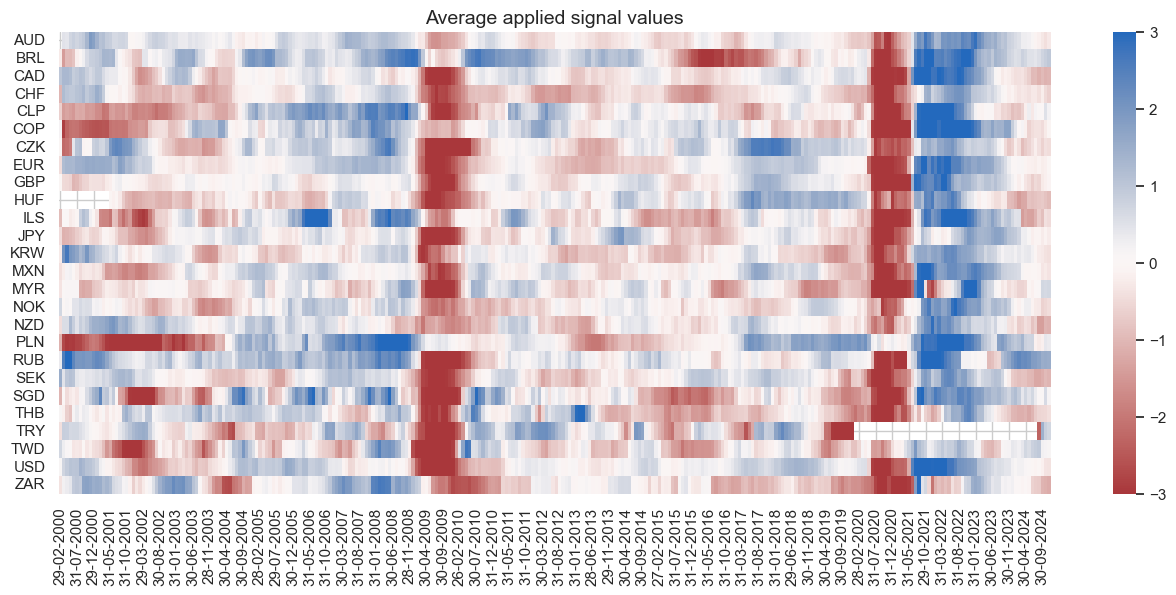
naive_pnl.signal_heatmap(
    pnl_name=sig + "_PZN", freq="q", start="2000-01-01", figsize=(16, 5)
)

Directional FX strategy

Specs and panel test

sigs = cs_rel
ms = "CSGILvBM_ZC"  # main signal
oths = list(set(sigs) - set([ms]))  # other signals

targ = "FXXR_VT10"
cidx = msm.common_cids(dfx, sigs + [targ])
# cidx = list(set(cids_dm) & set(cidx))   # for DM alone

dict_fxdi = {
    "sig": ms,
    "rivs": oths,
    "targ": targ,
    "cidx": cidx,
    "black": None,
    "srr": None,
    "pnls": None,
}

dix = dict_fxdi

sig = dix["sig"]
targ = dix["targ"]
cidx = dix["cidx"]
blax = dix["black"]

crx = msp.CategoryRelations(
    dfx,
    xcats=[sig, targ],
    cids=cidx,
    freq="Q",  # quarterly frequency allows for policy inertia
    lag=1,
    xcat_aggs=["last", "sum"],
    start="2000-01-01",
    blacklist=blax,
    xcat_trims=[1000, 40],
)
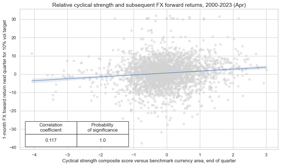
crx.reg_scatter(
    labels=False,
    coef_box="lower left",
    xlab="Cyclical strength composite score versus benchmark currency area, end of quarter",
    ylab="1-month FX foward return next quarter for 10% vol target",
    title="Relative cyclical strength and subsequent FX forward returns, 2000-2023 (Apr)",
    size=(10, 6),
    prob_est="map",
)

Accuracy and correlation check

dix = dict_fxdi

sig = dix["sig"]
rivs = dix["rivs"]
targ = dix["targ"]
cidx = dix["cidx"]
blax = dix["black"]

srr = mss.SignalReturnRelations(
    dfx,
    cids=cidx,
    sigs=[sig] + rivs,
    rets=targ,
    freqs="M",
    start="2000-01-01",
    blacklist=blax,
)

dix["srr"] = srr

dix = dict_fxdi
srrx = dix["srr"]
display(srrx.summary_table().astype("float").round(3))

	accuracy	bal_accuracy	pos_sigr	pos_retr	pos_prec	neg_prec	pearson	pearson_pval	kendall	kendall_pval	auc
M: CSGILvBM_ZC/last => FXXR_VT10	0.521	0.525	0.456	0.545	0.572	0.478	0.073	0.000	0.049	0.000	0.525
Mean years	0.520	0.517	0.454	0.545	0.561	0.473	0.062	0.319	0.036	0.287	0.515
Positive ratio	0.680	0.720	0.440	0.680	0.760	0.320	0.800	0.680	0.800	0.680	0.720
Mean cids	0.521	0.520	0.459	0.546	0.569	0.472	0.069	0.306	0.042	0.355	0.520
Positive ratio	0.741	0.741	0.296	0.852	0.852	0.333	0.815	0.667	0.778	0.556	0.741

dix = dict_fxdi
srrx = dix["srr"]
display(srrx.signals_table().sort_index().astype("float").round(3))

				accuracy	bal_accuracy	pos_sigr	pos_retr	pos_prec	neg_prec	pearson	pearson_pval	kendall	kendall_pval	auc
Return	Signal	Frequency	Aggregation
FXXR_VT10	CSGILvBM_ZC	M	last	0.521	0.525	0.456	0.545	0.572	0.478	0.073	0.000	0.049	0.000	0.525
	CSGIvBM_ZC	M	last	0.510	0.512	0.469	0.544	0.557	0.468	0.051	0.000	0.033	0.000	0.512
	CSGLvBM_ZC	M	last	0.520	0.522	0.478	0.545	0.568	0.476	0.059	0.000	0.043	0.000	0.522
	CSGvBM_ZC	M	last	0.512	0.513	0.480	0.539	0.552	0.474	0.023	0.048	0.016	0.037	0.513
	CSILvBM_ZC	M	last	0.528	0.531	0.469	0.544	0.577	0.485	0.082	0.000	0.056	0.000	0.531
	CSIvBM_ZC	M	last	0.516	0.518	0.470	0.541	0.561	0.476	0.054	0.000	0.036	0.000	0.519
	CSLvBM_ZC	M	last	0.526	0.528	0.472	0.543	0.573	0.484	0.074	0.000	0.056	0.000	0.528

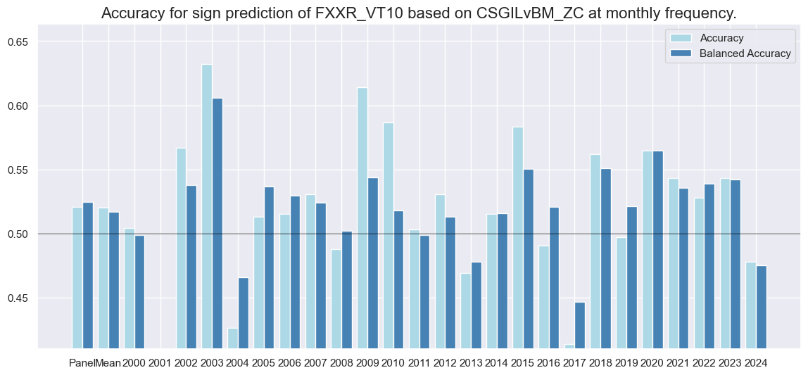
dix = dict_fxdi
srrx = dix["srr"]
srrx.accuracy_bars(
    type="years",
    # title="",
    size=(14, 6),
)

Naive PnL

dix = dict_fxdi

sigx = [dix["sig"]] + dix["rivs"]
targ = dix["targ"]
cidx = dix["cidx"]
blax = dix["black"]

naive_pnl = msn.NaivePnL(
    dfx,
    ret=targ,
    sigs=sigx,
    cids=cidx,
    start="2000-01-01",
    blacklist=blax,
    bms=["USD_EQXR_NSA"],
)

for sig in sigx:
    naive_pnl.make_pnl(
        sig,
        sig_neg=False,
        sig_op="zn_score_pan",
        thresh=3,
        rebal_freq="monthly",
        vol_scale=10,
        rebal_slip=1,
        pnl_name=sig + "_PZN",
    )

for sig in sigx:
    naive_pnl.make_pnl(
        sig,
        sig_neg=False,
        sig_op="binary",
        thresh=3,
        rebal_freq="monthly",
        vol_scale=10,
        rebal_slip=1,
        pnl_name=sig + "_BIN",
    )

naive_pnl.make_long_pnl(vol_scale=10, label="Long only")
dix["pnls"] = naive_pnl

dix = dict_fxdi

sigx = dix["sig"]
naive_pnl = dix["pnls"]
pnls = [sigx + x for x in ["_PZN", "_BIN"]] + ["Long only"]

naive_pnl.plot_pnls(
    pnl_cats=pnls,
    pnl_cids=["ALL"],
    start="2000-01-01",
    title=None,
    xcat_labels=None,
    figsize=(16, 8),
)

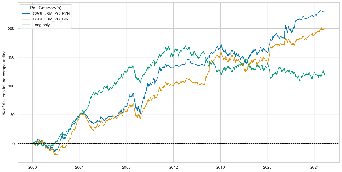
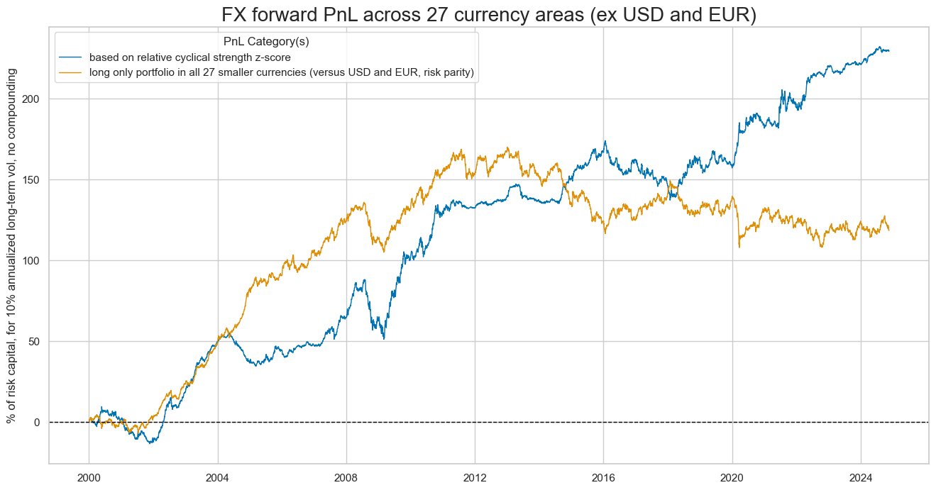
dix = dict_fxdi

sigx = dix["sig"]
naive_pnl = dix["pnls"]
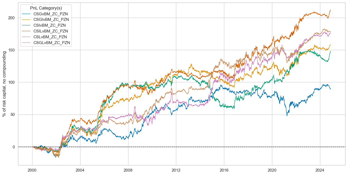
pnls = [sigx + "_PZN"] + ["Long only"]

dict_labels={"CSGILvBM_ZC_PZN":"based on relative cyclical strength z-score",
"Long only": "long only portfolio in all 27 smaller currencies (versus USD and EUR, risk parity)"}

naive_pnl.plot_pnls(
    pnl_cats=pnls,
    pnl_cids=["ALL"],
    start="2000-01-01",
    title="FX forward PnL across 27 currency areas (ex USD and EUR)",
    xcat_labels=dict_labels,
    ylab="% of risk capital, for 10% annualized long-term vol, no compounding",
    figsize=(16, 8),
)

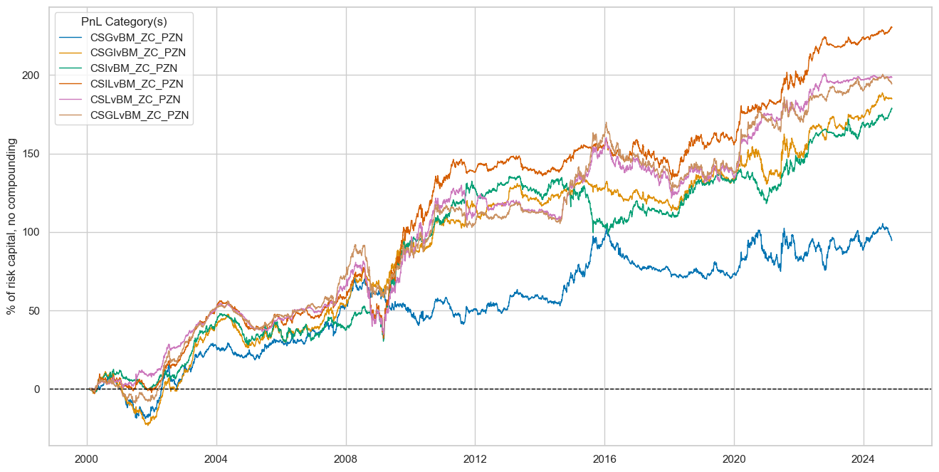
dix = dict_fxdi

sigx = dix["rivs"]
naive_pnl = dix["pnls"]
pnls = [sig + "_PZN" for sig in sigx]

naive_pnl.plot_pnls(
    pnl_cats=pnls,
    pnl_cids=["ALL"],
    start="2000-01-01",
    title=None,
    xcat_labels=None,
    figsize=(16, 8),
)

dix = dict_fxdi

sigx = [dix["sig"]] + dix["rivs"]
naive_pnl = dix["pnls"]
pnls = [sig + type for sig in sigx for type in ["_PZN", "_BIN"]]

df_eval = naive_pnl.evaluate_pnls(
    pnl_cats=pnls,
    pnl_cids=["ALL"],
    start="2000-01-01",
)
display(df_eval.transpose())

	Return %	St. Dev. %	Sharpe Ratio	Sortino Ratio	Max 21-Day Draw %	Max 6-Month Draw %	Peak to Trough Draw %	Top 5% Monthly PnL Share	USD_EQXR_NSA correl	Traded Months
xcat
CSGILvBM_ZC_PZN	9.261088	10.0	0.926109	1.382363	-15.673803	-29.756144	-37.090776	0.570461	0.066619	298
CSGvBM_ZC_PZN	3.827413	10.0	0.382741	0.557852	-14.212981	-22.414324	-32.459905	1.31609	-0.043541	298
CSGIvBM_ZC_PZN	7.456637	10.0	0.745664	1.115362	-10.217006	-22.244731	-34.453754	0.738076	0.058735	298
CSIvBM_ZC_PZN	7.197503	10.0	0.71975	1.069246	-14.530983	-25.393154	-37.485675	0.716886	0.121809	298
CSILvBM_ZC_PZN	9.288838	10.0	0.928884	1.380198	-17.483943	-31.51101	-45.263751	0.587457	0.105013	298
CSLvBM_ZC_PZN	8.007575	10.0	0.800757	1.167653	-21.942334	-39.163553	-46.777365	0.67673	0.060382	298
CSGLvBM_ZC_PZN	7.844372	10.0	0.784437	1.163382	-16.817638	-30.414612	-43.802041	0.691028	0.015146	298
CSGILvBM_ZC_BIN	8.00653	10.0	0.800653	1.200041	-11.132284	-22.971975	-38.928926	0.66176	0.018296	298
CSGvBM_ZC_BIN	4.778669	10.0	0.477867	0.683746	-15.351668	-18.663776	-25.745332	1.076229	-0.054738	298
CSGIvBM_ZC_BIN	3.096388	10.0	0.309639	0.450092	-11.777379	-23.954522	-39.199084	1.472184	0.059299	298
CSIvBM_ZC_BIN	4.106984	10.0	0.410698	0.597581	-10.785082	-20.777816	-34.399829	1.100338	0.085428	298
CSILvBM_ZC_BIN	8.16824	10.0	0.816824	1.215106	-16.001452	-27.950346	-34.228853	0.63867	0.050056	298
CSLvBM_ZC_BIN	6.899793	10.0	0.689979	0.99368	-16.002236	-32.63338	-40.039205	0.790295	0.002617	298
CSGLvBM_ZC_BIN	6.053429	10.0	0.605343	0.865733	-16.844083	-26.114256	-49.717024	0.846229	0.002384	298

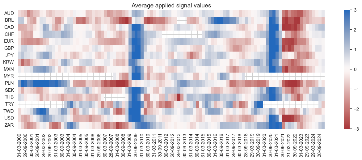
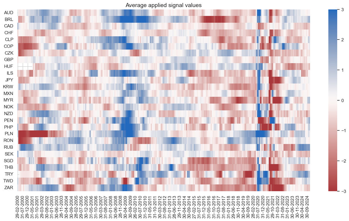
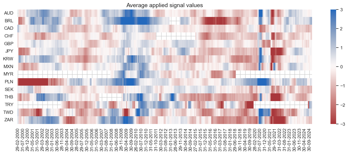
dix = dict_fxdi
sig = dix["sig"]
naive_pnl = dix["pnls"]

naive_pnl.signal_heatmap(
    pnl_name=sig + "_PZN", freq="m", start="2000-01-01", figsize=(16, 8)
)

Directional IRS strategy

Specs and panel test

sigs = cs_dir
ms = "CSGIL_ZC"  # main signal
oths = list(set(sigs) - set([ms]))  # other signals

targ = "DU05YXR_VT10"  # "DU02YXR_VT10"
cidx = msm.common_cids(dfx, sigs + [targ])
# cidx = list(set(cids_dm) & set(cidx))   # for DM alone

dict_dudi = {
    "sig": ms,
    "rivs": oths,
    "targ": targ,
    "cidx": cidx,
    "black": dublack,
    "srr": None,
    "pnls": None,
}

dix = dict_dudi
cidx = dix["cidx"]
print(len(cidx))
", ".join(cidx)

26

'AUD, BRL, CAD, CHF, CLP, COP, CZK, EUR, GBP, HUF, ILS, JPY, KRW, MXN, MYR, NOK, NZD, PLN, RUB, SEK, SGD, THB, TRY, TWD, USD, ZAR'

dix = dict_dudi

sig = dix["sig"]
targ = dix["targ"]
cidx = dix["cidx"]
blax = dix["black"]

crx = msp.CategoryRelations(
    dfx,
    xcats=[sig, targ],
    cids=cidx,
    freq="Q",
    lag=1,
    xcat_aggs=["last", "sum"],
    start="2000-01-01",
    blacklist=blax,
    xcat_trims=[None, None],
)
crx.reg_scatter(
    labels=False,
    coef_box="lower left",
    xlab="Cyclical strength composite score, end of quarter",
    ylab="5-year IRS return next quarter for 10% vol target",
    title="Cyclical strength and subsequent 5-year IRS returns, 2000-2023 (Apr)",
    size=(10, 6),
    prob_est="map",
)

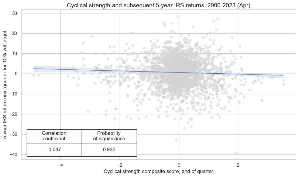
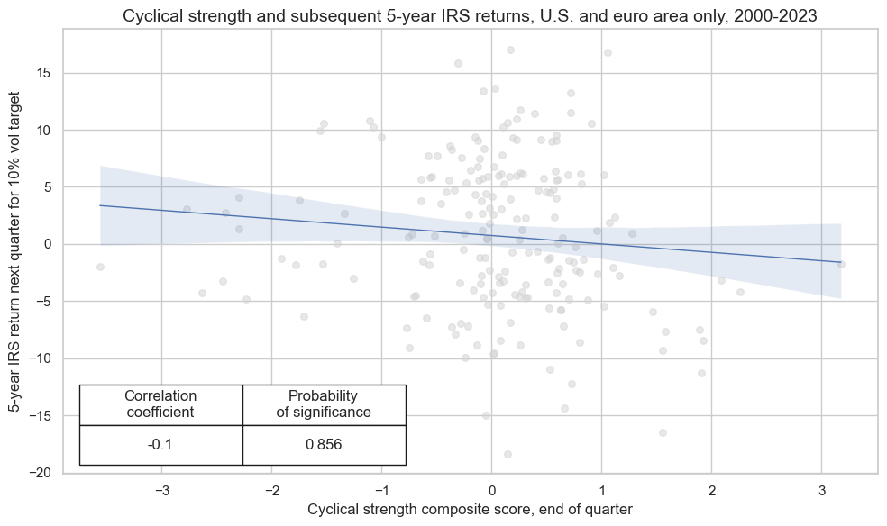
dix = dict_dudi

sig = dix["sig"]
targ = dix["targ"]
cidx = ["EUR", "USD"]
blax = dix["black"]

crx = msp.CategoryRelations(
    dfx,
    xcats=[sig, targ],
    cids=cidx,
    freq="Q",
    lag=1,
    xcat_aggs=["last", "sum"],
    start="2000-01-01",
    blacklist=blax,
    xcat_trims=[None, None],
)
crx.reg_scatter(
    labels=False,
    coef_box="lower left",
    xlab="Cyclical strength composite score, end of quarter",
    ylab="5-year IRS return next quarter for 10% vol target",
    title="Cyclical strength and subsequent 5-year IRS returns, U.S. and euro area only, 2000-2023",
    size=(10, 6),
    prob_est="map",
)

Accuracy and correlation check

dix = dict_dudi

sig = dix["sig"]
rivs = dix["rivs"]
targ = dix["targ"]
cidx = dix["cidx"]
blax = dix["black"]

srr = mss.SignalReturnRelations(
    dfx,
    cids=cidx,
    sigs=[sig] + rivs,
    sig_neg=[True] + [True] * len(rivs),
    rets=targ,
    freqs="M",
    start="2000-01-01",
    blacklist=blax,
)

dix["srr"] = srr

dix = dict_dudi
srrx = dix["srr"]
display(srrx.summary_table().astype("float").round(3))

	accuracy	bal_accuracy	pos_sigr	pos_retr	pos_prec	neg_prec	pearson	pearson_pval	kendall	kendall_pval	auc
M: CSGIL_ZC_NEG/last => DU05YXR_VT10	0.527	0.527	0.502	0.546	0.573	0.482	0.046	0.000	0.034	0.000	0.527
Mean years	0.520	0.514	0.496	0.556	0.571	0.457	0.017	0.385	0.017	0.391	0.513
Positive ratio	0.640	0.680	0.480	0.800	0.760	0.360	0.560	0.400	0.560	0.440	0.680
Mean cids	0.527	0.527	0.498	0.544	0.572	0.482	0.045	0.457	0.032	0.485	0.527
Positive ratio	0.885	0.923	0.462	0.962	1.000	0.308	0.808	0.538	0.846	0.500	0.923

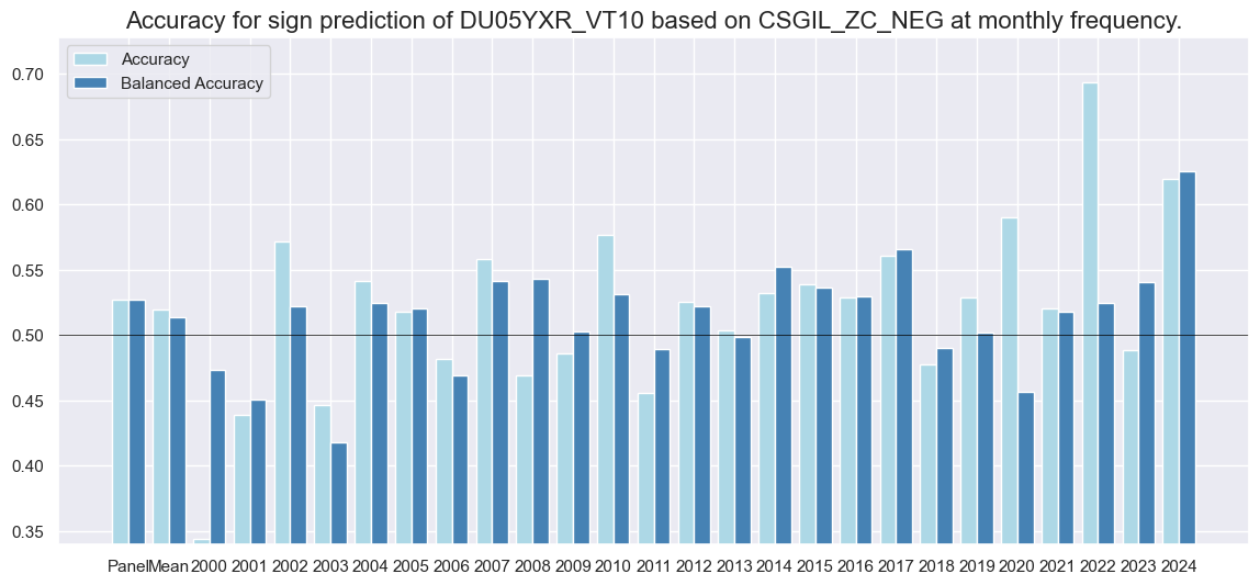
Labor market dynamics are good predictors, labor market status is not, supporting the hypothesis that fixed-income markets are only inattentive to recent dynamics but not to the broad state of the economy.

dix = dict_dudi
srrx = dix["srr"]
display(srrx.signals_table().sort_index().astype("float").round(3))

				accuracy	bal_accuracy	pos_sigr	pos_retr	pos_prec	neg_prec	pearson	pearson_pval	kendall	kendall_pval	auc
Return	Signal	Frequency	Aggregation
DU05YXR_VT10	CSGIL_ZC_NEG	M	last	0.527	0.527	0.502	0.546	0.573	0.482	0.046	0.000	0.034	0.000	0.527
	CSGI_ZC_NEG	M	last	0.529	0.524	0.562	0.546	0.567	0.482	0.049	0.000	0.033	0.000	0.524
	CSGL_ZC_NEG	M	last	0.513	0.516	0.462	0.546	0.563	0.469	0.035	0.004	0.033	0.000	0.516
	CSG_ZC_NEG	M	last	0.516	0.512	0.549	0.546	0.556	0.467	0.033	0.007	0.029	0.000	0.512
	CSIL_ZC_NEG	M	last	0.520	0.521	0.484	0.546	0.568	0.475	0.040	0.001	0.030	0.000	0.522
	CSI_ZC_NEG	M	last	0.525	0.522	0.536	0.545	0.565	0.479	0.035	0.004	0.027	0.001	0.522
	CSL_ZC_NEG	M	last	0.502	0.514	0.377	0.545	0.563	0.465	0.026	0.040	0.026	0.002	0.513

dix = dict_dudi
srrx = dix["srr"]
srrx.accuracy_bars(
    type="years",
    # title="Accuracy of monthly predictions of FX forward returns for 26 EM and DM currencies",
    size=(14, 6),
)

Naive PnL

dix = dict_dudi

sigx = [dix["sig"]] + dix["rivs"]
targ = dix["targ"]
cidx = dix["cidx"]
blax = dix["black"]

naive_pnl = msn.NaivePnL(
    dfx,
    ret=targ,
    sigs=sigx,
    cids=cidx,
    start="2000-01-01",
    blacklist=blax,
    bms=["USD_EQXR_NSA", "USD_DU05YXR_VT10"],
)

for sig in sigx:
    naive_pnl.make_pnl(
        sig,
        sig_neg=True,
        sig_op="zn_score_pan",
        thresh=3,
        rebal_freq="monthly",
        vol_scale=10,
        rebal_slip=1,
        pnl_name=sig + "_PZN",
    )

for sig in sigx:
    naive_pnl.make_pnl(
        sig,
        sig_neg=True,
        sig_op="binary",
        thresh=3,
        rebal_freq="monthly",
        vol_scale=10,
        rebal_slip=1,
        pnl_name=sig + "_BIN",
    )

naive_pnl.make_long_pnl(vol_scale=10, label="Long only")
dix["pnls"] = naive_pnl

dix = dict_dudi

sigx = dix["sig"]
naive_pnl = dix["pnls"]
pnls = [sigx + x for x in ["_PZN", "_BIN"]] + ["Long only"]

naive_pnl.plot_pnls(
    pnl_cats=pnls,
    pnl_cids=["ALL"],
    start="2000-01-01",
    title=None,
    xcat_labels=None,
    figsize=(16, 8),
)

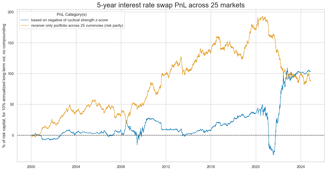
dix = dict_dudi

sigx = dix["sig"]
naive_pnl = dix["pnls"]
pnls = [sigx + "_PZN"] + ["Long only"]

dict_labels={"CSGIL_ZC_PZN":"based on negative of cyclical strength z-score",
"Long only": "receiver only portfolio across 25 currencies (risk parity)"}

naive_pnl.plot_pnls(
    pnl_cats=pnls,
    pnl_cids=["ALL"],
    start="2000-01-01",
    title="5-year interest rate swap PnL across 25 markets",
    xcat_labels=dict_labels,
    ylab="% of risk capital, for 10% annualized long-term vol, no compounding",
    figsize=(16, 8),
)

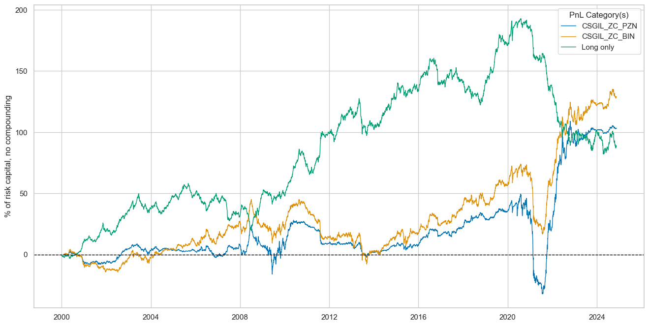
dix = dict_dudi

sigx = dix["rivs"]
naive_pnl = dix["pnls"]
pnls = [sig + "_PZN" for sig in sigx]

naive_pnl.plot_pnls(
    pnl_cats=pnls,
    pnl_cids=["ALL"],
    start="2000-01-01",
    title=None,
    xcat_labels=None,
    figsize=(16, 8),
)

dix = dict_dudi

sigx = [dix["sig"]] + dix["rivs"]
naive_pnl = dix["pnls"]
pnls = [sig + type for sig in sigx for type in ["_PZN", "_BIN"]]

df_eval = naive_pnl.evaluate_pnls(
    pnl_cats=pnls,
    pnl_cids=["ALL"],
    start="2000-01-01",
)
display(df_eval.transpose())

	Return %	St. Dev. %	Sharpe Ratio	Sortino Ratio	Max 21-Day Draw %	Max 6-Month Draw %	Peak to Trough Draw %	Top 5% Monthly PnL Share	USD_EQXR_NSA correl	USD_DU05YXR_VT10 correl	Traded Months
xcat
CSGIL_ZC_PZN	4.16784	10.0	0.416784	0.575774	-45.793736	-67.90159	-81.675222	1.833909	-0.047435	-0.005533	298
CSGI_ZC_PZN	4.923035	10.0	0.492303	0.688027	-42.362385	-63.929288	-78.310767	1.560824	-0.069614	0.082674	298
CSL_ZC_PZN	1.874711	10.0	0.187471	0.256665	-42.063428	-60.010895	-110.758683	3.355906	0.02001	-0.203839	298
CSGL_ZC_PZN	3.624902	10.0	0.36249	0.492273	-52.584546	-79.874424	-96.209772	1.924651	-0.023304	-0.02364	298
CSG_ZC_PZN	4.660084	10.0	0.466008	0.644726	-49.787496	-77.317165	-94.870154	1.558637	-0.044899	0.102364	298
CSI_ZC_PZN	3.40874	10.0	0.340874	0.481672	-18.305893	-56.67491	-96.044596	2.168579	-0.072866	0.021042	298
CSIL_ZC_PZN	3.285492	10.0	0.328549	0.458652	-30.479786	-48.210489	-72.383527	2.294462	-0.041852	-0.074072	298
CSGIL_ZC_BIN	5.209368	10.0	0.520937	0.72154	-33.637271	-47.903753	-57.261791	1.195209	-0.036136	-0.002175	298
CSGI_ZC_BIN	5.29339	10.0	0.529339	0.730874	-32.710023	-48.204066	-55.429584	1.182556	-0.063886	0.12569	298
CSL_ZC_BIN	0.136479	10.0	0.013648	0.018785	-33.96345	-44.599902	-111.873536	41.690982	0.034115	-0.27327	298
CSGL_ZC_BIN	3.087066	10.0	0.308707	0.433864	-34.966363	-51.422782	-77.502358	2.06416	-0.034532	-0.130907	298
CSG_ZC_BIN	4.083461	10.0	0.408346	0.579857	-33.989599	-49.986319	-66.301527	1.572367	-0.058698	0.085706	298
CSI_ZC_BIN	3.390662	10.0	0.339066	0.474978	-20.217069	-46.042963	-93.982369	1.87593	-0.059971	0.091732	298
CSIL_ZC_BIN	1.96615	10.0	0.196615	0.269282	-25.119427	-44.794831	-84.641031	2.8204	-0.005302	-0.037401	298

dix = dict_dudi
sig = dix["sig"]
naive_pnl = dix["pnls"]

naive_pnl.signal_heatmap(
    pnl_name=sig + "_PZN", freq="m", start="2000-01-01", figsize=(16, 8)
)

FX versus equity strategy (directional features)

Specs and panel test

sigs = cs_dir
ms = "CSGIL_ZC"  # main signal
oths = list(set(sigs) - set([ms]))  # other signals

targ = "FXvEQXR"
cidx = msm.common_cids(dfx, sigs + [targ])
cidx = list(set(cidx_fxeq) & set(cidx))
dict_fxeq = {
    "sig": ms,
    "rivs": oths,
    "targ": targ,
    "cidx": cidx,
    "black": fxblack,
    "srr": None,
    "pnls": None,
}

dix = dict_fxeq
cidx = dix["cidx"]
cidx.sort()
print(len(cidx))
", ".join(cidx)

17

'AUD, BRL, CAD, CHF, EUR, GBP, JPY, KRW, MXN, MYR, PLN, SEK, SGD, THB, TRY, TWD, ZAR'

dix = dict_fxeq

sig = dix["sig"]
targ = dix["targ"]
cidx = dix["cidx"]
blax = dix["black"]

crx = msp.CategoryRelations(
    dfx,
    xcats=[sig, targ],
    cids=cidx,
    freq="Q",  # quarterly frequency allows for policy inertia
    lag=1,
    xcat_aggs=["last", "sum"],
    start="2000-01-01",
    blacklist=blax,
    xcat_trims=[None, None],
)
crx.reg_scatter(
    labels=False,
    coef_box="lower left",
    xlab="Cyclical strength composite score, end of quarter",
    ylab="FX forward versus equity future return next quarter (both 10% vol target)",
    title="Cyclical strength and subsequent FX versus equity returns, 2000-2023 (Apr)",
    size=(10, 6),
    prob_est="map",
)

Accuracy and correlation check

dix = dict_fxeq

sig = dix["sig"]
rivs = dix["rivs"]
targ = dix["targ"]
cidx = dix["cidx"]
blax = dix["black"]

srr = mss.SignalReturnRelations(
    dfx,
    cids=cidx,
    sigs=[sig] + rivs,
    rets=targ,
    freqs="M",
    start="2000-01-01",
    blacklist=blax,
)

dix["srr"] = srr

dix = dict_fxeq
srrx = dix["srr"]
display(srrx.summary_table().astype("float").round(3))

	accuracy	bal_accuracy	pos_sigr	pos_retr	pos_prec	neg_prec	pearson	pearson_pval	kendall	kendall_pval	auc
M: CSGIL_ZC/last => FXvEQXR	0.518	0.517	0.486	0.460	0.477	0.557	0.047	0.003	0.029	0.006	0.517
Mean years	0.517	0.508	0.491	0.461	0.466	0.551	0.046	0.396	0.016	0.430	0.506
Positive ratio	0.680	0.480	0.400	0.280	0.280	0.720	0.680	0.360	0.480	0.320	0.480
Mean cids	0.519	0.513	0.489	0.462	0.474	0.551	0.042	0.494	0.025	0.461	0.512
Positive ratio	0.812	0.688	0.500	0.125	0.250	0.750	0.688	0.625	0.750	0.438	0.688

dix = dict_fxeq
srrx = dix["srr"]
display(srrx.signals_table().sort_index().astype("float").round(3))

				accuracy	bal_accuracy	pos_sigr	pos_retr	pos_prec	neg_prec	pearson	pearson_pval	kendall	kendall_pval	auc
Return	Signal	Frequency	Aggregation
FXvEQXR	CSGIL_ZC	M	last	0.518	0.517	0.486	0.459	0.477	0.557	0.047	0.003	0.029	0.006	0.517
	CSGI_ZC	M	last	0.519	0.514	0.442	0.460	0.476	0.553	0.035	0.026	0.023	0.031	0.514
	CSGL_ZC	M	last	0.497	0.500	0.546	0.459	0.460	0.541	0.027	0.084	0.014	0.177	0.500
	CSG_ZC	M	last	0.501	0.497	0.456	0.460	0.456	0.538	0.006	0.680	-0.003	0.798	0.497
	CSIL_ZC	M	last	0.516	0.516	0.497	0.459	0.476	0.557	0.067	0.000	0.040	0.000	0.516
	CSI_ZC	M	last	0.523	0.519	0.447	0.460	0.481	0.557	0.051	0.001	0.033	0.001	0.519
	CSL_ZC	M	last	0.504	0.513	0.601	0.459	0.469	0.556	0.049	0.002	0.033	0.002	0.512

dix = dict_fxeq
srrx = dix["srr"]
srrx.accuracy_bars(
    type="years",
    title="Accuracy of monthly predictions of FX forward returns for 26 EM and DM currencies",
    size=(14, 6),
)

Naive PnL

dix = dict_fxeq

sigx = [dix["sig"]] + dix["rivs"]
targ = dix["targ"]
cidx = dix["cidx"]
blax = dix["black"]

naive_pnl = msn.NaivePnL(
    dfx,
    ret=targ,
    sigs=sigx,
    cids=cidx,
    start="2000-01-01",
    blacklist=blax,
    bms=["USD_EQXR_NSA"],
)

for sig in sigx:
    naive_pnl.make_pnl(
        sig,
        sig_neg=False,
        sig_op="zn_score_pan",
        thresh=3,
        rebal_freq="monthly",
        vol_scale=10,
        rebal_slip=1,
        pnl_name=sig + "_PZN",
    )

for sig in sigx:
    naive_pnl.make_pnl(
        sig,
        sig_neg=False,
        sig_op="binary",
        thresh=3,
        rebal_freq="monthly",
        vol_scale=10,
        rebal_slip=1,
        pnl_name=sig + "_BIN",
    )

naive_pnl.make_long_pnl(vol_scale=10, label="Long only")
dix["pnls"] = naive_pnl

dix = dict_fxeq

sigx = dix["sig"]
naive_pnl = dix["pnls"]
pnls = [sigx + x for x in ["_PZN", "_BIN"]] + ["Long only"]

naive_pnl.plot_pnls(
    pnl_cats=pnls,
    pnl_cids=["ALL"],
    start="2000-01-01",
    title=None,
    xcat_labels=None,
    figsize=(16, 8),
)

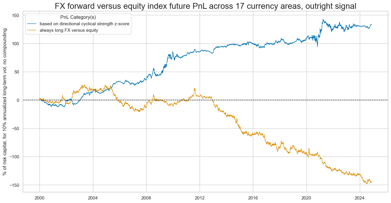
dix = dict_fxeq

sigx = dix["sig"]
naive_pnl = dix["pnls"]
pnls = [sigx + "_PZN"] + ["Long only"]

dict_labels={"CSGIL_ZC_PZN":"based on directional cyclical strength z-score",
"Long only": "always long FX versus equity"}

naive_pnl.plot_pnls(
    pnl_cats=pnls,
    pnl_cids=["ALL"],
    start="2000-01-01",
    title="FX forward versus equity index future PnL across 17 currency areas, outright signal",
    xcat_labels=dict_labels,
    ylab="% of risk capital, for 10% annualized long-term vol, no compounding",
    figsize=(16, 8),
)

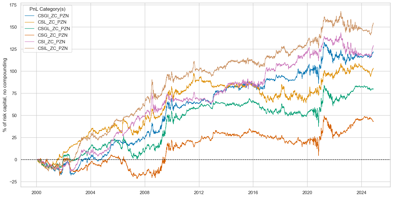
dix = dict_fxeq

sigx = dix["rivs"]
naive_pnl = dix["pnls"]
pnls = [sig + "_PZN" for sig in sigx]

naive_pnl.plot_pnls(
    pnl_cats=pnls,
    pnl_cids=["ALL"],
    start="2000-01-01",
    title=None,
    xcat_labels=None,
    figsize=(16, 8),
)

dix = dict_fxeq

sigx = [dix["sig"]] + dix["rivs"]
naive_pnl = dix["pnls"]
pnls = [sig + type for sig in sigx for type in ["_PZN", "_BIN"]]

df_eval = naive_pnl.evaluate_pnls(
    pnl_cats=pnls,
    pnl_cids=["ALL"],
    start="2000-01-01",
)
display(df_eval.transpose())

	Return %	St. Dev. %	Sharpe Ratio	Sortino Ratio	Max 21-Day Draw %	Max 6-Month Draw %	Peak to Trough Draw %	Top 5% Monthly PnL Share	USD_EQXR_NSA correl	Traded Months
xcat
CSGIL_ZC_PZN	5.404663	10.0	0.540466	0.793665	-15.437734	-18.211074	-22.363847	0.991188	0.033378	298
CSGI_ZC_PZN	4.913452	10.0	0.491345	0.707903	-15.231804	-20.778578	-25.644142	1.084504	0.10942	298
CSL_ZC_PZN	4.160296	10.0	0.41603	0.613842	-11.552108	-16.627945	-33.648778	1.030258	-0.135208	298
CSGL_ZC_PZN	3.235519	10.0	0.323552	0.478286	-16.589878	-19.892795	-31.831864	1.624277	0.033973	298
CSG_ZC_PZN	1.754645	10.0	0.175465	0.256299	-16.158822	-23.622871	-30.677551	2.827893	0.150313	298
CSI_ZC_PZN	5.181652	10.0	0.518165	0.730243	-18.322582	-19.412635	-28.085692	0.822389	0.026168	298
CSIL_ZC_PZN	6.211037	10.0	0.621104	0.90086	-17.658517	-19.72873	-26.851595	0.753829	-0.050241	298
CSGIL_ZC_BIN	5.029814	10.0	0.502981	0.72627	-12.058163	-18.563666	-22.077322	0.930152	0.00776	298
CSGI_ZC_BIN	4.445168	10.0	0.444517	0.632069	-14.878733	-18.899299	-26.300824	1.011533	0.070574	298
CSL_ZC_BIN	1.955155	10.0	0.195515	0.283652	-12.969751	-19.178251	-54.400372	2.08257	-0.173999	298
CSGL_ZC_BIN	0.476751	10.0	0.047675	0.068455	-12.738207	-27.516349	-63.809396	8.66207	-0.004902	298
CSG_ZC_BIN	0.731409	10.0	0.073141	0.103483	-17.46463	-18.319009	-39.833391	5.953649	0.12874	298
CSI_ZC_BIN	5.706193	10.0	0.570619	0.797082	-13.322301	-13.988839	-26.350624	0.730147	0.073024	298
CSIL_ZC_BIN	4.963421	10.0	0.496342	0.715104	-13.838683	-16.530162	-36.938316	0.903859	-0.023113	298

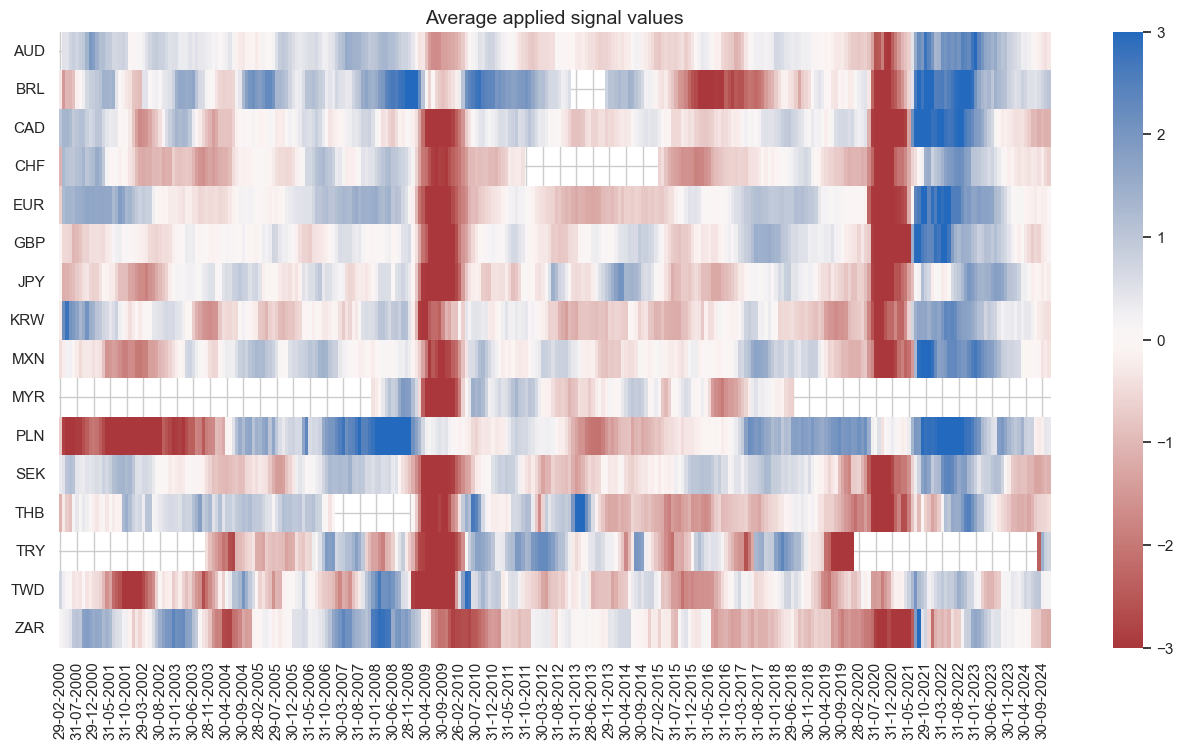
dix = dict_fxeq
sig = dix["sig"]
naive_pnl = dix["pnls"]

naive_pnl.signal_heatmap(
    pnl_name=sig + "_PZN", freq="m", start="2000-01-01", figsize=(16, 8)
)

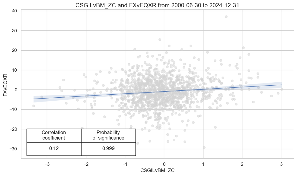
FX versus equity strategy (relative features)

Specs and panel test

sigs = cs_rel
ms = "CSGILvBM_ZC"  # main signal
oths = list(set(sigs) - set([ms]))  # other signals

targ = "FXvEQXR"
cidx = msm.common_cids(dfx, sigs + [targ])
cidx = list(set(cidx_fxeq) & set(cidx))
dict_fxeq_rf = {
    "sig": ms,
    "rivs": oths,
    "targ": targ,
    "cidx": cidx,
    "black": fxblack,
    "srr": None,
    "pnls": None,
}

dix = dict_fxeq_rf

sig = dix["sig"]
targ = dix["targ"]
cidx = dix["cidx"]
blax = dix["black"]

crx = msp.CategoryRelations(
    dfx,
    xcats=[sig, targ],
    cids=cidx,
    freq="Q",  # quarterly frequency allows for policy inertia
    lag=1,
    xcat_aggs=["last", "sum"],
    start="2000-01-01",
    blacklist=blax,
    xcat_trims=[None, None],
)
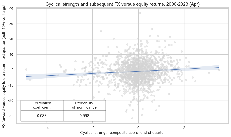
crx.reg_scatter(
    labels=False,
    coef_box="lower left",
    # separator=2011,
    #     xlab="",
    #     ylab="",
    #     title="",
    size=(10, 6),
    prob_est="map",
)

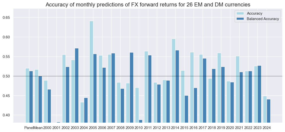
Accuracy and correlation check

dix = dict_fxeq_rf

sig = dix["sig"]
rivs = dix["rivs"]
targ = dix["targ"]
cidx = dix["cidx"]
blax = dix["black"]

srr = mss.SignalReturnRelations(
    dfx,
    cids=cidx,
    sigs=[sig] + rivs,
    rets=targ,
    freqs="M",
    start="2000-01-01",
    blacklist=blax,
)

dix["srr"] = srr

dix = dict_fxeq_rf
srrx = dix["srr"]
display(srrx.summary_table().astype("float").round(3))

	accuracy	bal_accuracy	pos_sigr	pos_retr	pos_prec	neg_prec	pearson	pearson_pval	kendall	kendall_pval	auc
M: CSGILvBM_ZC/last => FXvEQXR	0.520	0.513	0.414	0.460	0.475	0.551	0.079	0.000	0.041	0.000	0.513
Mean years	0.517	0.500	0.423	0.461	0.463	0.538	0.047	0.392	0.015	0.487	0.500
Positive ratio	0.560	0.560	0.360	0.240	0.360	0.760	0.680	0.440	0.480	0.360	0.560
Mean cids	0.518	0.505	0.424	0.462	0.467	0.543	0.055	0.334	0.028	0.434	0.505
Positive ratio	0.733	0.533	0.267	0.133	0.200	0.800	0.733	0.533	0.667	0.467	0.533

dix = dict_fxeq_rf
srrx = dix["srr"]
display(srrx.signals_table().sort_index().astype("float").round(3))

				accuracy	bal_accuracy	pos_sigr	pos_retr	pos_prec	neg_prec	pearson	pearson_pval	kendall	kendall_pval	auc
Return	Signal	Frequency	Aggregation
FXvEQXR	CSGILvBM_ZC	M	last	0.520	0.513	0.414	0.460	0.475	0.551	0.079	0.000	0.041	0.000	0.513
	CSGIvBM_ZC	M	last	0.504	0.500	0.447	0.459	0.459	0.541	0.058	0.000	0.027	0.014	0.500
	CSGLvBM_ZC	M	last	0.518	0.513	0.432	0.460	0.474	0.551	0.062	0.000	0.039	0.000	0.512
	CSGvBM_ZC	M	last	0.506	0.503	0.460	0.459	0.463	0.543	0.030	0.067	0.014	0.204	0.503
	CSILvBM_ZC	M	last	0.519	0.514	0.435	0.460	0.476	0.553	0.083	0.000	0.046	0.000	0.514
	CSIvBM_ZC	M	last	0.512	0.508	0.452	0.457	0.466	0.551	0.052	0.001	0.031	0.005	0.508
	CSLvBM_ZC	M	last	0.530	0.526	0.436	0.459	0.488	0.563	0.066	0.000	0.042	0.000	0.525

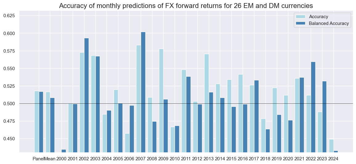
dix = dict_fxeq_rf
srrx = dix["srr"]
srrx.accuracy_bars(
    type="years",
    title="Accuracy of monthly predictions of FX forward returns for 26 EM and DM currencies",
    size=(14, 6),
)

Naive PnL

dix = dict_fxeq_rf

sigx = [dix["sig"]] + dix["rivs"]
targ = dix["targ"]
cidx = dix["cidx"]
blax = dix["black"]

naive_pnl = msn.NaivePnL(
    dfx,
    ret=targ,
    sigs=sigx,
    cids=cidx,
    start="2000-01-01",
    blacklist=blax,
    bms=["USD_EQXR_NSA"],
)

for sig in sigx:
    naive_pnl.make_pnl(
        sig,
        sig_neg=False,
        sig_op="zn_score_pan",
        thresh=3,
        rebal_freq="monthly",
        vol_scale=10,
        rebal_slip=1,
        pnl_name=sig + "_PZN",
    )

for sig in sigx:
    naive_pnl.make_pnl(
        sig,
        sig_neg=False,
        sig_op="binary",
        thresh=3,
        rebal_freq="monthly",
        vol_scale=10,
        rebal_slip=1,
        pnl_name=sig + "_BIN",
    )

naive_pnl.make_long_pnl(vol_scale=10, label="Long only")
dix["pnls"] = naive_pnl

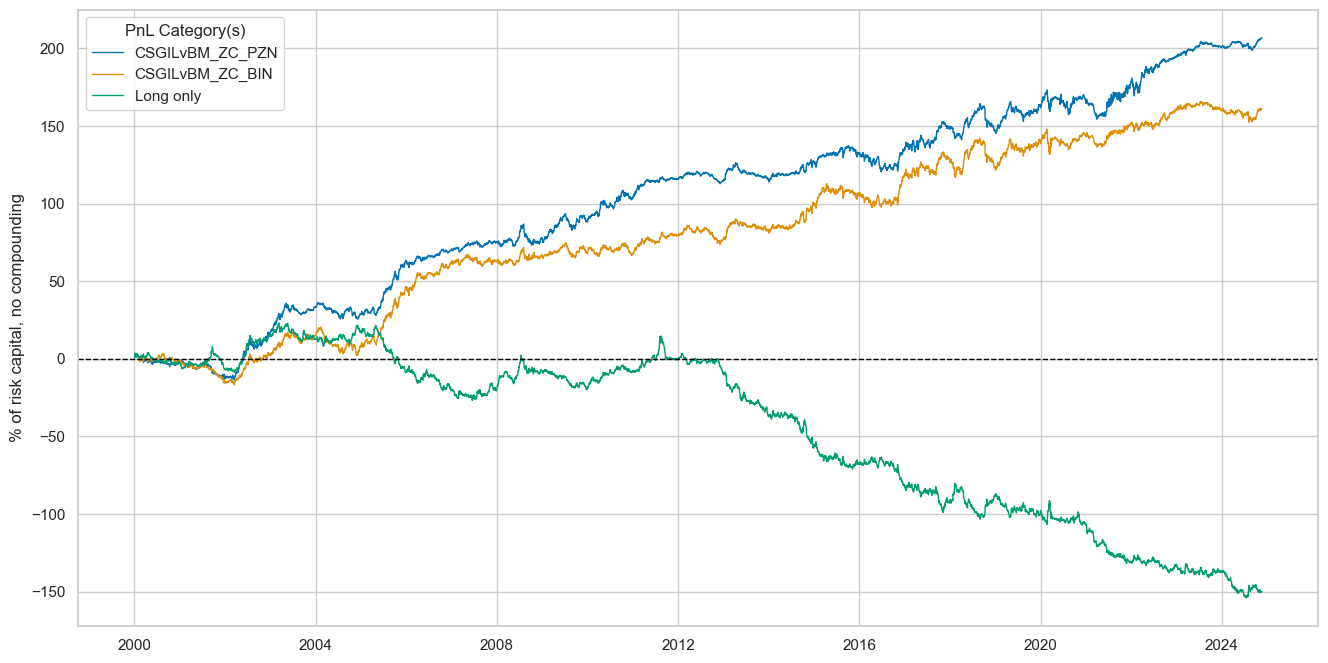
dix = dict_fxeq_rf

sigx = dix["sig"]
naive_pnl = dix["pnls"]
pnls = [sigx + x for x in ["_PZN", "_BIN"]] + ["Long only"]

naive_pnl.plot_pnls(
    pnl_cats=pnls,
    pnl_cids=["ALL"],
    start="2000-01-01",
    title=None,
    xcat_labels=None,
    figsize=(16, 8),
)

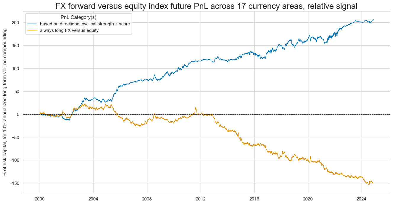
dix = dict_fxeq_rf

sigx = dix["sig"]
naive_pnl = dix["pnls"]
pnls = [sigx + "_PZN"] + ["Long only"]

dict_labels={"CSGILvBM_ZC_PZN": "based on directional cyclical strength z-score",
         "Long only": "always long FX versus equity"}

naive_pnl.plot_pnls(
    pnl_cats=pnls,
    pnl_cids=["ALL"],
    start="2000-01-01",
    title="FX forward versus equity index future PnL across 17 currency areas, relative signal",
    xcat_labels=dict_labels,
    ylab="% of risk capital, for 10% annualized long-term vol, no compounding",
    figsize=(16, 8),
)

dix = dict_fxeq_rf

sigx = dix["rivs"]
naive_pnl = dix["pnls"]
pnls = [sig + "_PZN" for sig in sigx]

naive_pnl.plot_pnls(
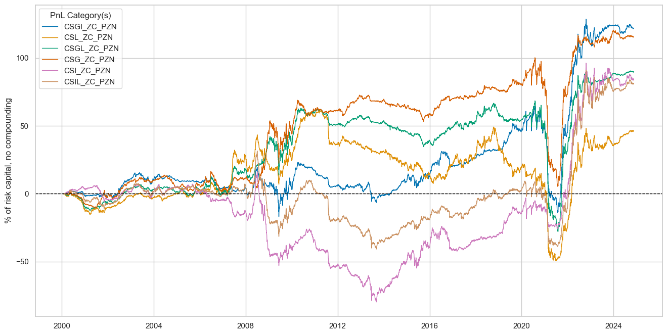
    pnl_cats=pnls,
    pnl_cids=["ALL"],
    start="2000-01-01",
    title=None,
    xcat_labels=None,
    figsize=(16, 8),
)

dix = dict_fxeq_rf

sigx = [dix["sig"]] + dix["rivs"]
naive_pnl = dix["pnls"]
pnls = [sig + type for sig in sigx for type in ["_PZN", "_BIN"]]

df_eval = naive_pnl.evaluate_pnls(
    pnl_cats=pnls,
    pnl_cids=["ALL"],
    start="2000-01-01",
)
display(df_eval.transpose())

	Return %	St. Dev. %	Sharpe Ratio	Sortino Ratio	Max 21-Day Draw %	Max 6-Month Draw %	Peak to Trough Draw %	Top 5% Monthly PnL Share	USD_EQXR_NSA correl	Traded Months
xcat
CSGILvBM_ZC_PZN	8.334418	10.0	0.833442	1.200683	-13.459492	-15.37297	-19.140221	0.544992	0.053613	298
CSGvBM_ZC_PZN	3.633139	10.0	0.363314	0.518486	-12.631551	-28.83066	-48.408873	1.121046	0.027406	298
CSGIvBM_ZC_PZN	6.38599	10.0	0.638599	0.919681	-10.220062	-20.709122	-36.673399	0.722807	0.087613	298
CSIvBM_ZC_PZN	5.946811	10.0	0.594681	0.850107	-13.722564	-26.15678	-51.667236	0.776585	0.081429	298
CSILvBM_ZC_PZN	8.530024	10.0	0.853002	1.231267	-15.410937	-11.863888	-22.370403	0.53846	0.044535	298
CSLvBM_ZC_PZN	7.094953	10.0	0.709495	1.03636	-14.434188	-19.075401	-29.061787	0.697287	-0.021247	298
CSGLvBM_ZC_PZN	7.195167	10.0	0.719517	1.044721	-12.642724	-23.13424	-25.77028	0.6325	0.005897	298
CSGILvBM_ZC_BIN	6.497507	10.0	0.649751	0.92958	-14.345262	-17.811849	-20.399282	0.702889	0.076423	298
CSGvBM_ZC_BIN	4.76715	10.0	0.476715	0.694914	-12.277093	-20.541087	-24.804862	0.98014	-0.003623	298
CSGIvBM_ZC_BIN	2.422004	10.0	0.2422	0.339401	-12.81974	-21.379071	-54.877378	1.784931	0.068329	298
CSIvBM_ZC_BIN	3.401567	10.0	0.340157	0.470308	-16.153116	-30.66803	-53.615872	1.214478	0.094164	298
CSILvBM_ZC_BIN	6.30651	10.0	0.630651	0.895957	-14.510664	-17.811018	-21.484719	0.642422	0.083834	298
CSLvBM_ZC_BIN	7.564915	10.0	0.756491	1.096419	-14.209912	-13.521302	-20.40971	0.638837	0.034001	298
CSGLvBM_ZC_BIN	6.013909	10.0	0.601391	0.856516	-13.891357	-21.967663	-30.864419	0.741706	0.011181	298

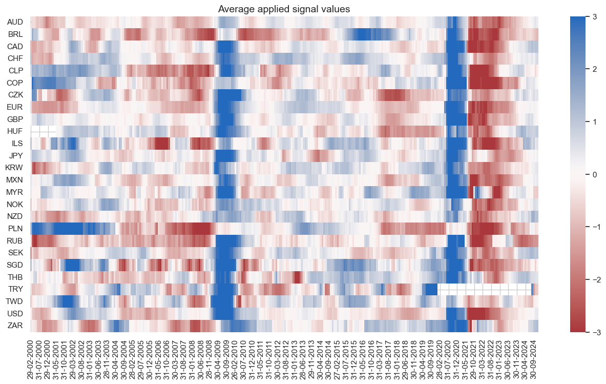
dix = dict_fxeq_rf
sig = dix["sig"]
naive_pnl = dix["pnls"]

naive_pnl.signal_heatmap(
    pnl_name=sig + "_PZN", freq="m", start="2000-01-01", figsize=(16, 5)
)

FX versus IRS strategy (relative features)

Specs and panel test

sigs = cs_rel
ms = "CSGILvBM_ZC"  # main signal
oths = list(set(sigs) - set([ms]))  # other signals

targ = "FXvDU05XR"
cidx = msm.common_cids(dfx, sigs + [targ])
cidx = list(set(cidx_fxdu) & set(cidx))
dict_fxdu_rf = {
    "sig": ms,
    "rivs": oths,
    "targ": targ,
    "cidx": cidx,
    "black": fxblack,
    "srr": None,
    "pnls": None,
}

dix = dict_fxdu_rf

sig = dix["sig"]
targ = dix["targ"]
cidx = dix["cidx"]
blax = dix["black"]

crx = msp.CategoryRelations(
    dfx,
    xcats=[sig, targ],
    cids=cidx,
    freq="Q",  # quarterly frequency allows for policy inertia
    lag=1,
    xcat_aggs=["last", "sum"],
    start="2000-01-01",
    blacklist=blax,
    xcat_trims=[None, None],
)
crx.reg_scatter(
    labels=False,
    coef_box="lower left",
    xlab="Cyclical strength composite score versus benchmark currency area, end of quarter",
    ylab="FX foward return versus 5-year IRS return, volatility neutral, next quarter",
    title="Relative cyclical strength and subsequent FX versus IRS returns, 2000-2023 (Apr)",
    size=(10, 6),
    prob_est="map",
)

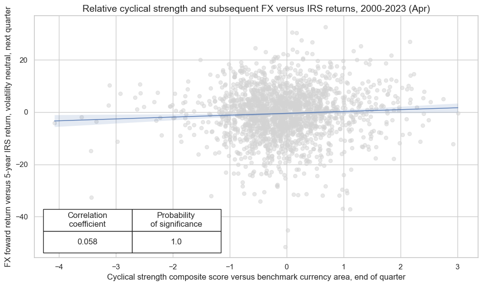
Accuracy and correlation check

dix = dict_fxdu_rf

sig = dix["sig"]
rivs = dix["rivs"]
targ = dix["targ"]
cidx = dix["cidx"]
blax = dix["black"]

srr = mss.SignalReturnRelations(
    dfx,
    cids=cidx,
    sigs=[sig] + rivs,
    rets=targ,
    freqs="M",
    start="2000-01-01",
    blacklist=blax,
)

dix["srr"] = srr

dix = dict_fxdu_rf
srrx = dix["srr"]
display(srrx.summary_table().astype("float").round(3))

	accuracy	bal_accuracy	pos_sigr	pos_retr	pos_prec	neg_prec	pearson	pearson_pval	kendall	kendall_pval	auc
M: CSGILvBM_ZC/last => FXvDU05XR	0.522	0.523	0.440	0.501	0.526	0.519	0.053	0.000	0.033	0.000	0.522
Mean years	0.522	0.520	0.442	0.495	0.510	0.529	0.068	0.395	0.040	0.379	0.518
Positive ratio	0.560	0.720	0.400	0.440	0.480	0.640	0.800	0.560	0.720	0.520	0.720
Mean cids	0.523	0.522	0.448	0.503	0.528	0.517	0.036	0.433	0.029	0.391	0.521
Positive ratio	0.783	0.783	0.348	0.609	0.696	0.609	0.609	0.391	0.609	0.435	0.783

dix = dict_fxdu_rf
srrx = dix["srr"]
display(srrx.signals_table().sort_index().astype("float").round(3))

				accuracy	bal_accuracy	pos_sigr	pos_retr	pos_prec	neg_prec	pearson	pearson_pval	kendall	kendall_pval	auc
Return	Signal	Frequency	Aggregation
FXvDU05XR	CSGILvBM_ZC	M	last	0.522	0.523	0.440	0.501	0.526	0.519	0.053	0.000	0.033	0.000	0.522
	CSGIvBM_ZC	M	last	0.508	0.508	0.462	0.502	0.511	0.505	0.047	0.001	0.025	0.006	0.508
	CSGLvBM_ZC	M	last	0.517	0.517	0.456	0.501	0.520	0.515	0.036	0.008	0.025	0.005	0.517
	CSGvBM_ZC	M	last	0.504	0.504	0.462	0.502	0.506	0.502	0.021	0.114	0.008	0.394	0.504
	CSILvBM_ZC	M	last	0.521	0.521	0.460	0.499	0.522	0.520	0.054	0.000	0.037	0.000	0.521
	CSIvBM_ZC	M	last	0.510	0.510	0.475	0.499	0.510	0.511	0.039	0.005	0.026	0.005	0.510
	CSLvBM_ZC	M	last	0.522	0.522	0.443	0.499	0.523	0.521	0.037	0.006	0.029	0.002	0.521

dix = dict_fxdu_rf
srrx = dix["srr"]
srrx.accuracy_bars(
    type="years",
    # title="Accuracy of monthly predictions of FX forward returns for 26 EM and DM currencies",
    size=(14, 6),
)

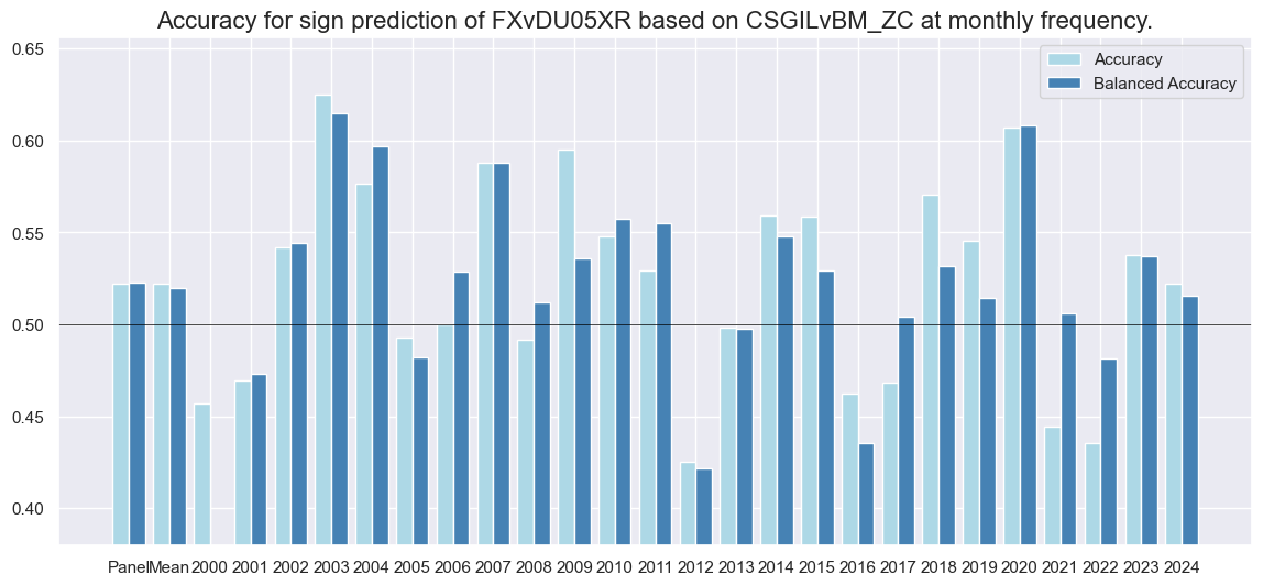
Naive PnL

dix = dict_fxdu_rf

sigx = [dix["sig"]] + dix["rivs"]
targ = dix["targ"]
cidx = dix["cidx"]
blax = dix["black"]

naive_pnl = msn.NaivePnL(
    dfx,
    ret=targ,
    sigs=sigx,
    cids=cidx,
    start="2000-01-01",
    blacklist=blax,
    bms=["USD_EQXR_NSA"],
)

for sig in sigx:
    naive_pnl.make_pnl(
        sig,
        sig_neg=False,
        sig_op="zn_score_pan",
        thresh=3,
        rebal_freq="monthly",
        vol_scale=10,
        rebal_slip=1,
        pnl_name=sig + "_PZN",
    )

for sig in sigx:
    naive_pnl.make_pnl(
        sig,
        sig_neg=False,
        sig_op="binary",
        thresh=3,
        rebal_freq="monthly",
        vol_scale=10,
        rebal_slip=1,
        pnl_name=sig + "_BIN",
    )

naive_pnl.make_long_pnl(vol_scale=10, label="Long only")
dix["pnls"] = naive_pnl

dix = dict_fxdu_rf

sigx = dix["sig"]
naive_pnl = dix["pnls"]
pnls = [sigx + x for x in ["_PZN", "_BIN"]] + ["Long only"]

naive_pnl.plot_pnls(
    pnl_cats=pnls,
    pnl_cids=["ALL"],
    start="2000-01-01",
    title=None,
    xcat_labels=None,
    figsize=(16, 8),
)

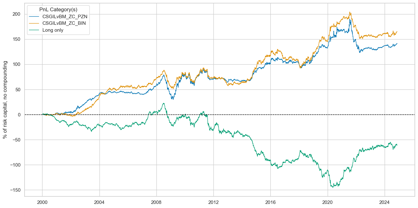
dix = dict_fxdu_rf

sigx = dix["sig"]
naive_pnl = dix["pnls"]
pnls = [sigx + "_PZN"] + ["Long only"]

dict_labels={"CSGILvBM_ZC_PZN": "based on cyclical strength z-score",
         "Long only": "always long FX forward and paying 5-year IRS yields"}

naive_pnl.plot_pnls(
    pnl_cats=pnls,
    pnl_cids=["ALL"],
    start="2000-01-01",
    title="FX versus duration PnL across 23 markets",
    xcat_labels=dict_labels,
    ylab="% of risk capital, for 10% annualized long-term vol, no compounding",
    figsize=(16, 8),
)

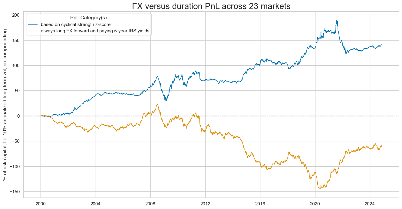
dix = dict_fxdu_rf

sigx = dix["rivs"]
naive_pnl = dix["pnls"]
pnls = [sig + "_PZN" for sig in sigx]

naive_pnl.plot_pnls(
    pnl_cats=pnls,
    pnl_cids=["ALL"],
    start="2000-01-01",
    title=None,
    xcat_labels=None,
    figsize=(16, 8),
)

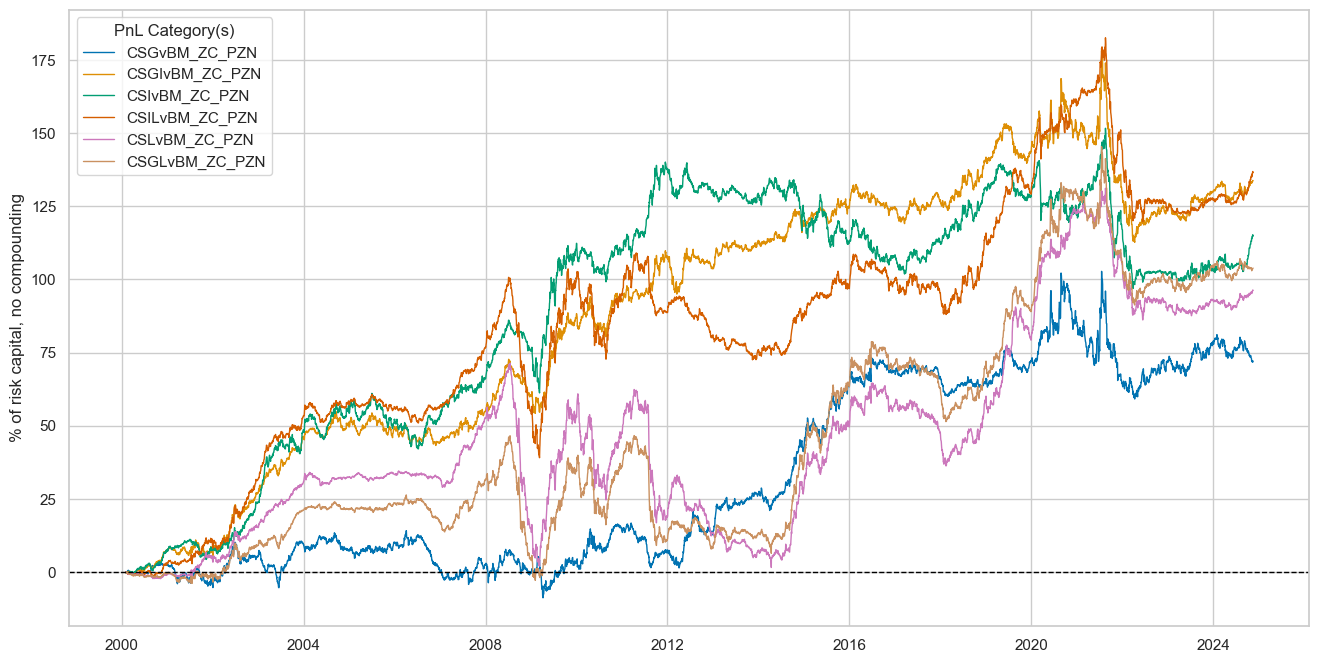
dix = dict_fxdu_rf

sigx = [dix["sig"]] + dix["rivs"]
naive_pnl = dix["pnls"]
pnls = [sig + type for sig in sigx for type in ["_PZN", "_BIN"]]

df_eval = naive_pnl.evaluate_pnls(
    pnl_cats=pnls,
    pnl_cids=["ALL"],
    start="2000-01-01",
)
display(df_eval.transpose())

	Return %	St. Dev. %	Sharpe Ratio	Sortino Ratio	Max 21-Day Draw %	Max 6-Month Draw %	Peak to Trough Draw %	Top 5% Monthly PnL Share	USD_EQXR_NSA correl	Traded Months
xcat
CSGILvBM_ZC_PZN	5.705776	10.0	0.570578	0.841965	-22.742112	-57.708844	-66.935626	1.002108	0.077799	298
CSGvBM_ZC_PZN	2.908389	10.0	0.290839	0.429563	-19.431038	-37.871655	-43.634825	1.74691	-0.026702	298
CSGIvBM_ZC_PZN	5.396073	10.0	0.539607	0.795309	-24.574693	-55.056114	-65.397084	0.974997	0.027617	298
CSIvBM_ZC_PZN	4.632813	10.0	0.463281	0.663906	-20.566443	-47.909548	-54.772466	1.08541	0.063032	298
CSILvBM_ZC_PZN	5.509477	10.0	0.550948	0.793448	-21.949948	-54.15788	-62.824813	1.030086	0.108625	298
CSLvBM_ZC_PZN	3.884578	10.0	0.388458	0.550726	-25.688218	-61.550766	-69.792614	1.477448	0.110023	298
CSGLvBM_ZC_PZN	4.189499	10.0	0.41895	0.620696	-22.161625	-45.352959	-54.102618	1.465566	0.063255	298
CSGILvBM_ZC_BIN	6.658925	10.0	0.665892	0.979691	-16.576618	-40.926422	-53.786432	0.800388	0.0475	298
CSGvBM_ZC_BIN	2.780417	10.0	0.278042	0.406489	-13.144493	-21.568452	-34.890465	1.921451	-0.039457	298
CSGIvBM_ZC_BIN	2.679043	10.0	0.267904	0.380338	-17.183719	-39.939308	-58.40352	1.742986	0.012735	298
CSIvBM_ZC_BIN	2.239245	10.0	0.223924	0.313177	-19.258438	-33.219595	-73.477535	2.01483	0.052814	298
CSILvBM_ZC_BIN	5.210797	10.0	0.52108	0.752131	-19.915943	-42.402214	-56.886312	1.005219	0.08399	298
CSLvBM_ZC_BIN	4.903122	10.0	0.490312	0.714716	-19.219114	-46.212205	-50.655189	1.224319	0.059743	298
CSGLvBM_ZC_BIN	3.691029	10.0	0.369103	0.536085	-24.455219	-45.540782	-53.794755	1.622247	0.044212	298

dix = dict_fxdu_rf
sig = dix["sig"]
naive_pnl = dix["pnls"]

naive_pnl.signal_heatmap(
    pnl_name=sig + "_PZN", freq="m", start="2000-01-01", figsize=(16, 6)
)

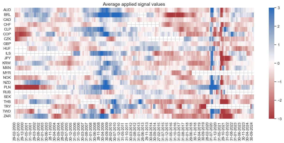
IRS curve flattening strategy

Specs and panel test

sigs = cs_dir
ms = "CSGIL_ZC"  # main signal
oths = list(set(sigs) - set([ms]))  # other signals

targ = "DU05v02XR"
cidx = msm.common_cids(dfx, sigs + [targ])
cidx = list(set(cidx_du52) & set(cidx))

dict_du52 = {
    "sig": ms,
    "rivs": oths,
    "targ": targ,
    "cidx": cidx,
    "black": dublack,
    "srr": None,
    "pnls": None,
}

dix = dict_du52

sig = dix["sig"]
targ = dix["targ"]
cidx = dix["cidx"]
blax = dix["black"]

crx = msp.CategoryRelations(
    dfx,
    xcats=[sig, targ],
    cids=cidx,
    freq="Q",
    lag=1,
    xcat_aggs=["last", "sum"],
    start="2000-01-01",
    blacklist=blax,
    xcat_trims=[None, None],
)
crx.reg_scatter(
    labels=False,
    coef_box="lower left",
    xlab="Cyclical strength composite score, end of quarter",
    ylab="IRS curve 2s-5s flattening return next quarter",
    title="Cyclical strength and subsequent IRS flattening returns, 2000-2023 (Apr)",
    size=(10, 6),
    prob_est="map",
)

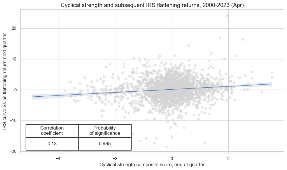
Accuracy and correlation check

dix = dict_du52

sig = dix["sig"]
rivs = dix["rivs"]
targ = dix["targ"]
cidx = dix["cidx"]
blax = dix["black"]

srr = mss.SignalReturnRelations(
    dfx,
    cids=cidx,
    sigs=[sig] + rivs,
    rets=targ,
    freqs="M",
    start="2000-01-01",
    blacklist=blax,
)

dix["srr"] = srr

dix = dict_du52
srrx = dix["srr"]
display(srrx.summary_table().astype("float").round(3))

	accuracy	bal_accuracy	pos_sigr	pos_retr	pos_prec	neg_prec	pearson	pearson_pval	kendall	kendall_pval	auc
M: CSGIL_ZC/last => DU05v02XR	0.534	0.534	0.498	0.517	0.551	0.516	0.091	0.000	0.053	0.000	0.534
Mean years	0.531	0.517	0.504	0.517	0.531	0.503	0.030	0.362	0.028	0.391	0.516
Positive ratio	0.760	0.680	0.520	0.560	0.680	0.480	0.640	0.440	0.640	0.440	0.680
Mean cids	0.533	0.537	0.502	0.515	0.548	0.525	0.102	0.261	0.059	0.284	0.536
Positive ratio	0.846	0.846	0.538	0.654	0.808	0.615	0.885	0.769	0.846	0.692	0.846

dix = dict_du52
srrx = dix["srr"]
display(srrx.signals_table().sort_index().astype("float").round(3))

				accuracy	bal_accuracy	pos_sigr	pos_retr	pos_prec	neg_prec	pearson	pearson_pval	kendall	kendall_pval	auc
Return	Signal	Frequency	Aggregation
DU05v02XR	CSGIL_ZC	M	last	0.534	0.534	0.498	0.517	0.551	0.516	0.091	0.000	0.053	0.000	0.534
	CSGI_ZC	M	last	0.534	0.536	0.438	0.517	0.558	0.515	0.089	0.000	0.057	0.000	0.536
	CSGL_ZC	M	last	0.537	0.536	0.538	0.517	0.550	0.521	0.099	0.000	0.059	0.000	0.535
	CSG_ZC	M	last	0.529	0.531	0.451	0.517	0.551	0.511	0.099	0.000	0.065	0.000	0.531
	CSIL_ZC	M	last	0.520	0.520	0.516	0.518	0.537	0.502	0.048	0.000	0.025	0.002	0.520
	CSI_ZC	M	last	0.511	0.513	0.464	0.518	0.532	0.493	0.024	0.051	0.014	0.084	0.513
	CSL_ZC	M	last	0.530	0.527	0.623	0.518	0.538	0.516	0.057	0.000	0.033	0.000	0.525

dix = dict_du52
srrx = dix["srr"]
srrx.accuracy_bars(
    type="years",
    # title="",
    size=(14, 6),
)

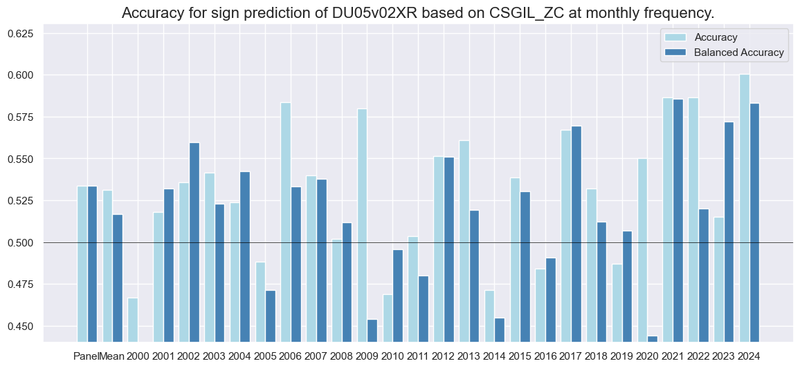
Naive PnL

dix = dict_du52

sigx = [dix["sig"]] + dix["rivs"]
targ = dix["targ"]
cidx = dix["cidx"]
blax = dix["black"]

naive_pnl = msn.NaivePnL(
    dfx,
    ret=targ,
    sigs=sigx,
    cids=cidx,
    start="2000-01-01",
    blacklist=blax,
    bms=["USD_EQXR_NSA", "USD_DU05YXR_VT10"],
)

for sig in sigx:
    naive_pnl.make_pnl(
        sig,
        sig_neg=False,
        sig_op="zn_score_pan",
        thresh=3,
        rebal_freq="monthly",
        vol_scale=10,
        rebal_slip=1,
        pnl_name=sig + "_PZN",
    )

for sig in sigx:
    naive_pnl.make_pnl(
        sig,
        sig_neg=False,
        sig_op="binary",
        thresh=3,
        rebal_freq="monthly",
        vol_scale=10,
        rebal_slip=1,
        pnl_name=sig + "_BIN",
    )

naive_pnl.make_long_pnl(vol_scale=10, label="Long only")
dix["pnls"] = naive_pnl

dix = dict_du52

sigx = dix["sig"]
naive_pnl = dix["pnls"]
pnls = [sigx + x for x in ["_PZN", "_BIN"]] + ["Long only"]

naive_pnl.plot_pnls(
    pnl_cats=pnls,
    pnl_cids=["ALL"],
    start="2000-01-01",
    title=None,
    xcat_labels=None,
    figsize=(16, 8),
)

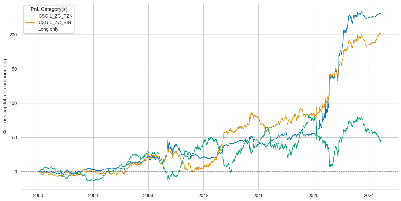
dix = dict_du52

sigx = dix["sig"]
naive_pnl = dix["pnls"]
pnls = [sigx + "_PZN"] + ["Long only"]

dict_labels={"CSGIL_ZC_PZN": "based on negative of cyclical strength z-score",
             "Long only": "always long 5-year versus 2-year, volatility neutral"}


naive_pnl.plot_pnls(
    pnl_cats=pnls,
    pnl_cids=["ALL"],
    start="2000-01-01",
    title="IRS curve flattening PnL across 25 markets",
    xcat_labels=dict_labels,
    ylab="% of risk capital, for 10% annualized long-term vol, no compounding",
    figsize=(16, 8),
)

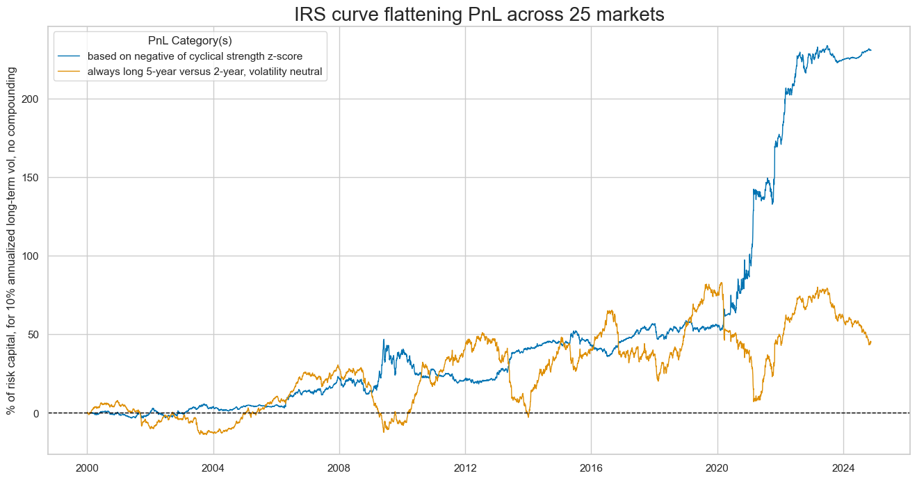
dix = dict_du52

sigx = dix["rivs"]
naive_pnl = dix["pnls"]
pnls = [sig + "_PZN" for sig in sigx]

naive_pnl.plot_pnls(
    pnl_cats=pnls,
    pnl_cids=["ALL"],
    start="2000-01-01",
    title=None,
    xcat_labels=None,
    figsize=(16, 8),
)

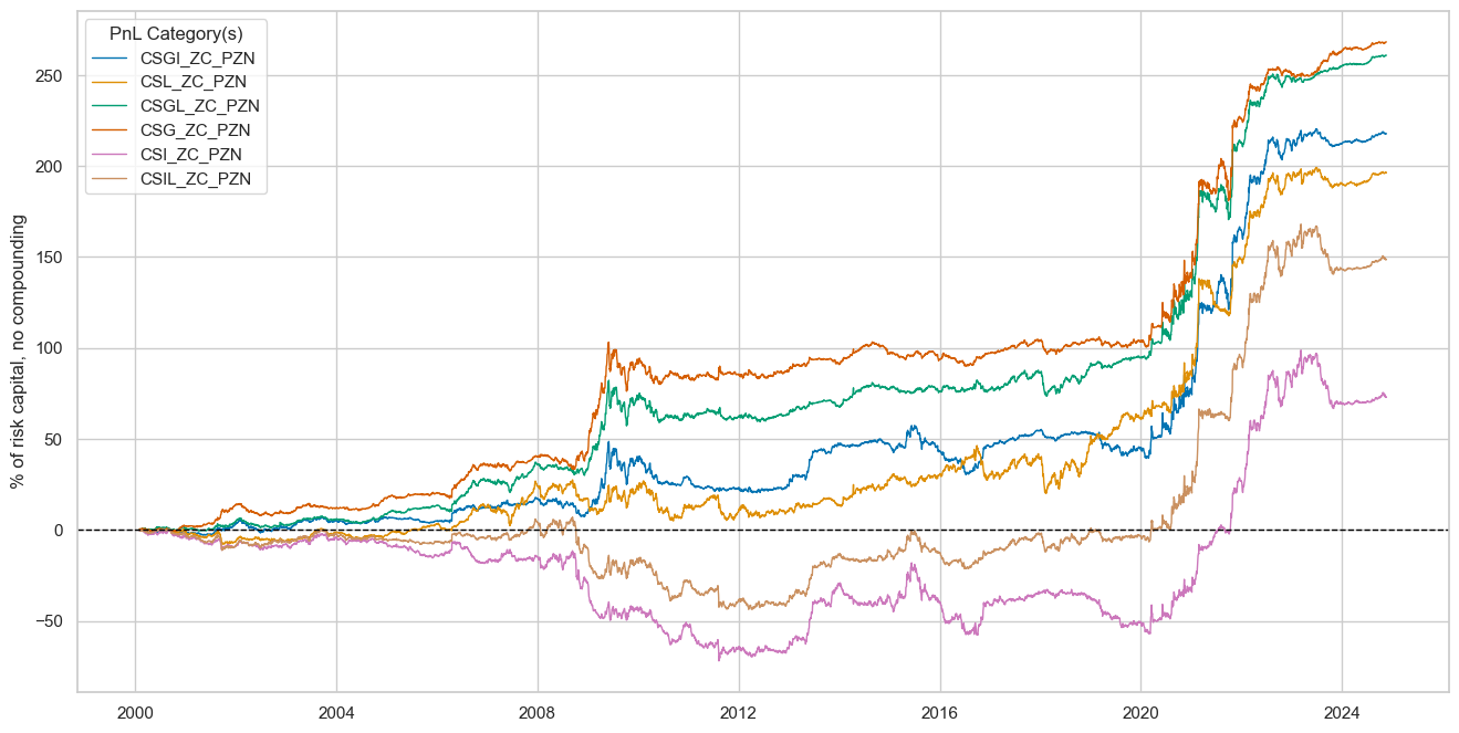
dix = dict_du52

sigx = [dix["sig"]] + dix["rivs"]
naive_pnl = dix["pnls"]
pnls = [sig + type for sig in sigx for type in ["_PZN", "_BIN"]]

df_eval = naive_pnl.evaluate_pnls(
    pnl_cats=pnls,
    pnl_cids=["ALL"],
    start="2000-01-01",
)
display(df_eval.transpose())

	Return %	St. Dev. %	Sharpe Ratio	Sortino Ratio	Max 21-Day Draw %	Max 6-Month Draw %	Peak to Trough Draw %	Top 5% Monthly PnL Share	USD_EQXR_NSA correl	USD_DU05YXR_VT10 correl	Traded Months
xcat
CSGIL_ZC_PZN	9.30828	10.0	0.930828	1.602482	-13.101565	-16.115859	-28.495641	0.958435	0.024137	-0.07648	298
CSGI_ZC_PZN	8.784759	10.0	0.878476	1.492628	-15.147253	-15.059561	-28.172829	1.011797	0.024483	-0.11011	298
CSL_ZC_PZN	7.924012	10.0	0.792401	1.276974	-19.557033	-19.692997	-26.066696	0.910919	0.01463	0.028277	298
CSGL_ZC_PZN	10.522971	10.0	1.052297	1.814258	-15.630049	-14.370811	-24.981082	0.813368	0.015456	-0.030921	298
CSG_ZC_PZN	10.818679	10.0	1.081868	1.871761	-18.94251	-13.683236	-26.986602	0.821327	0.011263	-0.065007	298
CSI_ZC_PZN	2.942892	10.0	0.294289	0.442672	-14.528025	-34.794992	-71.809352	2.469762	0.029264	-0.119609	298
CSIL_ZC_PZN	5.996261	10.0	0.599626	0.956262	-14.380579	-32.900758	-50.712404	1.355478	0.028083	-0.075213	298
CSGIL_ZC_BIN	8.106836	10.0	0.810684	1.274466	-14.06567	-23.065628	-37.894811	0.871917	0.027545	-0.067672	298
CSGI_ZC_BIN	9.015673	10.0	0.901567	1.434	-13.927554	-20.471159	-36.391596	0.828269	0.022031	-0.12981	298
CSL_ZC_BIN	7.523371	10.0	0.752337	1.14014	-17.111959	-21.624304	-24.576293	0.801078	0.013647	0.074663	298
CSGL_ZC_BIN	9.233738	10.0	0.923374	1.404978	-19.936405	-20.350348	-28.67883	0.729952	0.030338	0.02073	298
CSG_ZC_BIN	8.695058	10.0	0.869506	1.370465	-18.059032	-16.35807	-38.118483	0.820772	0.000064	-0.03682	298
CSI_ZC_BIN	3.008657	10.0	0.300866	0.447186	-12.71434	-32.241979	-69.227554	2.134317	0.036158	-0.153123	298
CSIL_ZC_BIN	5.50472	10.0	0.550472	0.846595	-13.614443	-32.006319	-61.122907	1.222398	0.021865	-0.094039	298

dix = dict_du52
sig = dix["sig"]
naive_pnl = dix["pnls"]

naive_pnl.signal_heatmap(
    pnl_name=sig + "_PZN", freq="m", start="2000-01-01", figsize=(16, 6)
)