Macro-aware equity-duration risk parity #
This notebook presents updated findings from the Macrosynergy post “Macro Factors of the Risk-Parity Trade,” originally published in November 2022 and revised in May 2025. The update focuses on three key enhancements:
-
Inclusion of pre-2000 history, now available for several major developed markets, enabling broader historical analysis.
-
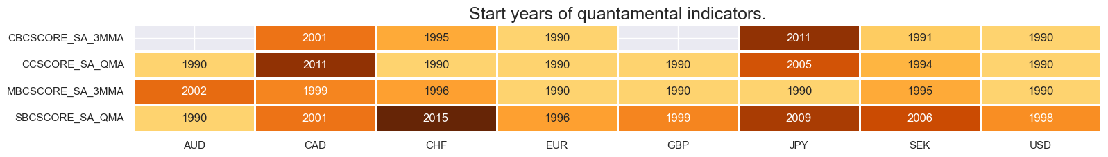
Integration of Macro-Quantamental Scorecards—concise, point-in-time visual summaries of economic conditions tailored to specific markets—currently available for fixed income, FX, and emerging market bonds.
-
Expanded set of overheating (or economic slack) indicators, introducing additional signals of macroeconomic pressure that influence asset returns and allocation decisions.
Risk parity positioning — balancing risk between equities and fixed income duration — has been a successful strategy over recent decades, largely supported by accommodative refinancing conditions and disinflationary trends. However, the macro environment is dynamic, and periods of economic overheating can challenge traditional risk-parity assumptions. We propose simple macro-quantamental strategies based on overheating indicators, which have historically shown strong correlations with risk-parity performance and could enhance returns even during the strategy’s “golden decades.”
This notebook provides the essential code to replicate the analysis discussed in the post and is structured into four main parts:
-
Packages and Data: Install libraries and retrieve JPMaQS data.
-
Transformations and Checks: Merge Germany–euro area data, apply 3MMA to quarterly tickers, and use OECD inflation MA as a proxy target for earlier periods.
-
Feature Engineering: Build thematic feature groups and perform preliminary analysis.
-
Target Returns: Conduct an initial exploration.
-
Value Checks: Backtest trading strategies aligned with economic overheating hypotheses.
While this notebook focuses on core developed markets and selected indicators, users are encouraged to adapt and extend the framework to other economies, financial returns, and research ideas. Good luck with your exploration!
Get packages and JPMaQS data #
import os
import pandas as pd

import macrosynergy.management as msm
import macrosynergy.panel as msp
import macrosynergy.signal as mss
import macrosynergy.pnl as msn
import macrosynergy.visuals as msv

from macrosynergy.management.utils import merge_categories
from macrosynergy.download import transform_to_qdf

from macrosynergy.download import JPMaQSDownload

import warnings

warnings.simplefilter("ignore")

import requests # for OECD API data
from io import StringIO # for OECD API data
JPMaQS indicators are retrieved via the J.P. Morgan DataQuery API, accessed through the macrosynergy package. Tickers are constructed by combining a currency area code (<cross_section>) and an indicator code (
JPMAQS,<cross_section>_<category>,<info>
), where
-
value: Latest indicator value -
eop_lag: Days since end of period -
mop_lag: Days since mean observation period -
grade: Quality metric of the observation
To download data, instantiate JPMaQSDownload from macrosynergy.download and call the download(tickers, start_date, metrics) method.For full details see the Macrosynergy GitHub documentation
#  DM currency area identifiers

cids = ["AUD", "CAD", "CHF", "DEM", "EUR", "GBP", "JPY", "SEK", "USD"] # includes DEM for extending EUR data to the early 1990s
cids_ll = ["AUD", "CAD", "CHF", "EUR", "GBP", "JPY", "SEK", "USD"]
# Category tickers

gdp = [
    "INTRGDPv5Y_NSA_P1M1ML12_3MMA",
    "RGDPTECHv5Y_SA_P1M1ML12_3MMA",
    "RGDP_SA_P1Q1QL4_20QMM",
] # growth indicators

cons = [
    "RPCONS_SA_P1M1ML12_3MMA",
    "RPCONS_SA_P1Q1QL4",
    "NRSALES_SA_P1M1ML12",
    "NRSALES_SA_P1M1ML12_3MMA",
    "NRSALES_SA_P1Q1QL4",
    "RRSALES_SA_P1M1ML12",
    "RRSALES_SA_P1M1ML12_3MMA",
    "RRSALES_SA_P1Q1QL4",
]  # consumption indicators

imports = [
   "IMPORTS_SA_P1M1ML12_3MMA",
]  #  foreign trade trend

demand = cons + imports

conf = [
    "MBCSCORE_SA_3MMA",
    "CBCSCORE_SA_3MMA",
    "CCSCORE_SA",
    "CCSCORE_SA_3MMA",
    "SBCSCORE_SA",
    "SBCSCORE_SA_3MMA",
]  # confidence scores

infl = [
    "CPIH_SA_P1M1ML12",
    "CPIH_SJA_P6M6ML6AR",
    "CPIC_SA_P1M1ML12",
    "CPIC_SJA_P6M6ML6AR",
    "INFTEFF_NSA"
]  # inflation indicators


macro = gdp + demand + conf + infl

markets = [
    "EQXR_NSA",
    "EQXR_VT10",
    "DU05YXR_NSA",
    "DU05YXR_VT10",
]

xcats = macro + markets

# Resultant tickers

tickers = [cid + "_" + xcat for cid in cids for xcat in xcats]
print(f"Maximum number of tickers is {len(tickers)}")
Maximum number of tickers is 243
#  Download series from J.P. Morgan DataQuery by tickers

start_date = "1990-01-01"

# Retrieve credentials
client_id: str = os.getenv("DQ_CLIENT_ID")
client_secret: str = os.getenv("DQ_CLIENT_SECRET")

with JPMaQSDownload(client_id=client_id, client_secret=client_secret) as dq:
    df = dq.download(
        tickers=tickers,
        start_date=start_date,
        suppress_warning=True,
        metrics=["value"],
        show_progress=True,
    )
Downloading data from JPMaQS.
Timestamp UTC:  2025-11-05 18:52:27
Connection successful!
Requesting data: 100%|██████████| 13/13 [00:02<00:00,  4.92it/s]
Downloading data: 100%|██████████| 13/13 [00:20<00:00,  1.60s/it]
Some expressions are missing from the downloaded data. Check logger output for complete list.
39 out of 243 expressions are missing. To download the catalogue of all available expressions and filter the unavailable expressions, set `get_catalogue=True` in the call to `JPMaQSDownload.download()`.
dfx = df.copy()
dfx.info()
<class 'pandas.core.frame.DataFrame'>
RangeIndex: 1603665 entries, 0 to 1603664
Data columns (total 4 columns):
 #   Column     Non-Null Count    Dtype
---  ------     --------------    -----
 0   real_date  1603665 non-null  datetime64[ns]
 1   cid        1603665 non-null  object
 2   xcat       1603665 non-null  object
 3   value      1603665 non-null  float64
dtypes: datetime64[ns](1), float64(1), object(2)
memory usage: 48.9+ MB
Transformations and availability checks #
Transformations #
# Combined Germany-euro area data

# Extract EUR and DEM data
dfx_eur = dfx[dfx["cid"] == "EUR"]
dfx_dem = dfx[dfx["cid"] == "DEM"]

# Merge EUR and DEM data on real-time dates and categories
dfx_dea = pd.merge(
    dfx_eur,
    dfx_dem,
    on=["real_date", "xcat"],
    suffixes=("_eur", "_dem"),  # labels duplicate columns
    how="outer"  # includes values of all EUR and DEM cases, even if missing values
)

# Merge values of EUR and DEM data, with EUR preferred if both are available
dfx_dea["cid"] = "EUR"
dfx_dea["value"] = dfx_dea["value_eur"].combine_first(dfx_dea["value_dem"])
dfx_dea = dfx_dea [list(dfx.columns)]

# Replace EUR and DEM with effective composite EUR
dfx = dfx[~dfx["cid"].isin(["EUR", "DEM"])]
dfx = msm.update_df(dfx, dfx_dea)
# Replace quarterly tickers with 3MMA tickers for convenience

dict_repl = {
    # Labor
    "RPCONS_SA_P1Q1QL4": "RPCONS_SA_P1M1ML12_3MMA",
    "RRSALES_SA_P1Q1QL4": "RRSALES_SA_P1M1ML12_3MMA",
    "NRSALES_SA_P1Q1QL4": "NRSALES_SA_P1M1ML12_3MMA",
}

# Ensure 'xcat' exists in dfx before replacement
if "xcat" in dfx.columns:
    dfx["xcat"] = dfx["xcat"].replace(dict_repl, regex=False)
else:
    print("Column 'xcat' not found in dfx.")
# Combine 3mma and quarterly series for confidence scores

survs = ["CC", "SBC"]
for surv in survs:
    new_cat = f"{surv}SCORE_SA_QMA"
    ordered_cats = [f"{surv}SCORE_SA_3MMA", f"{surv}SCORE_SA"]  # monthly if available
    dfa = merge_categories(dfx, ordered_cats, new_cat)
    dfx = msm.update_df(dfx, dfa)

confx = [
    "MBCSCORE_SA_3MMA",
    "CBCSCORE_SA_3MMA",
    "CCSCORE_SA_QMA",
    "SBCSCORE_SA_QMA",
]
Non-quantamental inflation targets #
We use OECD API to fetch 1985-2005 CPI data for selected countries. This is based on on a custum table created with the OECD data explore here
The table has been created as follows:
-
Define URL for OECD SDMX API.
-
Specifies the dataset (DSD_PRICES@DF_PRICES_ALL) and dimensions:
-
Countries: Australia, Canada, Germany, Japan, USA, Sweden, UK, Switzerland
-
Frequency: Annual (A)
-
Indicator: CPI year-on-year growth rate (GY)
-
Time Period: From 1985 onward
-
Format: CSV with labels (human-readable)
-
# Effective inflation benchmarks before inflation targets from the OECD

url = "https://sdmx.oecd.org/public/rest/data/OECD.SDD.TPS,DSD_PRICES@DF_PRICES_ALL,1.0/CHE+USA+GBR+SWE+JPN+DEU+CAN+AUS.A.N.CPI.PA._T.N.GY?startPeriod=1985&dimensionAtObservation=AllDimensions&format=csvfilewithlabels"

# Fetch data
response = requests.get(url)

# Read the CSV response into a pandas DataFrame
oecd = pd.read_csv(StringIO(response.text))

# Preview the data
print(oecd.head(2))
  STRUCTURE                                STRUCTURE_ID  \
0  DATAFLOW  OECD.SDD.TPS:DSD_PRICES@DF_PRICES_ALL(1.0)
1  DATAFLOW  OECD.SDD.TPS:DSD_PRICES@DF_PRICES_ALL(1.0)

                                      STRUCTURE_NAME ACTION REF_AREA  \
0  Consumer price indices (CPIs, HICPs), COICOP 1999      I      CHE
1  Consumer price indices (CPIs, HICPs), COICOP 1999      I      CHE

  Reference area FREQ Frequency of observation METHODOLOGY Methodology  ...  \
0    Switzerland    A                   Annual           N    National  ...
1    Switzerland    A                   Annual           N    National  ...

  OBS_STATUS Observation status UNIT_MULT Unit multiplier BASE_PER  \
0          A       Normal value       NaN             NaN      NaN
1          A       Normal value       NaN             NaN      NaN

  Base period DURABILITY Durability DECIMALS Decimals
0         NaN        NaN        NaN        2      Two
1         NaN        NaN        NaN        2      Two

[2 rows x 34 columns]
# Select and Clean Relevant Columns
oecde = (
    oecd[["REF_AREA", "TIME_PERIOD", "MEASURE", "OBS_VALUE"]]
    .sort_values(by=["REF_AREA", "TIME_PERIOD"])
    .reset_index(drop=True)
)
oecde["TIME_PERIOD"] = pd.to_datetime(oecde["TIME_PERIOD"].astype(str) + "-01-01")

# Map OECD Country Codes to JPMaQS Currency Codes
cid_mapping = {
    "AUS": "AUD",
    "CAN": "CAD",
    "CHE": "CHF",
    "DEU": "DEM",
    "GBR": "GBP",
    "JPN": "JPY",
    "SWE": "SEK",
    "USA": "USD",
}

oecde["REF_AREA"] = oecde["REF_AREA"].replace(cid_mapping)

# Map Column Names to JPMaQS format
xcat_mapping = {
    "MEASURE": "xcat",
    "REF_AREA": "cid",
    "TIME_PERIOD": "real_date",
    "OBS_VALUE": "value",
}

oecde = transform_to_qdf(oecde, mapping=xcat_mapping)

# Compute 5-year CPI moving average excluding current year
inteff_oecd = (
    oecde[oecde["xcat"] == "CPI"]
    .groupby("cid")
    .apply(
        lambda g: g.assign(
            value=g["value"].shift(1).rolling(window=5, min_periods=5).mean(),
            xcat="INFTEFF_OECD",
        )
    )
    .reset_index(drop=True)
    .dropna(subset=["value"])
)

# Append new series back to dataset
oecde = msm.update_df(oecde, inteff_oecd)
# build full grid of all available business days for each cid (for further forward-filling of annual OECD moving averages to JPMaQS daily format)
business_days = pd.date_range(start="1990-01-01", end="2025-05-14", freq="B")
cidx = oecde["cid"].unique()
full_grid = pd.MultiIndex.from_product(
[cids, business_days],
names=["cid", "real_date"]
).to_frame(index=False)
full_grid["xcat"] = "INFTEFF_OECD" # insert column xcat
oecde["real_date"] = pd.to_datetime(oecde["real_date"])
full_grid["real_date"] = pd.to_datetime(full_grid["real_date"])
# Merge the full (daily) grid with the oecde DataFrame (containing annual CPI moving averages)
merged = pd.merge(full_grid, oecde, on=["cid", "real_date", "xcat"], how="left")
merged = merged.sort_values(by=["cid", "real_date"])
merged["value"] = merged.groupby("cid")["value"].ffill()
filled_oecde = merged[["real_date", "cid", "xcat", "value"]].reset_index(drop=True)
# update dfx With Filled Daily filled OECD Data
dfx = msm.update_df(dfx, filled_oecde)
# Create "INFTEFF_BX" by prioritizing INFTEFF_NSA, fallback to INFTEFF_OECD
combined_cat = "INFTEFF_BX"
component_cats = ["INFTEFF_NSA", "INFTEFF_OECD"]
cids = list(map(str, cids)) # if cids exists but may contain non-strings
dfx = msm.update_df(
dfx,
merge_categories(dfx, component_cats, combined_cat, cids)
).reset_index(drop=True)
# Fill missing EUR data with DEM values for INFTEFF_BX
df_dem = dfx[(dfx["cid"] == "DEM") & (dfx["xcat"] == "INFTEFF_BX")].copy()
df_eur = dfx[(dfx["cid"] == "EUR") & (dfx["xcat"] == "INFTEFF_BX")].copy()
df_merged = pd.merge(
df_eur,
df_dem[["real_date", "value"]],
on="real_date",
how="outer",
suffixes=("_eur", "_dem")
)
# fill missing EUR values with DEM values
df_merged["value_combined"] = df_merged["value_eur"].combine_first(df_merged["value_dem"])
# Build updated EUR series with combined values
df_eur_filled = df_merged[["real_date", "value_combined"]].copy()
df_eur_filled["cid"] = "EUR"
df_eur_filled["xcat"] = "INFTEFF_BX"
df_eur_filled.rename(columns={"value_combined": "value"}, inplace=True)
# Drop old EUR version
dfx = dfx[~((dfx["cid"] == "EUR") & (dfx["xcat"] == "INFTEFF_BX"))]
# Append filled version
dfx = msm.update_df(dfx, df_eur_filled)
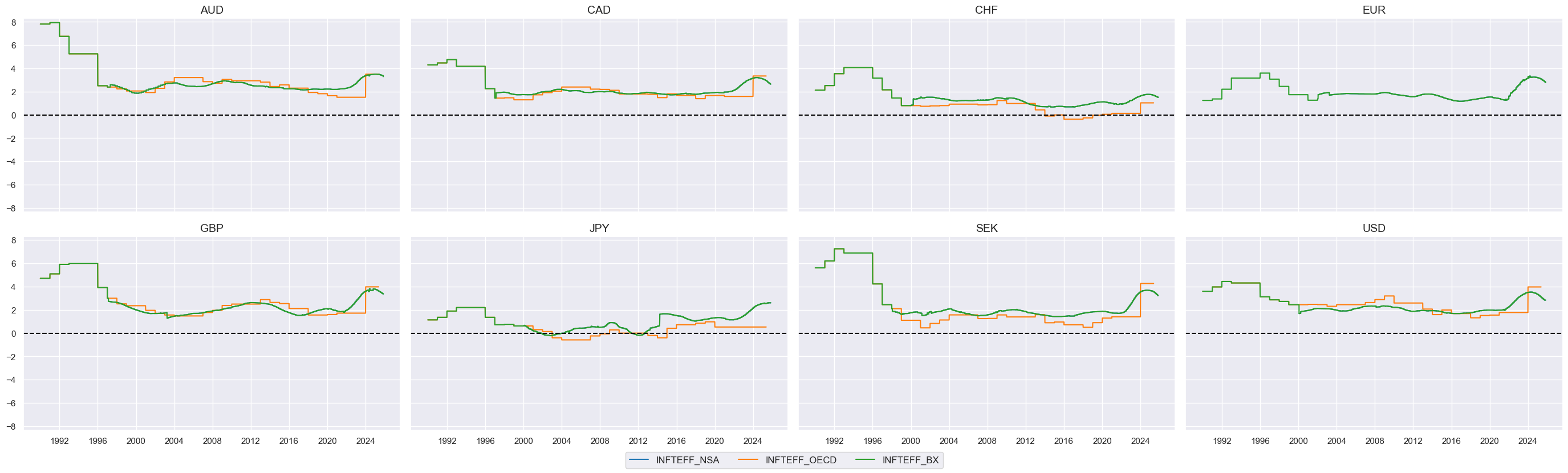
# visualize the timelines for the inflation targets
msp.view_timelines(
dfx,
start="1990-01-01",
ncol = 4,
cids=cids_ll,
xcats=["INFTEFF_NSA", "INFTEFF_OECD",
"INFTEFF_BX"
],
)
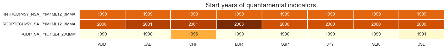
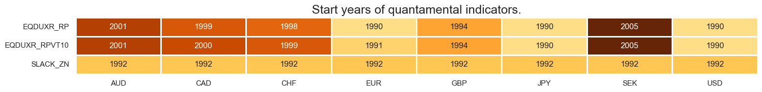
Availability of indicators after transformations #
xcatx = gdp
msm.check_availability(dfx, xcats = xcatx, cids=cids_ll, missing_recent=False)
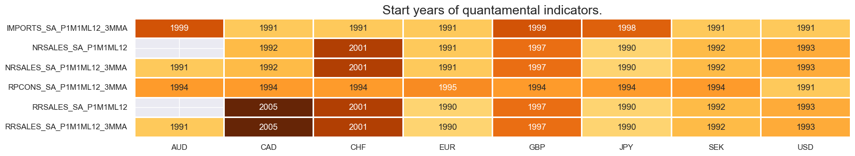
xcatx = demand
msm.check_availability(dfx, xcats = xcatx, cids=cids_ll, missing_recent=False)
xcatx = confx
msm.check_availability(dfx, xcats = xcatx, cids=cids_ll, missing_recent=False)
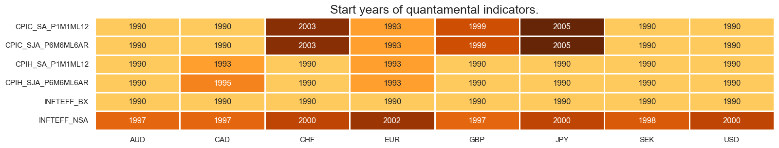
xcatx = infl + ["INFTEFF_BX"]
msm.check_availability(dfx, xcats = xcatx, cids=cids_ll, missing_recent=False)
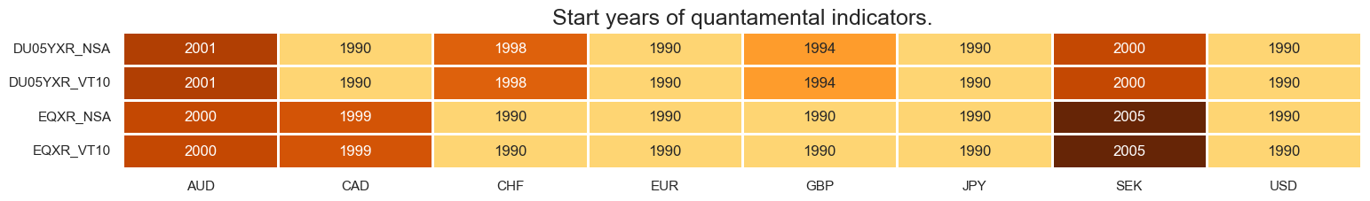
xcatx = markets
msm.check_availability(dfx, xcats = xcatx, cids=cids_ll, missing_recent=False)
Feature engineering and checks #
Excess inflation #
# Un-scored indicators and scored weights

dict_xinfl = {
    "XCPIH_SA_P1M1ML12": 0.5,
    "XCPIH_SJA_P6M6ML6AR": 0.5,
    "XCPIC_SA_P1M1ML12": 0.5,
    "XCPIC_SJA_P6M6ML6AR": 0.5,
}
# Excess inflation

xcatx = [key[1:] for key in dict_xinfl.keys()] # remove "X" prefix from xcat names in dict_xinfl

calcs = [f"X{xc} = {xc} - INFTEFF_BX" for xc in xcatx]

dfa = msp.panel_calculator(
    dfx,
    calcs=calcs,
    cids=cids,
)
dfx = msm.update_df(dfx, dfa)
# Normalization of excess inflation indicators
cidx = cids_ll
xcatx = list(dict_xinfl.keys())
sdate = "1990-01-01"
dfa = pd.DataFrame(columns=dfx.columns)
for xc in xcatx:
dfaa = msp.make_zn_scores(
dfx,
xcat=xc,
cids=cidx,
sequential=True,
min_obs=261 * 3,
neutral="zero",
pan_weight=1, # variance estimated based on panel and cross-sectional variation
thresh=3,
postfix="_ZN",
est_freq="m",
)
dfa = msm.update_df(dfa, dfaa)
dfx = msm.update_df(dfx, dfa)
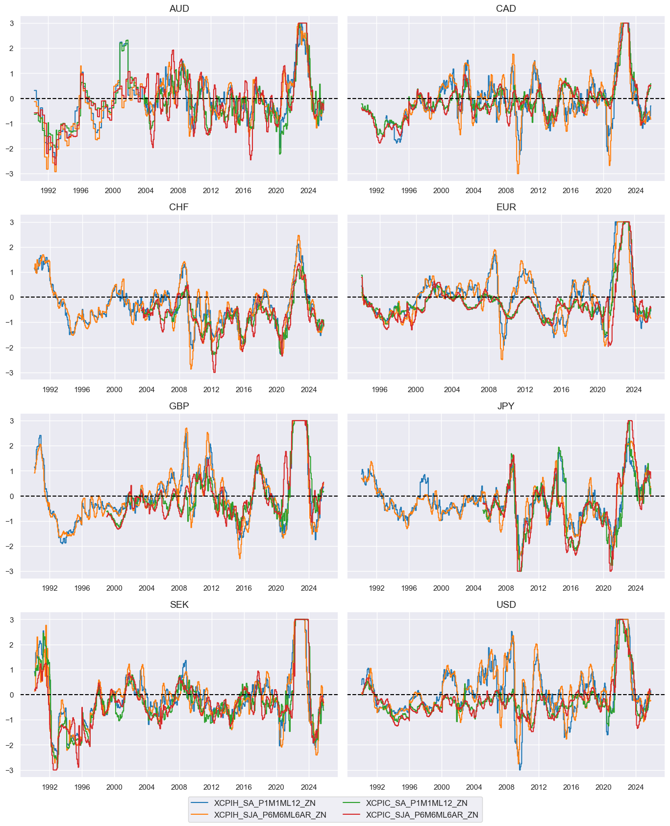
xinflz = [k + "_ZN" for k in list(dict_xinfl.keys())]
cidx = cids_ll
xcatx = xinflz

msp.view_timelines(
    dfx,
    xcats=xcatx,
    cids=cidx,
    ncol=2,
    start="1990-01-01",
    same_y=True,
    all_xticks=True,
)
# Weighted linear combination

cidx = cids_ll
xcatx = xinflz
weights = list(dict_xinfl.values())
czs = "XINFL"

dfa = msp.linear_composite(
    dfx,
    xcats=xcatx,
    cids=cidx,
    weights=weights,
    normalize_weights=True,
    complete_xcats=False,  # score works with what is available
    new_xcat=czs,
)
dfx = msm.update_df(dfx, dfa)

# Re-scoring

dfa = msp.make_zn_scores(
    dfx,
    xcat=czs,
    cids=cidx,
    sequential=True,
    min_obs=261 * 5,
    neutral="zero",
    pan_weight=1,
    thresh=3,
    postfix="_ZN",
    est_freq="m",
)
dfx = msm.update_df(dfx, dfa)
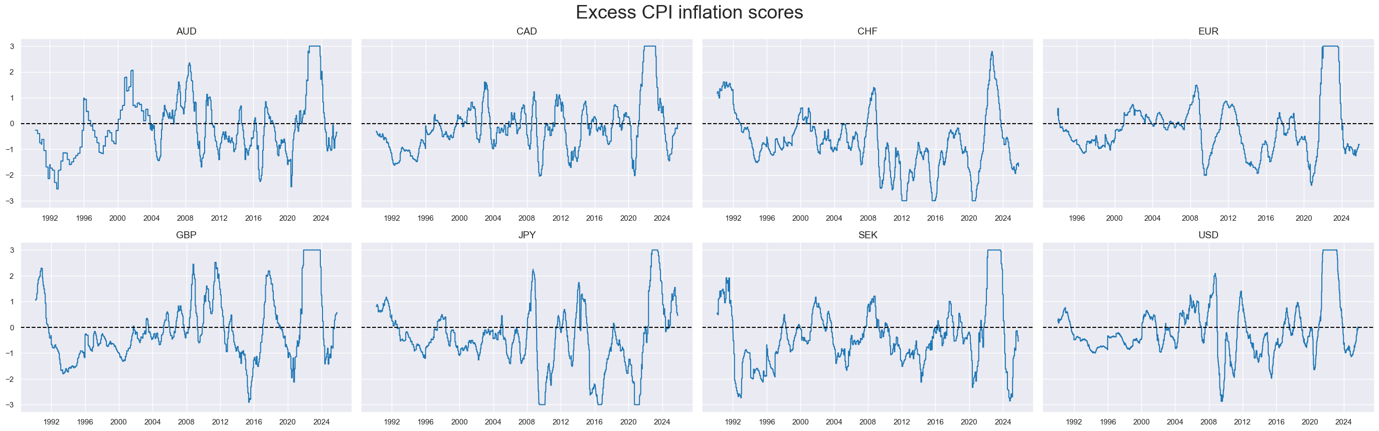
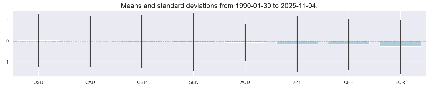
xcatx = ["XINFL_ZN"]
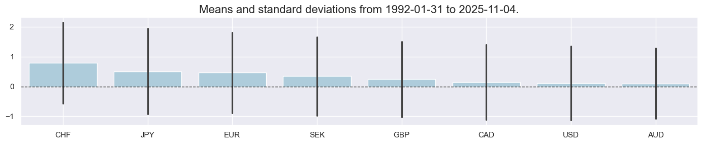
cidx = cids_ll
sdate = "1990-01-01"
msp.view_ranges(
dfx,
xcats=xcatx,
cids=cidx,
kind="bar",
sort_cids_by="mean",
size=(14, 3),
start=sdate,
)
msp.view_timelines(
dfx,
xcats=xcatx,
cids=cidx,
ncol=4,
cumsum=False,
start=sdate,
same_y=True,
all_xticks=True,
legend_fontsize=17,
title="Excess CPI inflation scores",
title_fontsize=27,
)
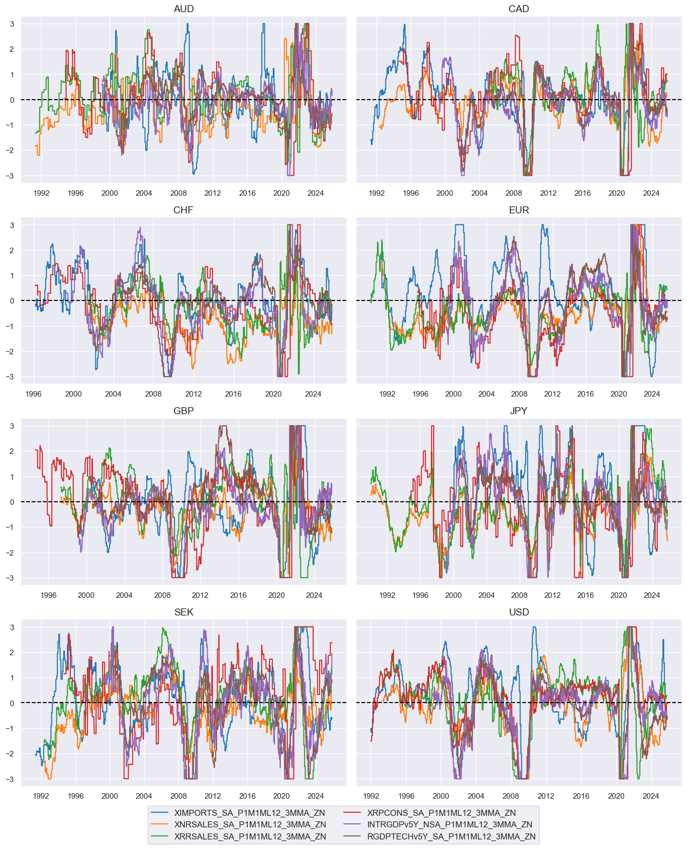
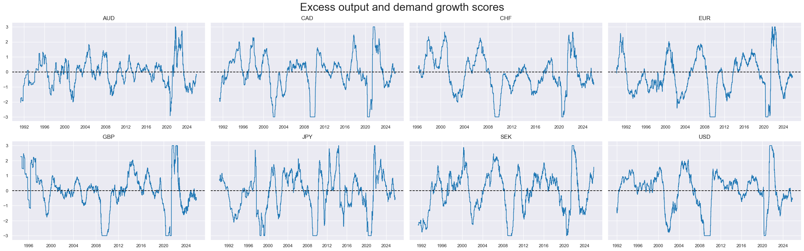
Excess growth and demand #
# Un-scored indicators and score weights

dict_xgrowth = {
    "XIMPORTS_SA_P1M1ML12_3MMA": 0.5,
    "XNRSALES_SA_P1M1ML12_3MMA": 0.5,
    "XRRSALES_SA_P1M1ML12_3MMA": 0.5,
    "XRPCONS_SA_P1M1ML12_3MMA": 0.5,
    "INTRGDPv5Y_NSA_P1M1ML12_3MMA": 1,
    "RGDPTECHv5Y_SA_P1M1ML12_3MMA": 1
}
# Excess growth

xcatx_nominal = [
    "IMPORTS_SA_P1M1ML12_3MMA",
    "NRSALES_SA_P1M1ML12_3MMA",
]
xcatx_real = ["RRSALES_SA_P1M1ML12_3MMA", "RPCONS_SA_P1M1ML12_3MMA"]

calcs = [f"X{xc} = {xc} - RGDP_SA_P1Q1QL4_20QMM - INFTEFF_BX" for xc in xcatx_nominal]
calcs += [f"X{xc} = {xc} - RGDP_SA_P1Q1QL4_20QMM" for xc in xcatx_real]

dfa = msp.panel_calculator(
    dfx,
    calcs=calcs,
    cids=cids,
)
dfx = msm.update_df(dfx, dfa)
# Normalization of excess growth indicators

cidx = cids_ll
xcatx = list(dict_xgrowth.keys())
sdate = "1990-01-01"

for xc in xcatx:
    dfaa = msp.make_zn_scores(
        dfx,
        xcat=xc,
        cids=cidx,
        sequential=True,
        min_obs=261 * 3,
        neutral="zero",
        pan_weight=1,  # variance estimated based on panel and cross-sectional variation
        thresh=3,
        postfix="_ZN",
        est_freq="m",
    )
    dfa = msm.update_df(dfa, dfaa)

dfx = msm.update_df(dfx, dfa)
xgrowthz = [k + "_ZN" for k in list(dict_xgrowth.keys())]
cidx = cids_ll
xcatx = xgrowthz

msp.view_timelines(
    dfx,
    xcats=xcatx,
    cids=cidx,
    ncol=2,
    start="1990-01-01",
    same_y=True,
    all_xticks=True,
)
# Weighted linear combination

cidx = cids_ll
xcatx = xgrowthz
weights = list(dict_xgrowth.values())
czs = "XGROWTH"

dfa = msp.linear_composite(
    dfx,
    xcats=xcatx,
    cids=cidx,
    weights=weights,
    normalize_weights=True,
    complete_xcats=False,  # score works with what is available
    new_xcat=czs,
)
dfx = msm.update_df(dfx, dfa)

# Re-scoring

dfa = msp.make_zn_scores(
    dfx,
    xcat=czs,
    cids=cidx,
    sequential=True,
    min_obs=261 * 5,
    neutral="zero",
    pan_weight=1,
    thresh=3,
    postfix="_ZN",
    est_freq="m",
)
dfx = msm.update_df(dfx, dfa)
xcatx = ["XGROWTH_ZN"]
cidx = cids_ll
sdate = "1990-01-01"

msp.view_ranges(
    df=dfx,
    xcats=xcatx,
    cids=cidx,
    kind="bar",
    sort_cids_by="mean",
    size=(14, 3),
    start=sdate,
)

msp.view_timelines(
    dfx,
    xcats=xcatx,
    cids=cidx,
    ncol=4,
    cumsum=False,
    start=sdate,
    same_y=True,
    all_xticks=True,
    legend_fontsize=17,
    title="Excess output and demand growth scores",
    title_fontsize=27,
)
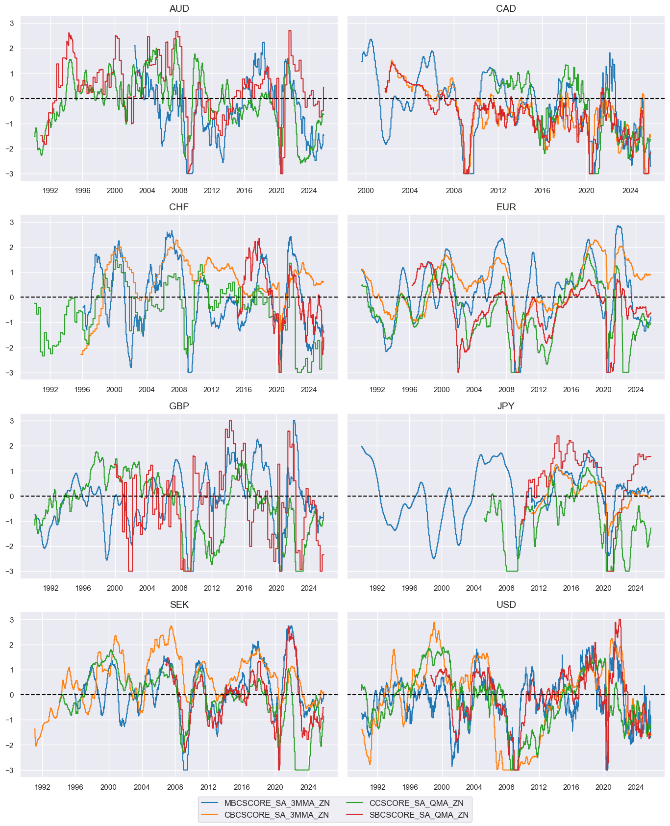
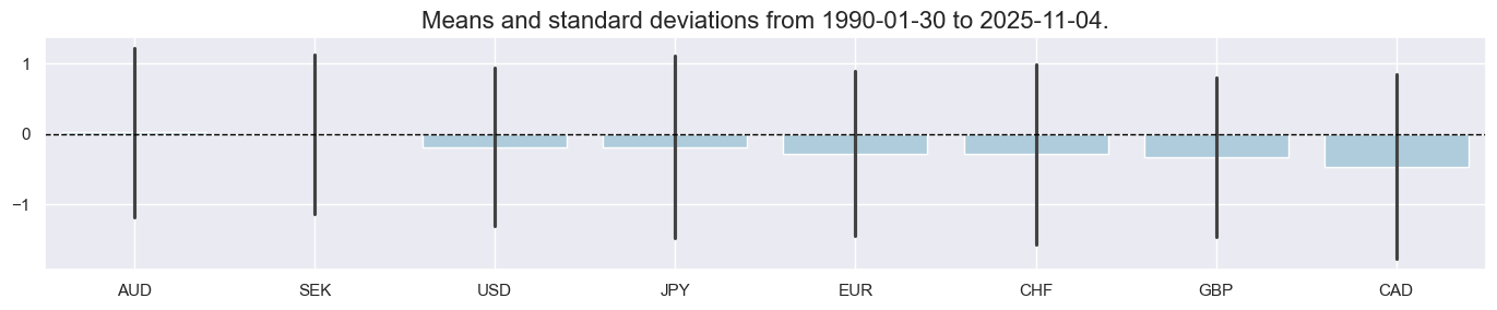
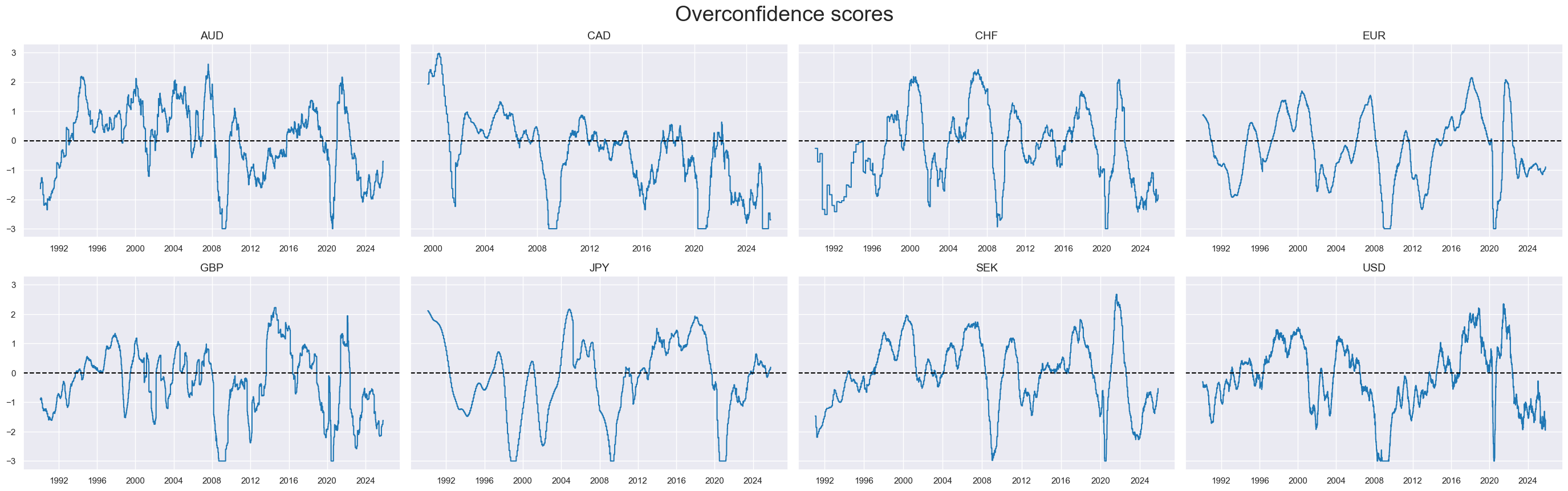
Overconfidence #
dict_xconf = {
    "MBCSCORE_SA_3MMA": 1,
    "CBCSCORE_SA_3MMA": 0.2,  # construction is small
    "CCSCORE_SA_QMA": 1,
    "SBCSCORE_SA_QMA": 1,
}
# Normalization of excess growth indicators

cidx = cids_ll
xcatx = list(dict_xconf.keys())
sdate = "1990-01-01"

for xc in xcatx:
    dfaa = msp.make_zn_scores(
        dfx,
        xcat=xc,
        cids=cidx,
        sequential=True,
        min_obs=261 * 3,
        neutral="zero",
        pan_weight=1,  # variance estimated based on panel and cross-sectional variation
        thresh=3,
        postfix="_ZN",
        est_freq="m",
    )
    dfa = msm.update_df(dfa, dfaa)

dfx = msm.update_df(dfx, dfa)
xconfz = [k + "_ZN" for k in list(dict_xconf.keys())]
cidx = cids_ll
xcatx = xconfz

msp.view_timelines(
    dfx,
    xcats=xcatx,
    cids=cidx,
    ncol=2,
    start="1990-01-01",
    same_y=True,
    all_xticks=True,
)
# Weighted linear combination

cidx = cids_ll
xcatx = xconfz
weights = list(dict_xconf.values())
czs = "XCONF"

dfa = msp.linear_composite(
    dfx,
    xcats=xcatx,
    cids=cidx,
    weights=weights,
    normalize_weights=True,
    complete_xcats=False,  # score works with what is available
    new_xcat=czs,
)
dfx = msm.update_df(dfx, dfa)

# Re-scoring

dfa = msp.make_zn_scores(
    dfx,
    xcat=czs,
    cids=cidx,
    sequential=True,
    min_obs=261 * 5,
    neutral="zero",
    pan_weight=1,
    thresh=3,
    postfix="_ZN",
    est_freq="m",
)
dfx = msm.update_df(dfx, dfa)
xcatx = ["XCONF_ZN"]
cidx = cids_ll
sdate = "1990-01-01"

msp.view_ranges(
    dfx,
    xcats=xcatx,
    cids=cidx,
    kind="bar",
    sort_cids_by="mean",
    size=(14, 3),
    start=sdate,
)

msp.view_timelines(
    dfx,
    xcats=xcatx,
    cids=cidx,
    ncol=4,
    cumsum=False,
    start=sdate,
    same_y=True,
    all_xticks=True,
    legend_fontsize=17,
    title="Overconfidence scores",
    title_fontsize=27,
)
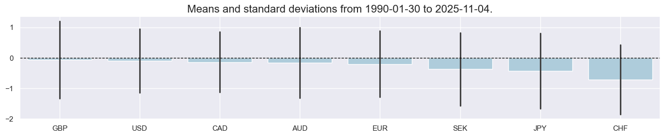
Composite factor scores #
# Turn factors negative (convention)

facts = ['XGROWTH_ZN', 'XINFL_ZN', 'XCONF_ZN']
calcs = [f"{fact}_NEG = -1 * {fact}" for fact in facts]
cidx = cids_ll

dfa = msp.panel_calculator(
    dfx,
    calcs=calcs,
    cids=cidx,
)
dfx = msm.update_df(dfx, dfa)
dict_facts = {
    "XINFL_ZN_NEG": 0.5,
    "XGROWTH_ZN_NEG": 0.4,
    "XCONF_ZN_NEG": 0.1,
}

factz = [k for k in list(dict_facts.keys())]
# Weighted linear combinations with appropriate signs

dict_combs = {
    "SLACK": [factz, cids_ll, "1992-01-01"],
}

for k, v in dict_combs.items():
    xcatx, cidx, sdate = v
    weights = [dict_facts[k] for k in xcatx]
    czs = k

    dfa = msp.linear_composite(
        dfx,
        xcats=xcatx,
        cids=cidx,
        weights=weights,
        normalize_weights=True,
        complete_xcats=False,  # score works with what is available
        new_xcat=czs,
        start=sdate,
    )
    dfx = msm.update_df(dfx, dfa)

    # Re-scoring

    dfa = msp.make_zn_scores(
        dfx,
        xcat=czs,
        cids=cidx,
        sequential=True,
        min_obs=261 * 5,
        neutral="zero",
        pan_weight=1,
        thresh=3,
        postfix="_ZN",
        est_freq="m",
    )
    dfx = msm.update_df(dfx, dfa)

combz = [k + "_ZN" for k in dict_combs.keys()]
xcatx = combz
cidx = cids_ll
sdate = "1990-01-01"
msp.view_ranges(
dfx,
xcats=xcatx,
cids=cidx,
kind="bar",
sort_cids_by="mean",
size=(14, 3),
start=sdate,
)
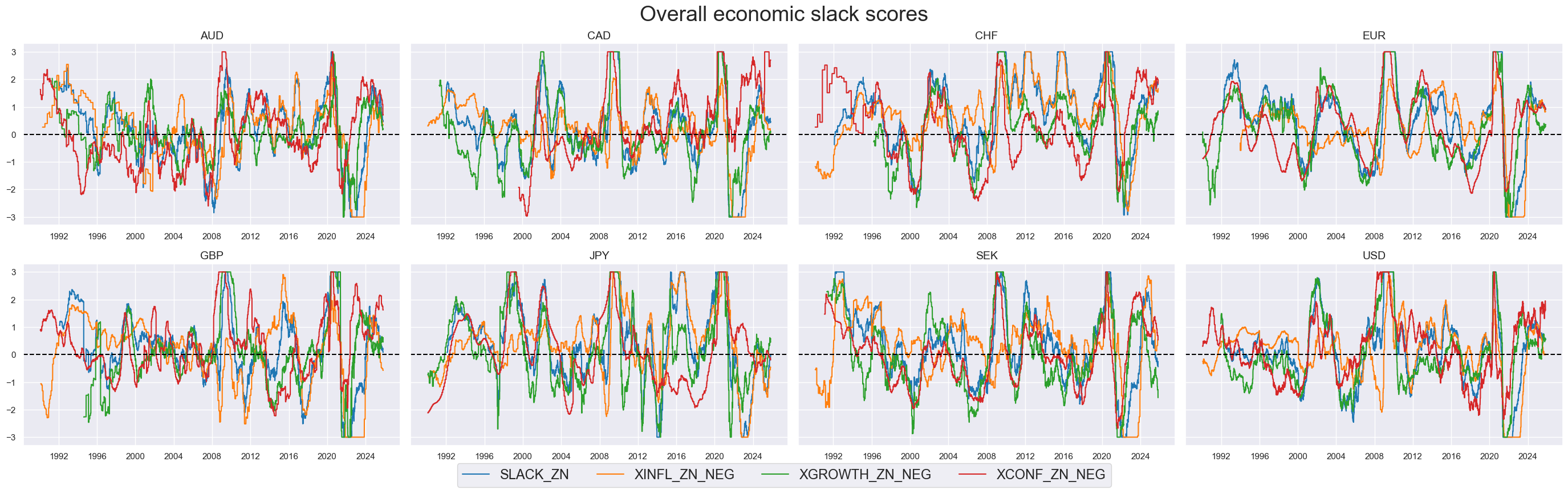
msp.view_timelines(
dfx,
xcats=xcatx + factz,
cids=cidx,
ncol=4,
cumsum=False,
start=sdate,
same_y=True,
all_xticks=True,
legend_fontsize=17,
title="Overall economic slack scores",
title_fontsize=27,
)
Target returns #
# Risk-parity equity-duration return

calc_edc = [
    "EQDUXR_RP = EQXR_VT10 + DU05YXR_VT10",
]
dfa = msp.panel_calculator(dfx, calcs=calc_edc, cids=cids)
dfx = msm.update_df(dfx, dfa)
# Vol estimation of risk parity positions

dfa = msp.historic_vol(
    dfx, xcat="EQDUXR_RP", cids=cids, lback_meth="xma", postfix="_ASD"
)
dfx = msm.update_df(dfx, dfa)

dft = dfa.pivot(index="real_date", columns="cid", values="value")
dftx = dft.resample("BM").last().reindex(dft.index).ffill().shift(1)
dfax = dftx.unstack().reset_index().rename({0: "value"}, axis=1)
dfax["xcat"] = "EQDUXR_RP_ASDML1"
dfx = msm.update_df(dfx, dfax)

# Vol-target risk parity performance indicators

calc_vaj = [
    "EQDUXR_RPVT10 = 10 * EQDUXR_RP / EQDUXR_RP_ASDML1",
]
dfa = msp.panel_calculator(dfx, calcs=calc_vaj, cids=cids)
dfx = msm.update_df(dfx, dfa)
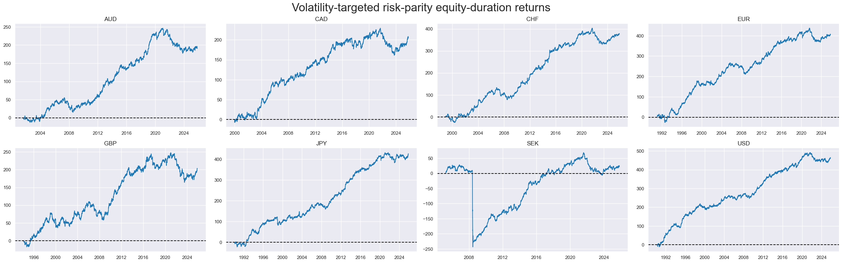
xcatx = ["EQDUXR_RPVT10"]
cidx = cids_ll
sdate = "1990-01-01"

msp.view_ranges(
    dfx,
    xcats=xcatx,
    cids=cidx,
    kind="box",
    sort_cids_by="mean",
    size=(14, 5),
    start=sdate,
)

msp.view_timelines(
    dfx,
    xcats=xcatx,
    cids=cidx,
    ncol=4,
    cumsum=True,
    start=sdate,
    same_y=False,
    all_xticks=True,
    legend_fontsize=17,
    title="Volatility-targeted risk-parity equity-duration returns",
    title_fontsize=27,
)

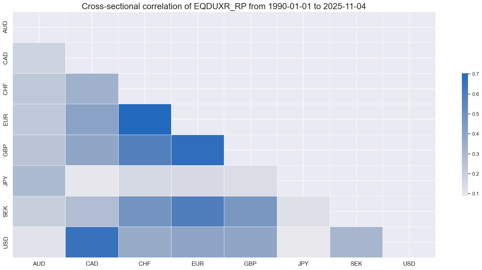
msp.correl_matrix(
    dfx,
    xcats=["EQDUXR_RP"],
    start = "1990-01-01",
    size = (18, 9),
)
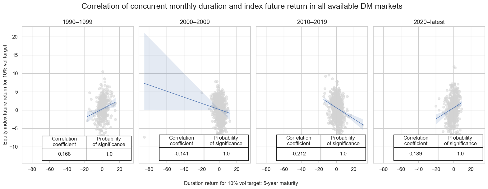
cr = {}

xcatx = ["DU05YXR_VT10", "EQXR_VT10"]
cidx = cids_ll

# Define periods and related parameters
periods = [
    ("1990-01-01", "2000-01-01"),
    ("2000-01-01", "2010-01-01"),
    ("2010-01-01", "2020-01-01"),
    ("2020-01-01", None)


]

# Initialize container for CategoryRelations
cat_rels = []

# Loop through periods to create CategoryRelations
for start_date, end_date in periods:
    cr = msp.CategoryRelations(
        dfx,
        xcats=xcatx,
        cids=cidx,
        freq="M",
        lag=0,
        xcat_aggs=["sum", "sum"],
        start=start_date,
        end=end_date,
        # xcat_trims=[8, 8],  # Optional: Trimming if needed
    )
    cat_rels.append(cr)

# Plot using multiple_reg_scatter
msv.multiple_reg_scatter(
    cat_rels=cat_rels,
    ncol=4,
    nrow=1,
    figsize=(16, 6),
    title="Correlation of concurrent monthly duration and index future return in all available DM markets",
    title_fontsize=18,
    xlab="Duration return for 10% vol target: 5-year maturity ",
    ylab="Equity index future return for 10% vol target",
    coef_box="lower right",
    prob_est="pool",
    coef_box_size=(0.8, 2.5),
    single_chart=True,
    subplot_titles=["1990–1999", "2000–2009", "2010–2019", "2020–latest" ],
)
Value checks #
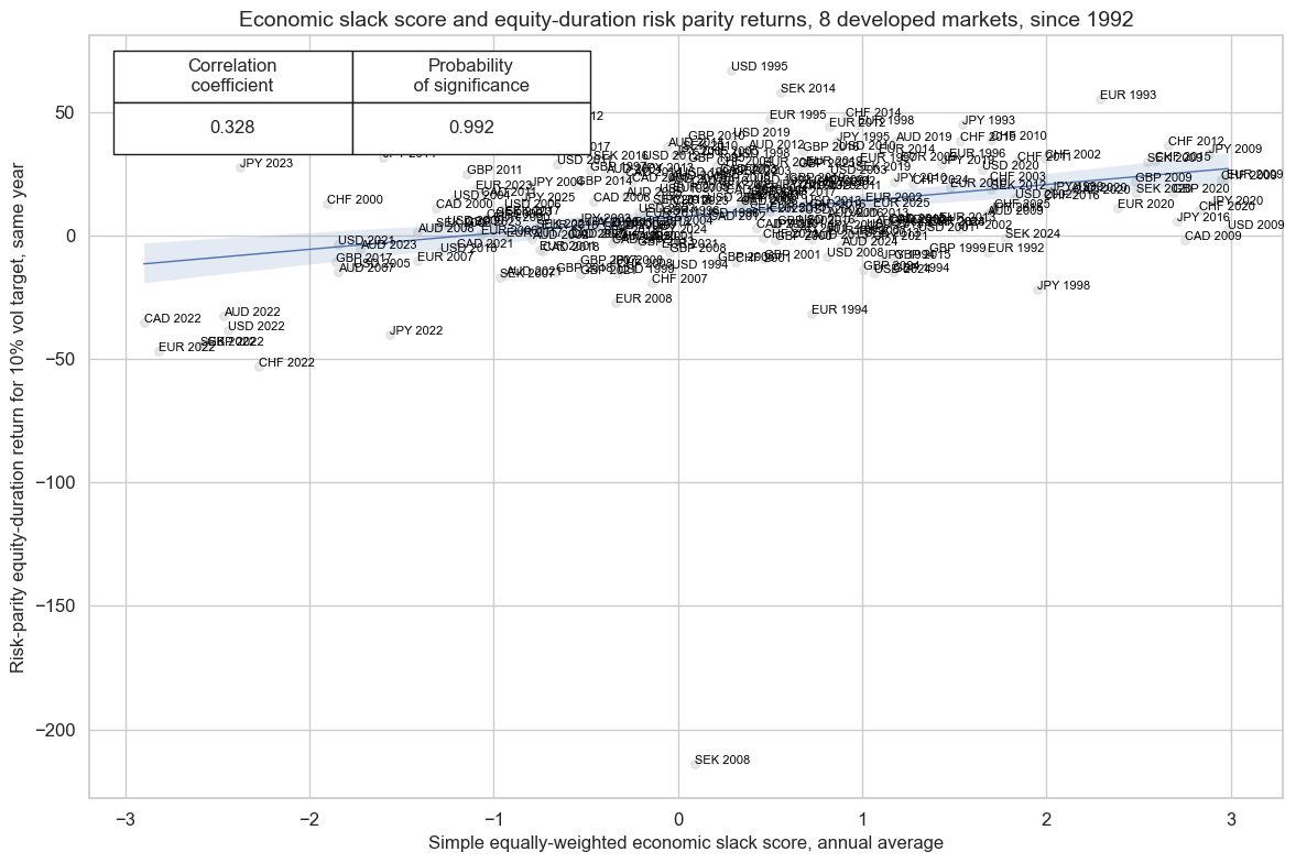
Basic empirics #
# Define all potential features for further analysis

xcatx = combz + ["EQDUXR_RP", "EQDUXR_RPVT10"]

msm.check_availability(dfx, xcats=xcatx, missing_recent=False)
feats = {"SLACK_ZN": "Simple equally-weighted economic slack score, annual average"}
target = {"EQDUXR_RPVT10": "Risk-parity equity-duration position, % local-currency return"}
cidx=cids_ll

cr_long = msp.CategoryRelations(
    dfx,
    xcats=[list(feats.keys())[0], list(target.keys())[0]],
    cids=cidx,
    freq="A",
    lag=0,
    xcat_aggs=["mean", "sum"],
    start="1990-01-01",
    xcat_trims=[None, None],
)
cr_long.reg_scatter(
    labels=True,
    coef_box = "upper left",
    prob_est = "map",
    title="Economic slack score and equity-duration risk parity returns, 8 developed markets, since 1992",
    xlab="Simple equally-weighted economic slack score, annual average",
    ylab="Risk-parity equity-duration return for 10% vol target, same year",
)
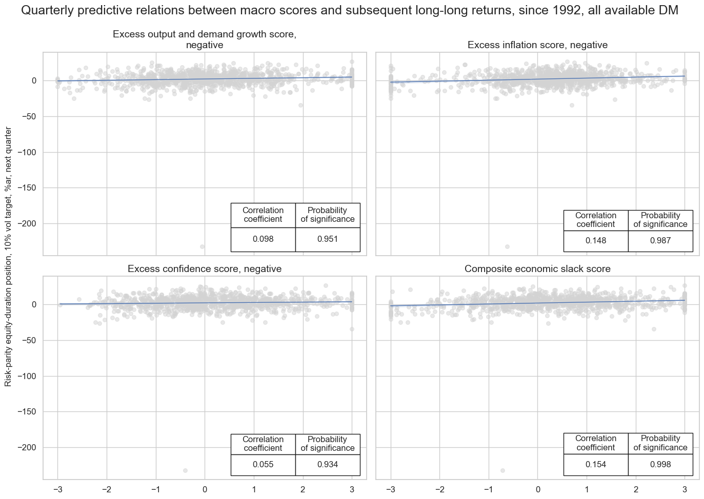
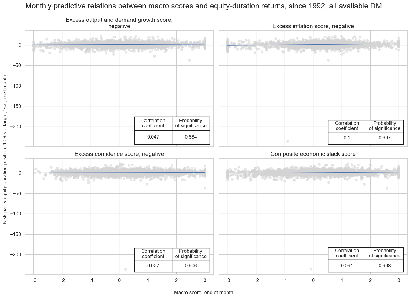
feats = {
    "XGROWTH_ZN_NEG": "Excess output and demand growth score, negative",
    "XINFL_ZN_NEG": "Excess inflation score, negative",
    "XCONF_ZN_NEG": "Excess confidence score, negative",
    "SLACK_ZN": "Composite economic slack score",
}

target = {"EQDUXR_RPVT10": "Risk-parity equity-duration position, % local-currency return"}
cidx = cids_ll

cr = {}

for sig in list(feats.keys()):
    cr[sig] = msp.CategoryRelations(
        dfx,
        xcats=[sig, list(target.keys())[0]],
        cids=cidx,
        freq="Q",
        lag=1,
        xcat_aggs=["last", "sum"],
        start="1990-01-01",
    )

msv.multiple_reg_scatter(
    cat_rels=[v for k, v in cr.items()],
    ncol=2,
    nrow=2,
    figsize=(14, 10),
    title="Quarterly predictive relations between macro scores and subsequent long-long returns, since 1992, all available DM",
    title_fontsize=18,
    xlab=None,
    ylab="Risk-parity equity-duration position, 10% vol target, %ar, next quarter",
    coef_box="lower right",
    prob_est="map",
    single_chart=True,
    subplot_titles=[feats[key] for key in feats.keys()],
)
Slack-based DM strategies from 1992 #
Specs and panel test #
dict_slack = {
    "sigs": list(feats.keys()),
    "labs": list(feats.values()),
    "targ": "EQDUXR_RPVT10",
    "cidx": cids_ll,
    "start": "1992-01-01",
    "crs": None,
    "srr": None,
    "pnls": None,
}
dix = dict_slack

sigs = dix["sigs"]
targ = dix["targ"]
cidx = dix["cidx"]
start = dix["start"]

# Initialize the dictionary to store CategoryRelations instances

dict_cr = {}

for sig in sigs:
    lab = sig + "_" + targ
    dict_cr[lab] = msp.CategoryRelations(
        dfx,
        xcats=[sig, targ],
        cids=cidx,
        freq="M",
        lag=1,
        xcat_aggs=["last", "sum"],
        start=start,
    )

dix["crs"] = dict_cr
# Plotting panel scatters

dix = dict_slack
dict_cr = dix["crs"]
labs = dix["labs"]

crs = list(dict_cr.values())
crs_keys = list(dict_cr.keys())

msv.multiple_reg_scatter(
    cat_rels=crs,
    ncol=2,
    nrow=2,
    figsize=(14, 10),
    title="Monthly predictive relations between macro scores and equity-duration returns, since 1992, all available DM",
    title_fontsize=18,
    xlab="Macro score, end of month",
    ylab="Risk-parity equity-duration position, 10% vol target, %ar, next month",
    coef_box="lower right",
    prob_est="map",
    single_chart=True,
    subplot_titles=labs,
)
Accuracy and correlation check #
dix = dict_slack

sigs = dix["sigs"]
targ = dix["targ"]
cidx = dix["cidx"]
start = dix["start"]

srr = mss.SignalReturnRelations(
    dfx,
    cids=cidx,
    sigs=sigs,
    rets=targ,
    freqs="M",
    start=start,
)

display(srr.signals_table().sort_index().astype("float").round(3))

dix["srr"] = srr
| accuracy | bal_accuracy | pos_sigr | pos_retr | pos_prec | neg_prec | pearson | pearson_pval | kendall | kendall_pval | auc | ||||
|---|---|---|---|---|---|---|---|---|---|---|---|---|---|---|
| Return | Signal | Frequency | Aggregation | |||||||||||
| EQDUXR_RPVT10 | SLACK_ZN | M | last | 0.562 | 0.541 | 0.594 | 0.619 | 0.653 | 0.430 | 0.091 | 0.000 | 0.068 | 0.000 | 0.542 |
| XCONF_ZN_NEG | M | last | 0.526 | 0.518 | 0.534 | 0.619 | 0.636 | 0.400 | 0.027 | 0.152 | 0.028 | 0.027 | 0.519 | |
| XGROWTH_ZN_NEG | M | last | 0.514 | 0.513 | 0.507 | 0.620 | 0.632 | 0.393 | 0.047 | 0.013 | 0.038 | 0.003 | 0.514 | |
| XINFL_ZN_NEG | M | last | 0.577 | 0.543 | 0.663 | 0.619 | 0.648 | 0.438 | 0.100 | 0.000 | 0.068 | 0.000 | 0.541 |
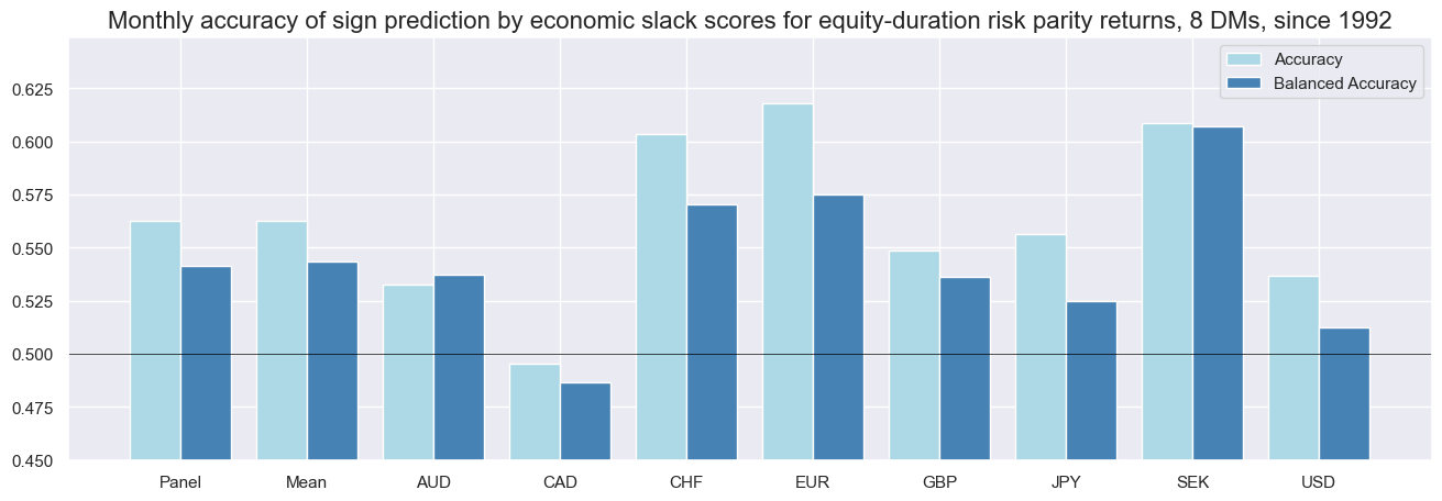
srr = dix["srr"]

srr.accuracy_bars(
    type="cross_section",
    sigs='SLACK_ZN',
    title="Monthly accuracy of sign prediction by economic slack scores for equity-duration risk parity returns, 8 DMs, since 1992",
    size=(16, 5),
)
Naive PnL #
# Simulate naive PnL

dix = dict_slack

sig = list(feats.keys())
targ = dix["targ"]
cidx = dix["cidx"]
start = dix["start"]

naive_pnl = msn.NaivePnL(
    dfx,
    ret=targ,
    sigs=sig,
    cids=cidx,
    start=start,
    bms=["USD_EQXR_NSA", "USD_DU05YXR_NSA"],
)

for bias in [0, 1]:
    for sig in list(feats.keys()):
        naive_pnl.make_pnl(
            sig,
            sig_add=bias,
            sig_op="zn_score_pan",
            thresh=2,
            leverage=1/8,
            rebal_freq="monthly",
            vol_scale=None,
            rebal_slip=1,
            pnl_name=sig + "_PZN" + str(bias),
        )

naive_pnl.make_long_pnl(label="Long only", vol_scale=None, leverage=1/8)
dix["pnls"] = naive_pnl
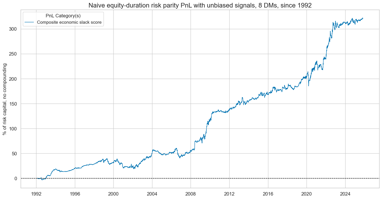
dix = dict_slack
sig = list(feats.keys())
cidx = dix["cidx"]
start = dix["start"]
naive_pnl = dix["pnls"]
pnls = [sig + "_PZN0" for sig in feats.keys()]
pnl_labels = {f"{list(feats.keys())[3]}_PZN0": list(feats.values())[3]}
naive_pnl.plot_pnls(
pnl_cats=[pnls[3]],
pnl_cids=["ALL"],
start=start,
title="Naive equity-duration risk parity PnL with unbiased signals, 8 DMs, since 1992",
title_fontsize=16,
figsize=(16, 8),
compounding=False,
xcat_labels=pnl_labels
)
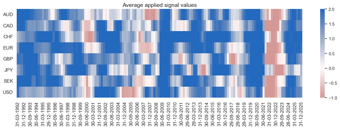
display(naive_pnl.evaluate_pnls(pnl_cats=pnls[3:]))
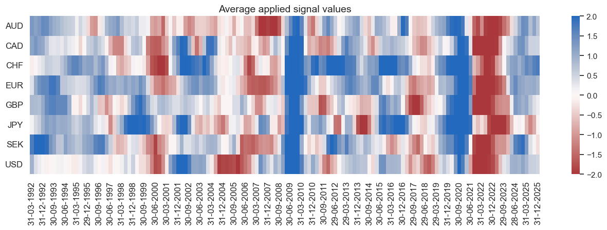
naive_pnl.signal_heatmap(pnls[3], freq="q", start=start, figsize=(16, 4))
| xcat | SLACK_ZN_PZN0 |
|---|---|
| Return % | 9.509743 |
| St. Dev. % | 10.2133 |
| Sharpe Ratio | 0.931114 |
| Sortino Ratio | 1.41053 |
| Max 21-Day Draw % | -28.408596 |
| Max 6-Month Draw % | -18.47332 |
| Peak to Trough Draw % | -29.057058 |
| Top 5% Monthly PnL Share | 0.712788 |
| USD_EQXR_NSA correl | 0.083847 |
| USD_DU05YXR_NSA correl | 0.045288 |
| Traded Months | 407 |
dix = dict_slack
sig = list(feats.keys())
cidx = dix["cidx"]
start = dix["start"]
naive_pnl = dix["pnls"]
pnls = [sig + "_PZN1" for sig in feats.keys()] + ["Long only"]
pnl_labels = {f"{list(feats.keys())[3]}_PZN1": list(feats.values())[3]}
pnl_labels["Long only"] = "Long only"
naive_pnl.plot_pnls(
pnl_cats=pnls[3:],
pnl_cids=["ALL"],
start=start,
title="Naive equity-duration risk parity PnL, 8 DMs, since 1992",
title_fontsize=16,
figsize=(16, 8),
compounding=False,
xcat_labels=pnl_labels
)
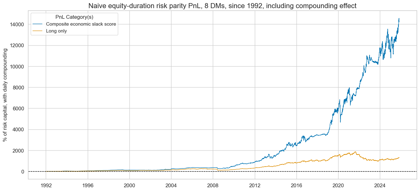
naive_pnl.plot_pnls(
pnl_cats=pnls[3:],
pnl_cids=["ALL"],
start=start,
title="Naive equity-duration risk parity PnL, 8 DMs, since 1992, including compounding effect",
title_fontsize=16,
figsize=(16, 7),
compounding=True,
xcat_labels=pnl_labels
)
display(naive_pnl.evaluate_pnls(pnl_cats=pnls[3:]))
naive_pnl.signal_heatmap(pnls[3], freq="q", start=start, figsize=(16, 4))
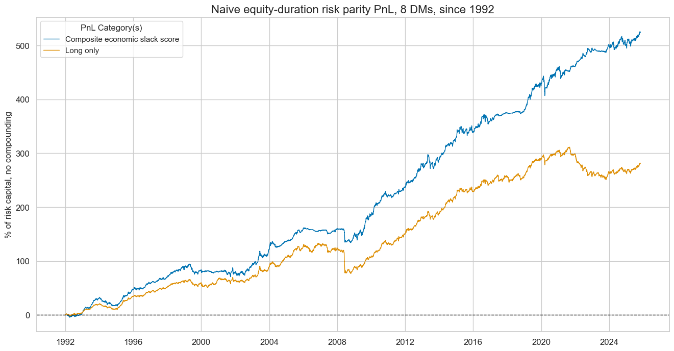
| xcat | SLACK_ZN_PZN1 | Long only |
|---|---|---|
| Return % | 15.508532 | 8.283334 |
| St. Dev. % | 12.601055 | 9.710594 |
| Sharpe Ratio | 1.230733 | 0.85302 |
| Sortino Ratio | 1.758124 | 1.146228 |
| Max 21-Day Draw % | -35.694971 | -41.620314 |
| Max 6-Month Draw % | -24.874558 | -45.695591 |
| Peak to Trough Draw % | -36.481491 | -60.13675 |
| Top 5% Monthly PnL Share | 0.428562 | 0.551973 |
| USD_EQXR_NSA correl | 0.277475 | 0.344707 |
| USD_DU05YXR_NSA correl | 0.253165 | 0.332896 |
| Traded Months | 407 | 407 |