FX trends and external balance headwinds #
This notebook serves as an illustration of the points discussed in the post “FX trend following and macro headwinds” available on the Macrosynergy website.
The post argues that macroeconomic data can provide valuable insights into the headwinds or tailwinds that may affect the continuation of market price trends. In the FX space, for example, the sustainability of a positive return trend in a currency is less likely if concurrent economic data suggest a deterioration in the competitiveness of the local economy. These macro indicators of setback risk may not be easily detected using traditional statistical methods for identifying return predictors, as their effects can compete with dominant trends and exhibit non-linear and concentrated patterns.
To address this issue, the post suggests adjusting standard global FX trend-following strategies to account for changes in external balances. Empirical evidence supports the idea that such adjustments can significantly enhance the performance of FX trend following. In particular, the post compares the predictive power and economic value of the standard trend and the external balance dynamics scores separately, concluding that both are complimentary. It then considers two types of trend adjustment:
-
modifying the original trend signal by multiplying it with a coefficient based on the external dynamics score
-
averaging the original trend and external balance dynamics z-score.
The post concludes, that external balance adjustment for FX trend following strategy provides considerable economic value. The effect is particularly pronounced for emerging economies.
This notebook provides the essential code required to replicate the analysis discussed in the post.
Imports #
This notebook primarily relies on the standard packages available in the Python data science stack. However, there is an additional package
macrosynergy
that is required for two purposes:
-
Downloading JPMaQS data: The
macrosynergypackage facilitates the retrieval of JPMaQS data, which is used in the notebook. -
For the analysis of quantamental data and value propositions: The
macrosynergypackage provides functionality for performing quick analyses of quantamental data and exploring value propositions.
For detailed information and a comprehensive understanding of the
macrosynergy
package and its functionalities, please refer to the
“Introduction to Macrosynergy package”
on the Macrosynergy Academy or visit the following link on
Kaggle
.
To install the latest version of the package please use the command pip install macrosynergy –upgrade
import numpy as np
import pandas as pd
import matplotlib.pyplot as plt
import seaborn as sns


import macrosynergy.management as msm
import macrosynergy.panel as msp
import macrosynergy.signal as mss
import macrosynergy.pnl as msn
from macrosynergy.download import JPMaQSDownload


from datetime import timedelta, date, datetime
from itertools import combinations
import warnings
import os

warnings.simplefilter("ignore")
The JPMaQS indicators we consider are downloaded using the J.P. Morgan Dataquery API interface within the
macrosynergy
package. This is done by specifying ticker strings, formed by appending an indicator category code
DB(JPMAQS,<cross_section>_<category>,<info>)
, where
value
giving the latest available values for the indicator
eop_lag
referring to days elapsed since the end of the observation period
mop_lag
referring to the number of days elapsed since the mean observation period
grade
denoting a grade of the observation, giving a metric of real-time information quality.
After instantiating the
JPMaQSDownload
class within the
macrosynergy.download
module, one can use the
download(tickers,start_date,metrics)
method to easily download the necessary data, where
tickers
is an array of ticker strings,
start_date
is the first collection date to be considered and
metrics
is an array comprising the times series information to be downloaded. For more information see
here
.
To ensure reproducibility, only samples between January 2000 (inclusive) and May 2023 (exclusive) are considered.
# General cross-sections lists

cids_g3 = ["EUR", "JPY", "USD"]  # DM large currency areas
cids_dmsc = ["AUD", "CAD", "CHF", "GBP", "NOK", "NZD", "SEK"]  # DM small currency areas
cids_latm = ["BRL", "COP", "CLP", "MXN", "PEN"]  # Latam
cids_emea = ["CZK", "HUF", "ILS", "PLN", "RON", "RUB", "TRY", "ZAR"]  # EMEA
cids_emas = ["IDR", "INR", "KRW", "MYR", "PHP", "SGD", "THB", "TWD"]  # EM Asia ex China

cids_dm = cids_g3 + cids_dmsc
cids_em = cids_latm + cids_emea + cids_emas
cids = cids_dm + cids_em

# FX cross-section lists

cids_nofx = ["EUR", "USD", "SGD", "RUB"]  # not suitable for analysis
cids_fx = list(set(cids) - set(cids_nofx))

cids_dmfx = list(set(cids_dm).intersection(cids_fx))
cids_emfx = list(set(cids_em).intersection(cids_fx))

cids_eur = ["CHF", "CZK", "HUF", "NOK", "PLN", "RON", "SEK"]  # trading against EUR
cids_eud = ["GBP", "TRY"]  # trading against EUR and USD
cids_usd = list(set(cids_fx) - set(cids_eur + cids_eud))  # trading against USD
# Category tickers

xbts = [  # long-term trends
    "BXBGDPRATIO_NSA_12MMAv60MMA",
    "BXBGDPRATIO_NSA_12MMAv120MMA",
    "MTBGDPRATIO_SA_3MMAv24MMA",
    "MTBGDPRATIO_SA_3MMAv60MMA",
    "MTBGDPRATIO_SA_3MMAv120MMA",
]

xbds = [  # shorter-term dynamcis
    "BXBGDPRATIO_NSA_12MMA_D1M1ML3",
    "MTBGDPRATIO_SA_3MMA_D1M1ML3",
    "MTBGDPRATIO_SA_6MMA_D1M1ML6",
    "MTBGDPRATIO_NSA_12MMA_D1M1ML3",
]

main = xbts + xbds

rets = [
    "FXXR_NSA",
    "FXXR_VT10",
    "FXXRHvGDRB_NSA",
    "EQXR_NSA",
    "FXTARGETED_NSA",
    "FXUNTRADABLE_NSA",
]

xcats = main + rets

# Resultant tickers

tickers = [cid + "_" + xcat for cid in cids for xcat in xcats]
print(f"Maximum number of tickers is {len(tickers)}")
Maximum number of tickers is 465
The description of each JPMaQS category is available under Macro quantamental academy , or JPMorgan Markets (password protected). For tickers used in this notebook see External ratios trends , FX forward returns , and Equity index future returns .
# Download series from J.P. Morgan DataQuery by tickers

start_date = "2000-01-01"
end_date = "2023-05-01"

# Retrieve credentials

client_id: str = os.getenv("DQ_CLIENT_ID")
client_secret: str = os.getenv("DQ_CLIENT_SECRET")

with JPMaQSDownload(client_id=client_id, client_secret=client_secret) as dq:
    df = dq.download(
        tickers=tickers,
        start_date=start_date,
        end_date=end_date,
        suppress_warning=True,
        metrics=["all"],
        report_time_taken=True,
        show_progress=True,
    )
Downloading data from JPMaQS.
Timestamp UTC:  2025-06-25 13:10:12
Connection successful!
Requesting data: 40%|████ | 47/117 [00:09<00:14, 4.97it/s]
Requesting data: 100%|██████████| 117/117 [00:26<00:00,  4.49it/s]
Downloading data: 100%|██████████| 117/117 [00:43<00:00,  2.67it/s]
Time taken to download data: 	76.02 seconds.
Some expressions are missing from the downloaded data. Check logger output for complete list.
85 out of 2325 expressions are missing. To download the catalogue of all available expressions and filter the unavailable expressions, set `get_catalogue=True` in the call to `JPMaQSDownload.download()`.
dfx = df.copy()
display(dfx["xcat"].unique())
display(dfx["cid"].unique())
dfx["ticker"] = dfx["cid"] + "_" + dfx["xcat"]
# dfx.head(3)
array(['BXBGDPRATIO_NSA_12MMA_D1M1ML3', 'BXBGDPRATIO_NSA_12MMAv120MMA',
       'BXBGDPRATIO_NSA_12MMAv60MMA', 'EQXR_NSA', 'FXUNTRADABLE_NSA',
       'FXXRHvGDRB_NSA', 'FXTARGETED_NSA', 'FXXR_NSA', 'FXXR_VT10',
       'MTBGDPRATIO_SA_3MMA_D1M1ML3', 'MTBGDPRATIO_SA_3MMAv120MMA',
       'MTBGDPRATIO_NSA_12MMA_D1M1ML3', 'MTBGDPRATIO_SA_3MMAv24MMA',
       'MTBGDPRATIO_SA_3MMAv60MMA', 'MTBGDPRATIO_SA_6MMA_D1M1ML6'],
      dtype=object)
array(['AUD', 'BRL', 'CAD', 'CHF', 'CLP', 'COP', 'CZK', 'EUR', 'GBP',
       'HUF', 'IDR', 'ILS', 'INR', 'JPY', 'KRW', 'MXN', 'MYR', 'NOK',
       'NZD', 'PEN', 'PHP', 'PLN', 'RON', 'RUB', 'SEK', 'SGD', 'THB',
       'TRY', 'TWD', 'USD', 'ZAR'], dtype=object)
scols = ["cid", "xcat", "real_date", "value"]  # required columns
dfx = df[scols].copy()
dfx.info()
<class 'pandas.core.frame.DataFrame'>
RangeIndex: 2620109 entries, 0 to 2620108
Data columns (total 4 columns):
 #   Column     Dtype
---  ------     -----
 0   cid        object
 1   xcat       object
 2   real_date  datetime64[ns]
 3   value      float64
dtypes: datetime64[ns](1), float64(1), object(2)
memory usage: 80.0+ MB
Blacklist dictionaries #
Identifying and isolating periods of official exchange rate targets, illiquidity, or convertibility-related distortions in FX markets is the first step in creating an FX trading strategy. These periods can significantly impact the behavior and dynamics of currency markets, and failing to account for them can lead to inaccurate or misleading findings.
dfb = df[df["xcat"].isin(["FXTARGETED_NSA", "FXUNTRADABLE_NSA"])].loc[
    :, ["cid", "xcat", "real_date", "value"]
]
dfba = (
    dfb.groupby(["cid", "real_date"])
    .aggregate(value=pd.NamedAgg(column="value", aggfunc="max"))
    .reset_index()
)
dfba["xcat"] = "FXBLACK"
fxblack = msp.make_blacklist(dfba, "FXBLACK")
fxblack
{'BRL': (Timestamp('2012-12-03 00:00:00'), Timestamp('2013-09-30 00:00:00')),
 'CHF': (Timestamp('2011-10-03 00:00:00'), Timestamp('2015-01-30 00:00:00')),
 'CZK': (Timestamp('2014-01-01 00:00:00'), Timestamp('2017-07-31 00:00:00')),
 'ILS': (Timestamp('2000-01-03 00:00:00'), Timestamp('2005-12-30 00:00:00')),
 'INR': (Timestamp('2000-01-03 00:00:00'), Timestamp('2004-12-31 00:00:00')),
 'MYR_1': (Timestamp('2000-01-03 00:00:00'), Timestamp('2007-11-30 00:00:00')),
 'MYR_2': (Timestamp('2018-07-02 00:00:00'), Timestamp('2023-05-01 00:00:00')),
 'PEN': (Timestamp('2021-07-01 00:00:00'), Timestamp('2021-07-30 00:00:00')),
 'RON': (Timestamp('2000-01-03 00:00:00'), Timestamp('2005-11-30 00:00:00')),
 'RUB_1': (Timestamp('2000-01-03 00:00:00'), Timestamp('2005-11-30 00:00:00')),
 'RUB_2': (Timestamp('2022-02-01 00:00:00'), Timestamp('2023-05-01 00:00:00')),
 'SGD': (Timestamp('2000-01-03 00:00:00'), Timestamp('2023-05-01 00:00:00')),
 'THB': (Timestamp('2007-01-01 00:00:00'), Timestamp('2008-11-28 00:00:00')),
 'TRY_1': (Timestamp('2000-01-03 00:00:00'), Timestamp('2003-09-30 00:00:00')),
 'TRY_2': (Timestamp('2020-01-01 00:00:00'), Timestamp('2023-05-01 00:00:00'))}
Availability #
It is important to assess data availability before conducting any analysis. It allows identifying any potential gaps or limitations in the dataset, which can impact the validity and reliability of analysis and ensure that a sufficient number of observations for each selected category and cross-section is available as well as determining the appropriate time periods for analysis.
msm.check_availability(df, xcats=main, cids=cids)


Transformations and checks #
Features #
Long-term external ratios trends #
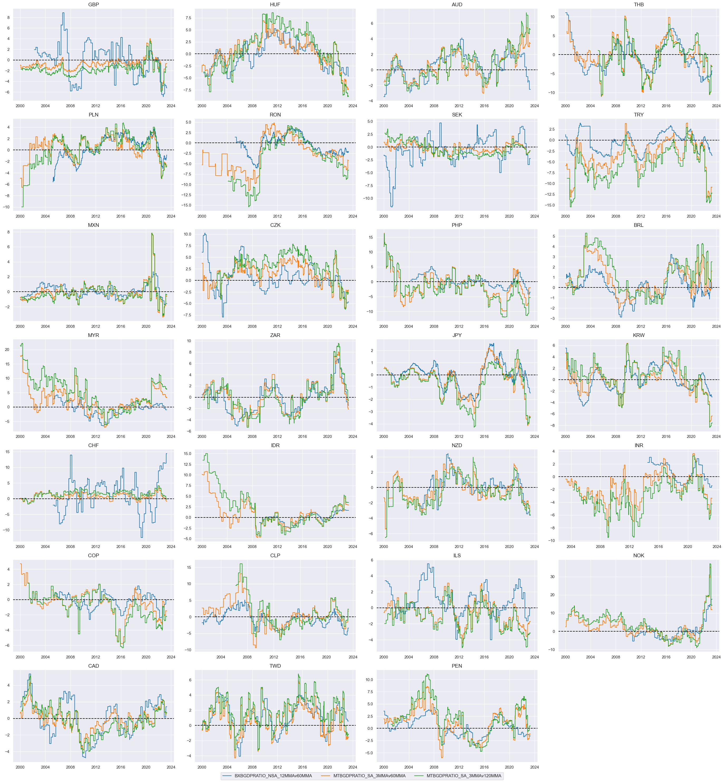
We start with collecting and displaying longer-term basic external balances trends on a timeline:
xcatx = [
    "BXBGDPRATIO_NSA_12MMAv60MMA",  # Basic external balance (current account plus net FDI trend), as % of GDP: 1-year average versus 5-year average
    "MTBGDPRATIO_SA_3MMAv60MMA",  # Merchandise trade balance, seasonally adjusted, as % of nominal GDP latest 3 months versus 5-year average
    "MTBGDPRATIO_SA_3MMAv120MMA",  # Merchandise trade balance, seasonally adjusted, as % of nominal GDP latest 3 months versus 10-year average
]
cidx = cids_fx

msp.view_timelines(
    dfx,
    xcats=xcatx,
    cids=cidx,
    ncol=4,
    cumsum=False,
    start="2000-01-01",
    same_y=False,
    size=(12, 12),
    all_xticks=True,
  )
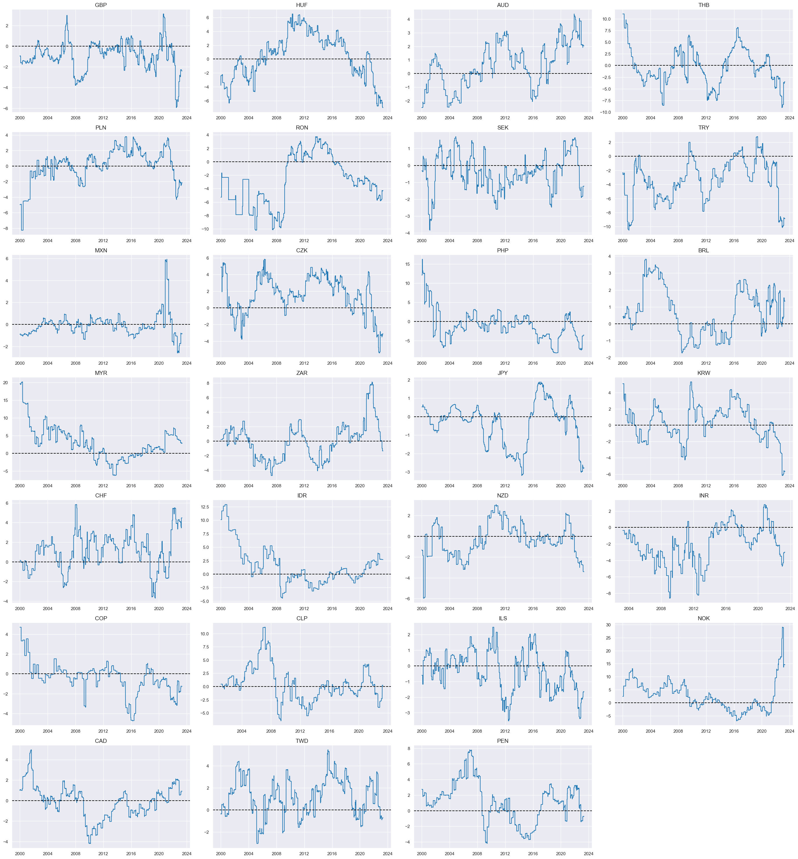
Next, we combine to simple trend averages with equal weights for all constituents and create the new trend indicator
XBTREND_AVG
:
dix = {
    "BXBGDPRATIO_NSA_12MMAv60MMA": 1 / 3,
    "MTBGDPRATIO_SA_3MMAv60MMA": 1 / 3,
    "MTBGDPRATIO_SA_3MMAv120MMA": 1 / 3,
}
cidx = cids_fx

dfa = msp.linear_composite(
    dfx,
    xcats=list(dix.keys()),
    weights=list(dix.values()),
    cids=cidx,
    complete_xcats=False,
    new_xcat="XBTREND_AVG",
)
dfx = msm.update_df(dfx, dfa)

xcatx = ["XBTREND_AVG"]

msp.view_timelines(
    dfx,
    xcats=xcatx,
    cids=cidx,
    ncol=4,
    cumsum=False,
    start="2000-01-01",
    same_y=False,
    size=(12, 12),
    all_xticks=True,
   )
Short-term external ratio changes #
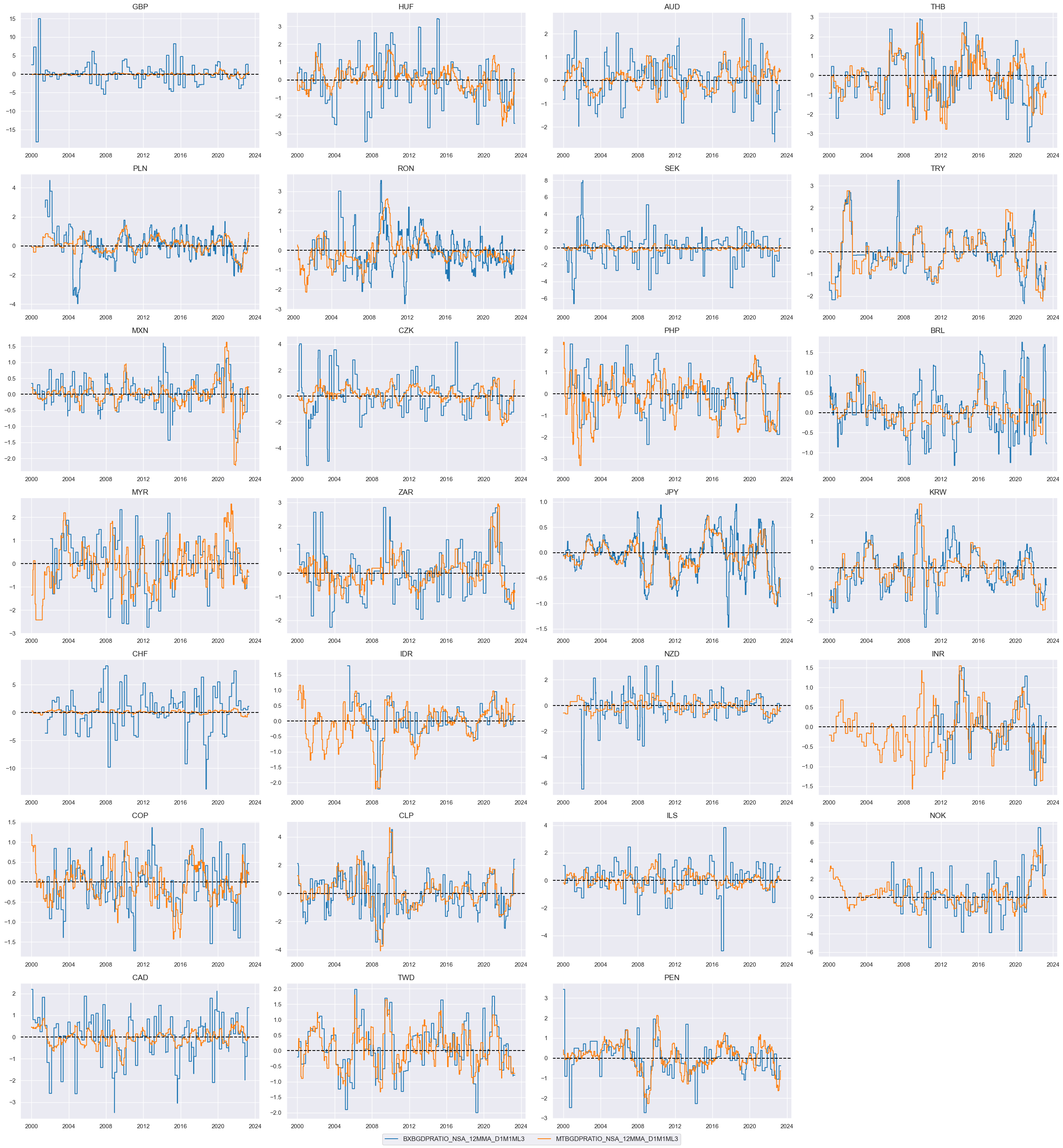
Separately we collect medium-term trade balance trends and basic external balance trends , and also display them on a timeline:
xcatx = [
    "BXBGDPRATIO_NSA_12MMA_D1M1ML3",  # Basic external balance as % of nominal GDP, 1-year moving average. change over the last three reported months.
    "MTBGDPRATIO_NSA_12MMA_D1M1ML3",
]  # Merchandise trade balance as % of nominal GDP, 1-year moving average, change over last three reported months.
cidx = cids_fx

msp.view_timelines(
    dfx,
    xcats=xcatx,
    cids=cidx,
    ncol=4,
    cumsum=False,
    start="2000-01-01",
    same_y=False,
    size=(12, 12),
    all_xticks=True,

)
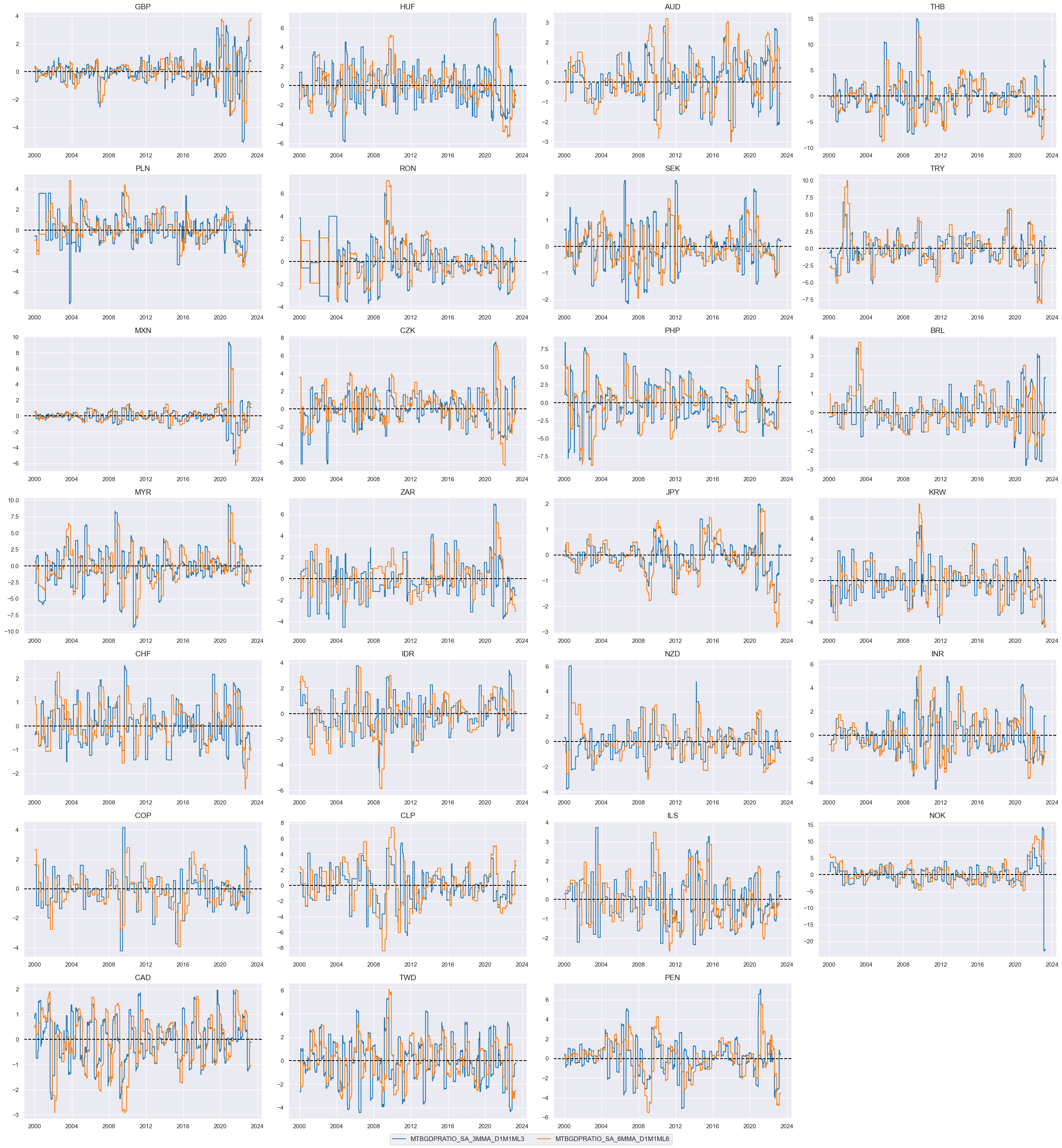
Here we collect two short-term trade balance trends : 3m/3m and 6m/6m and display them on a timeline:
xcatx = [
    "MTBGDPRATIO_SA_3MMA_D1M1ML3",  # Merchandise trade balance as % of nominal GDP, 3-month moving average over previous 3 months.
    "MTBGDPRATIO_SA_6MMA_D1M1ML6",  # Merchandise trade balance as % of nominal GDP, 6-month moving average over previous 6 months.
]
cidx = cids_fx

msp.view_timelines(
    dfx,
    xcats=xcatx,
    cids=cidx,
    ncol=4,
    cumsum=False,
    start="2000-01-01",
    same_y=False,
    size=(12, 12),
    all_xticks=True,
    title_adj=0.95,
    label_adj=0.05,
)
To standardize the variables for later comparisons and aggregations, we normalize them (create z-scores) and then average the indicators, giving effectively equal weights to all constituents (except for the two short-term trade balance changes, which are highly correlated and count as one):
xcatx = xbds  # shorter term dynamics
cidx = cids_fx

dfa = pd.DataFrame(columns=dfx.columns)
for xc in xcatx:
    dfaa = msp.make_zn_scores(
        dfx,
        xcat=xc,
        cids=cidx,
        sequential=True,
        min_obs=522,  # oos scaling after 2 years of panel data
        est_freq="m",
        neutral="zero",
        pan_weight=1,
        thresh=3,
        postfix="_ZN",
    )
    dfa = msm.update_df(dfa, dfaa)
dfx = msm.update_df(dfx, dfa)
dix = {
    "BXBGDPRATIO_NSA_12MMA_D1M1ML3_ZN": 1 / 3,
    "MTBGDPRATIO_NSA_12MMA_D1M1ML3_ZN": 1 / 3,
    "MTBGDPRATIO_SA_3MMA_D1M1ML3_ZN": 1 / 6,
    "MTBGDPRATIO_SA_6MMA_D1M1ML6_ZN": 1 / 6,
}
cidx = cids_fx

dfa = msp.linear_composite(
    dfx,
    xcats=list(dix.keys()),
    weights=list(dix.values()),
    cids=cidx,
    complete_xcats=False,
    new_xcat="XBDYNZ_AVG",
)
dfx = msm.update_df(dfx, dfa)
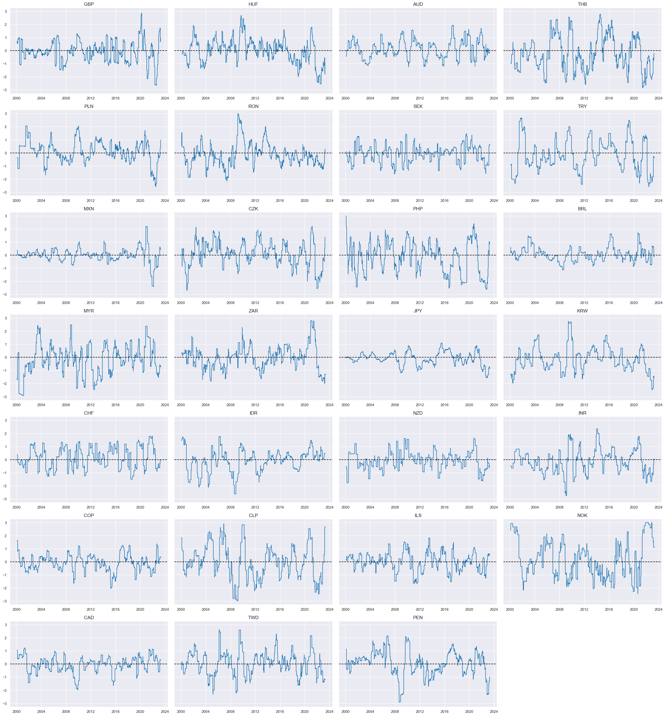
Here we display the newly created composite measure of shorter-term dynamics indicator
XBDYNZ_AVG
on a timeline. The letter
Z
in the name indicates that it is normalized around zero:
xcatx = [
    "XBDYNZ_AVG",
]
cidx = cids_fx

msp.view_timelines(
    dfx,
    xcats=xcatx,
    cids=cidx,
    ncol=4,
    cumsum=False,
    start="2000-01-01",
    same_y=True,
    size=(12, 12),
    all_xticks=True,

)
External strength scores #
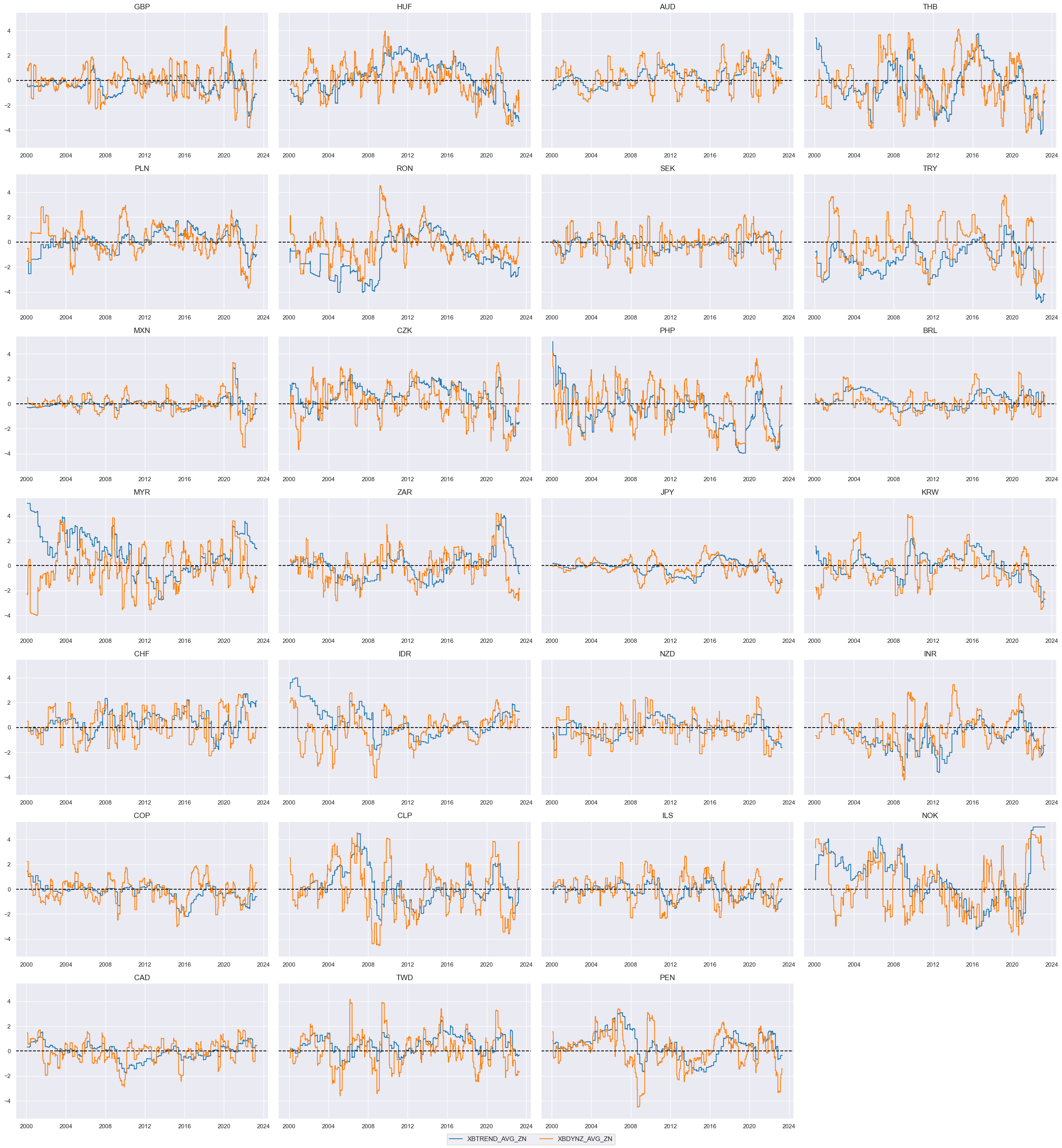
Next, we normalize values across both newly created trend and dynamics indicators
XBTREND_AVG
, and
XBDYNZ_AVG
. We compute z-scores for a category panel around zero, using monthly re-estimation frequency. For convenience and to be able to use potentially more indicators we create a dictionary of indicators using “T” as an indicator for trend (long-term average external ratios) and “D” for dynamics (short-term external ratio changes). To distinguish modified z-scored indicators from previously created ones, the newly created indicators receive postfix
_ZN
(
XBDYNZ_AVG_ZN
and
XBTREND_AVG_ZN
)
d_xs = {
    "T": "XBTREND_AVG",
    "D": "XBDYNZ_AVG",
}

xcatx = d_xs.values()
cidx = cids_fx

dfa = pd.DataFrame(columns=dfx.columns)
for xc in xcatx:
    dfaa = msp.make_zn_scores(
        dfx,
        xcat=xc,
        cids=cidx,
        sequential=True,
        min_obs=522,  # oos scaling after 2 years of panel data
        est_freq="m",
        neutral="zero",
        pan_weight=1,
        thresh=5,
        postfix="_ZN",
    )
    dfa = msm.update_df(dfa, dfaa)
dfx = msm.update_df(dfx, dfa)
xcatx = [xc + "_ZN" for xc in d_xs.values()]
cidx = cids_fx

msp.view_timelines(
    dfx,
    xcats=xcatx,
    cids=cidx,
    ncol=4,
    cumsum=False,
    start="2000-01-01",
    same_y=True,
    size=(12, 12),
    all_xticks=True,
  )
Here we create possible linear combinations of the two factors and call them
XSD_ZC
,
XSTD_ZC
, and
XST_ZC
. These combinations are effectively possible averages
# Collect all cycle external strength key combinations, i.e. T, D, TD (Trend, Dynamics, Trend+Dynamics)

xs_combs = [combo for r in range(1, 3) for combo in combinations(d_xs.keys(), r)]

# Use key combinations to calculate all possible factor combinations

dfa = pd.DataFrame(columns=dfx.columns).reindex([])

for xs in xs_combs:
    xcatx = [
        d_xs[i] + "_ZN" for i in xs
    ]  # extract absolute or relative category combination
    cidx = cids_fx
    dfaa = msp.linear_composite(
        dfx,
        xcats=xcatx,
        cids=cidx,
        complete_xcats=False,  # if some categories are missing the score is based on the remaining categories
        new_xcat="XS" + "".join(xs) + "_ZC",
    )
    dfa = msm.update_df(dfa, dfaa)

xszc = list(dfa["xcat"].unique())
dfx = msm.update_df(dfx, dfa)
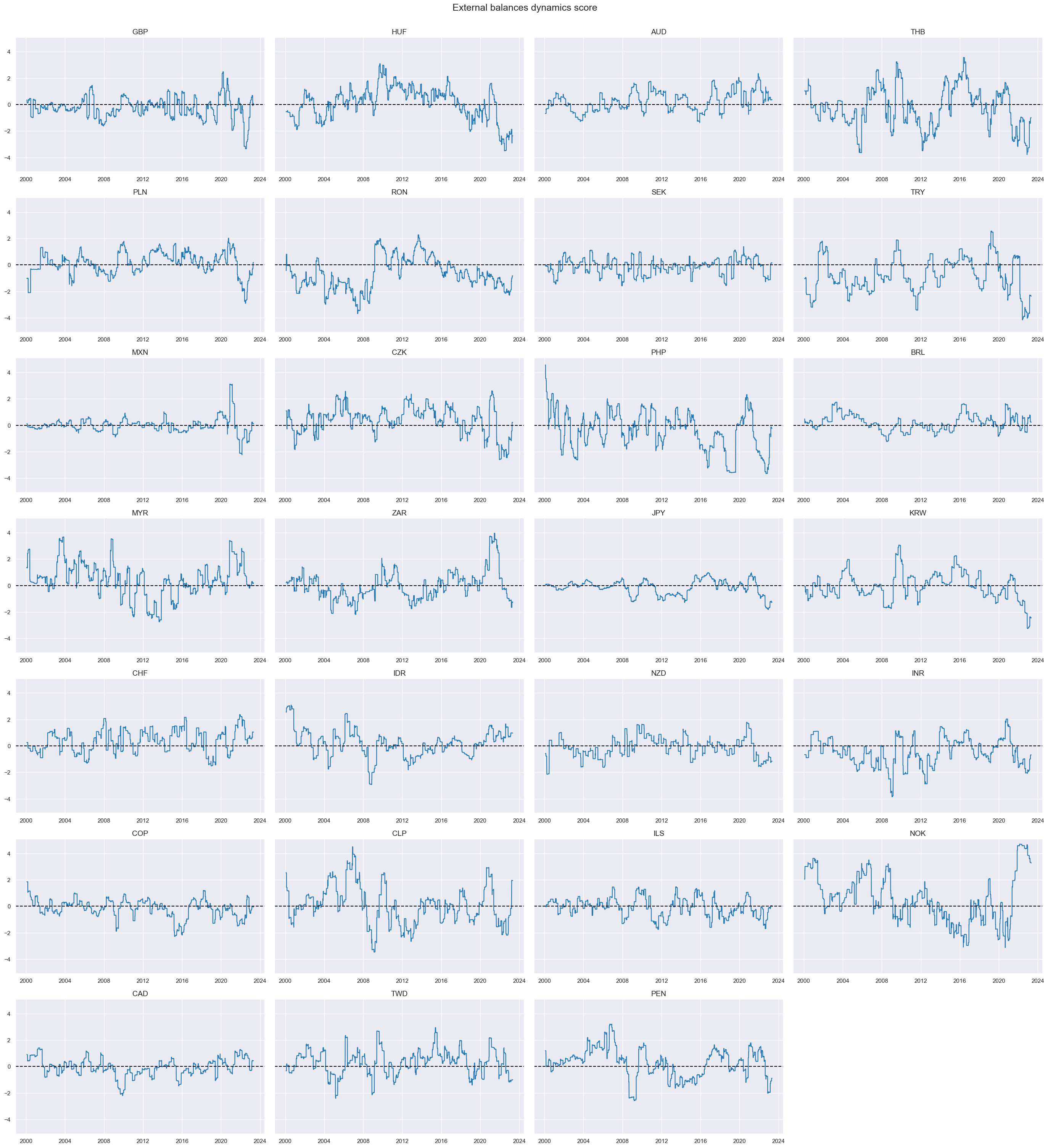
The following chart appears in the
post
. It displays composite z-score “external balance dynamics scores.” The series is naturally stationary, but positive and negative periods can last over several years, and variance has differed notably across countries. The indicator
XSTD_ZC
is the main indicator for the external balance dynamics score used in the post
# xcatx = ['XST_ZC', 'XSD_ZC', 'XSTD_ZC']
xcatx = ["XSTD_ZC"]
cidx = cids_fx

msp.view_timelines(
    dfx,
    xcats=xcatx,
    cids=cidx,
    ncol=4,
    cumsum=False,
    start="2000-01-01",
    same_y=True,
    size=(12, 12),
    all_xticks=True,
    title="External balances dynamics score",

)
FX return momentum and modification #
Standard trend #
Constructing plausible FX trend indicators is an important step in analyzing currency movements. In this notebook, we construct the following indicators:
-
The cumulative sum of FX forward returns as a measure of the overall return or performance of the currency over that period. A positive cumulative sum suggests an upward trend, while a negative cumulative sum indicates a downward trend.
-
Mean of 50 and 200 days rolling average: This indicator calculates the average value of the FX rates over a rolling window of 50 and 200 days, respectively. Comparing the 50-day rolling average with the 200-day rolling average can indicate potential shifts in the trend. When the 50-day average crosses above the 200-day average, it is often considered a bullish signal, suggesting a potential uptrend, and vice versa for a bearish signal.
-
Difference between 50 and 200 days means: this difference can indicate the strength or momentum of the trend. A positive difference suggests a strengthening trend, while a negative difference indicates a weakening trend.
fxrs = [
    "FXXR_VT10",  # FX forward return for 10% vol target: dominant cross
    "FXXRHvGDRB_NSA",
]  # Return on FX forward, hedged against market direction risk

calcs = []
for fxr in fxrs:
    calc = [
        f"{fxr}I = ( {fxr} ).cumsum()",
        f"{fxr}I_50DMA = {fxr}I.rolling(50).mean()",
        f"{fxr}I_200DMA = {fxr}I.rolling(200).mean()",
        f"{fxr}I_50v200DMA = {fxr}I_50DMA - {fxr}I_200DMA",
    ]
    calcs += calc

dfa = msp.panel_calculator(dfx, calcs, cids=cidx, blacklist=fxblack)
dfx = msm.update_df(dfx, dfa)
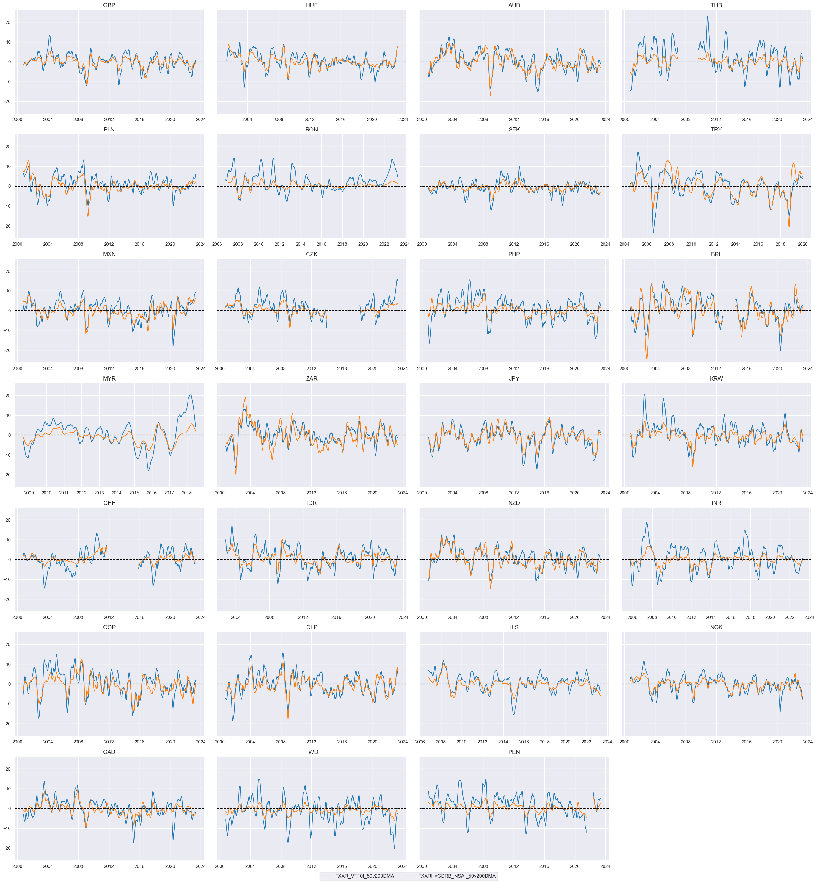
Here we choose two main FX trend indicators for the analysis:
-
The difference between 50 and 200 days means for FX forward return with a 10% vol target
FXXR_VT10I_50v200DMA: This indicator calculates the difference between the mean values of the FX forward returns over the 50-day and 200-day rolling windows. The returns used in this calculation are specific to FX forward contracts, and the indicator focuses on a 10% volatility target. Comparing the shorter-term average (50-day mean) with the longer-term average (200-day mean), gives an assessment of the relative strength or momentum of the trend. -
The difference between 50 and 200 days means for return on FX forward, hedged against market direction risk
FXXRHvGDRB_NSAI_50v200DMA
xcatx = ["FXXR_VT10I_50v200DMA", "FXXRHvGDRB_NSAI_50v200DMA"]
cidx = cids_fx

msp.view_timelines(
    dfx,
    xcats=xcatx,
    cids=cidx,
    ncol=4,
    cumsum=False,
    start="2000-01-01",
    same_y=True,
    size=(12, 12),
    all_xticks=True,

)
Modified trend #
In preparation for modification, we z-score both FX trends and previously constructed external trend scores with winsorization at 3 standard deviations. We add postfix
_Z3
to distinguish it from other indicators. For future analysis, we collect the normalized FX indicators in two separate lists: FX Trends in
trendz
(
FXVTREND_Z3
,
FXHTREND_Z3
) and external ratio indicators in list
xstrengthz
(
XSD_ZC_Z3
,
XSTD_ZC_Z3
,
XST_ZC_Z3
)
xcatx = ["FXXR_VT10I_50v200DMA", "FXXRHvGDRB_NSAI_50v200DMA"] + xszc
cidx = cids_fx

for xc in xcatx:
    dfaa = msp.make_zn_scores(
        dfx,
        xcat=xc,
        cids=cidx,
        sequential=True,
        min_obs=522,  # oos scaling after 2 years of panel data
        est_freq="m",
        neutral="zero",
        pan_weight=1,
        thresh=3,
        postfix="_Z3",
    )
    dfa = msm.update_df(dfa, dfaa)

dict_rename = {
    "FXXR_VT10I_50v200DMA": "FXVTREND",
    "FXXRHvGDRB_NSAI_50v200DMA": "FXHTREND",
}
dfa["xcat"] = dfa["xcat"].replace(dict_rename, regex=True)

dfx = msm.update_df(dfx, dfa)

trendz = [tr + "_Z3" for tr in list(dict_rename.values())]
xstrengthz = [xs + "_Z3" for xs in xszc]
Next, we apply a modification, allowing for adjustments to the strength of the FX trend signal based on the quantamental information captured by the external strength z-score. The FX return trend remains the dominant signal, but we allow quantamental information to increase the trend signal by up to 100% and to reduce it by up to zero. However, quantamental information does not “flip” the signal. The modification coefficient ensures that the adjustment remains within [0,2] interval, hence preventing extreme flips or amplifications of the trend signal.
The linear modification coefficient applied to the trend is based on the external strength z-score. The application depends on the sign of the concurrent trend signal.
-
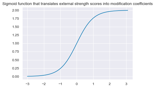
If the trend signal is positive, external strength enhances it and external weakness reduces it. The modification coefficient uses a sigmoid function that translates the external strength score such that for a value of zero it is 1, for values of -1 and 1 it is 0.25 and 1.75 respectively and for its minimum and maximum of -3 and 3 it is 0 zero and 2 respectively.
-
If the trend signal is negative the modification coefficient depends negatively on external strength in the same way.
This can be expressed in the following equation:
adtrend = ((1 - sign(external ratio trend))  + sign(external ratio trend) * coef) * trend

    where sign(external ratio trend) = 1 if external ratio trend >0; -1 if external ratio trend<0, and 0 if external ratio trend =0;
    coef = 2/(1 + exp(-2 * strength))
This means for positive trend:
adtrend = coef * external ratio trend
And this means for negative trend:
adtrend = (2 - coef) * external ratio trend
The modification coefficient for the trend signal is determined by a logistic (sigmoid) function of the external strength z-score. The modification coefficient can range between 0 and 2. Values larger than 1 strengthen the original signal, whereas values below one reduce the original signal.
def sigmoid(x):
    return 2 / (1 + np.exp(-2 * x))


ar = np.arange(-3, 3.2, 0.1)
plt.figure(figsize=(6, 4), dpi=80)
plt.plot(ar, sigmoid(ar))
plt.title(
    "Sigmoid function that translates external strength scores into modification coefficients"
)
plt.show()
We calculate the modification coefficients for all external strength scores, as applicable for positive trend scores, and then apply them to the trend scores in dependence on their signs. The coefficients get an additional postfix
_C
, so we get 3 series of coefficients based on the 3 external ratio z-scores created earlier (
XSD_ZC_Z3_C
,
XSTD_ZC_Z3_C
,
XST_ZC_Z3_C
)
calcs = []
for zd in xstrengthz:
    calcs += [f"{zd}_C = ( {zd} ).applymap( lambda x: 2 / (1 + np.exp( - 2 * x)) ) "]
dfa = msp.panel_calculator(dfx, calcs=calcs, cids=cidx)
dfx = msm.update_df(dfx, dfa)

coefs = list(dfa["xcat"].unique())
dfx[dfx["xcat"].isin(coefs)].head()  # to see the value of coefficients
| cid | xcat | real_date | value | |
|---|---|---|---|---|
| 224386 | AUD | XSD_ZC_Z3_C | 2000-02-01 | 0.472654 |
| 224387 | AUD | XSD_ZC_Z3_C | 2000-02-02 | 0.472654 |
| 224388 | AUD | XSD_ZC_Z3_C | 2000-02-03 | 0.472654 |
| 224389 | AUD | XSD_ZC_Z3_C | 2000-02-04 | 0.479073 |
| 224390 | AUD | XSD_ZC_Z3_C | 2000-02-07 | 0.479073 |
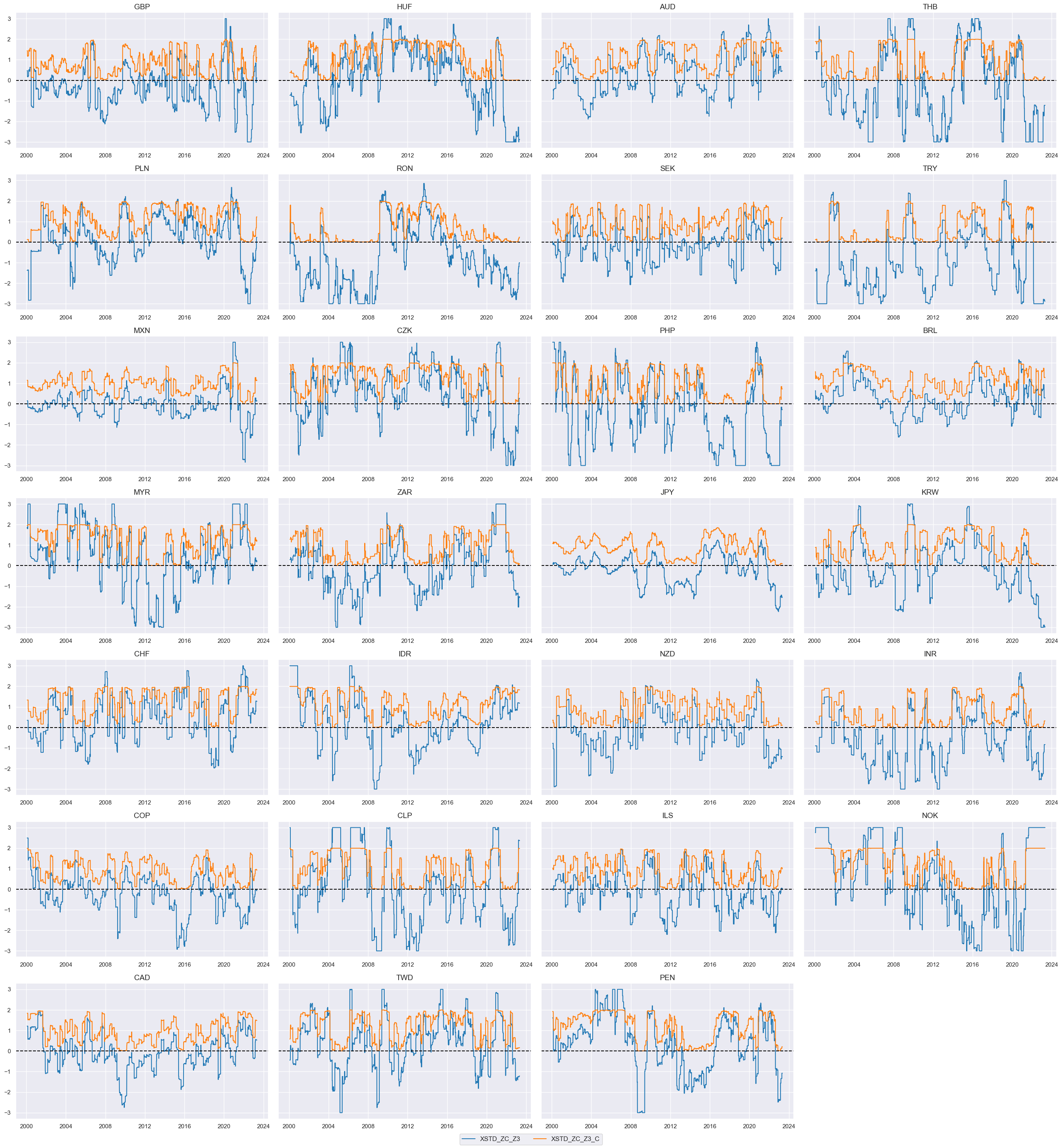
The charts below compare the original external strength scores with the sigmoid transformation coefficients. The coefficients are used to modify the trend scores, i.e. the higher the external strength the higher the trend score. The coefficients can only vary between 0 and 2.
xcatx = ["XSTD_ZC_Z3", "XSTD_ZC_Z3_C"]
cidx = cids_fx

msp.view_timelines(
    dfx,
    xcats=xcatx,
    cids=cidx,
    ncol=4,
    cumsum=False,
    start="2000-01-01",
    same_y=True,
    size=(12, 12),
    all_xticks=True,

)
The calculation of the trend sign-contingent coefficient and adjusted trends is based on the below formula.
((1 - sign(trend)) + sign(trend) * coef) * trend.
The new indicators will have the following structure in their name:
-
They will inherit
FXVorFXHfrom the first letters of the input FX indicatorFXVTREND_Z3(based on the original indicator FX forward return for 10% vol target: dominant cross), andFXHTREND_Z3(based on the original indicator Return on FX forward, hedged against market direction risk) -
they will have
min the name for ‘modified’ -
the name will have
XSD,XSTD, orXST` in its name indicating which of the external ratio indicators is used -
the coefficient names will end with
_Cpostfix to indicate that it is a coefficient or no postfix to indicate the modified indicator
For example,
FXVmXSTD_C
is a coefficient based on
FXVTREND_Z3
enhanced with Trend-dynamics external ratio scores
XSTD_ZC_Z3
. For convenience, the modified trend indicators are collected in the list
trendz_mod
calcs = []
for tr in trendz:
    for xs in xstrengthz:
        trxs = tr.split("TREND")[0] + "m" + xs.split("_")[0]
        calcs += [f"{trxs}_C = (1 - np.sign( {tr} )) + np.sign( {tr} ) * {xs}_C"]
        calcs += [f"{trxs} = {trxs}_C * {tr}"]

dfa = msp.panel_calculator(dfx, calcs=calcs, cids=cids_fx, blacklist=fxblack)
dfx = msm.update_df(dfx, dfa)

trendz_mod = [xc for xc in dfa["xcat"].unique() if not xc.endswith("_C")]
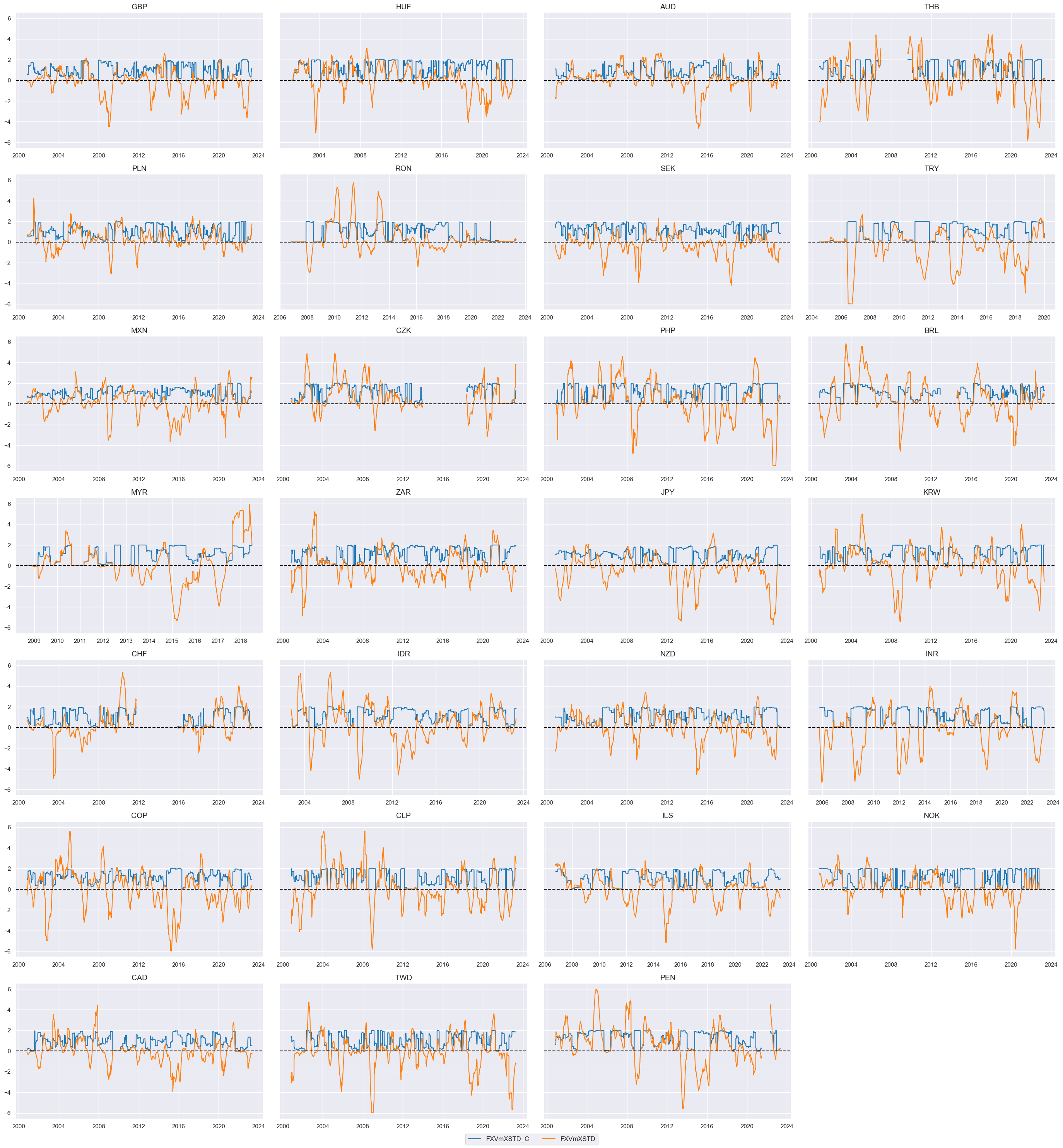
Here is a timeline of the coefficient for the composite indicator trend-dynamics and the modified indicator. As before, the value for the coefficient is between 0 and 2, with values below 1 mean reduction of the original signal and values above 1 mean strengthening of the original signal.
xcatx = ["FXVmXSTD_C", "FXVmXSTD"]
cidx = cids_fx

msp.view_timelines(
    dfx,
    xcats=xcatx,
    cids=cidx,
    ncol=4,
    cumsum=False,
    start="2000-01-01",
    same_y=True,
    size=(12, 12),
    all_xticks=True,

)
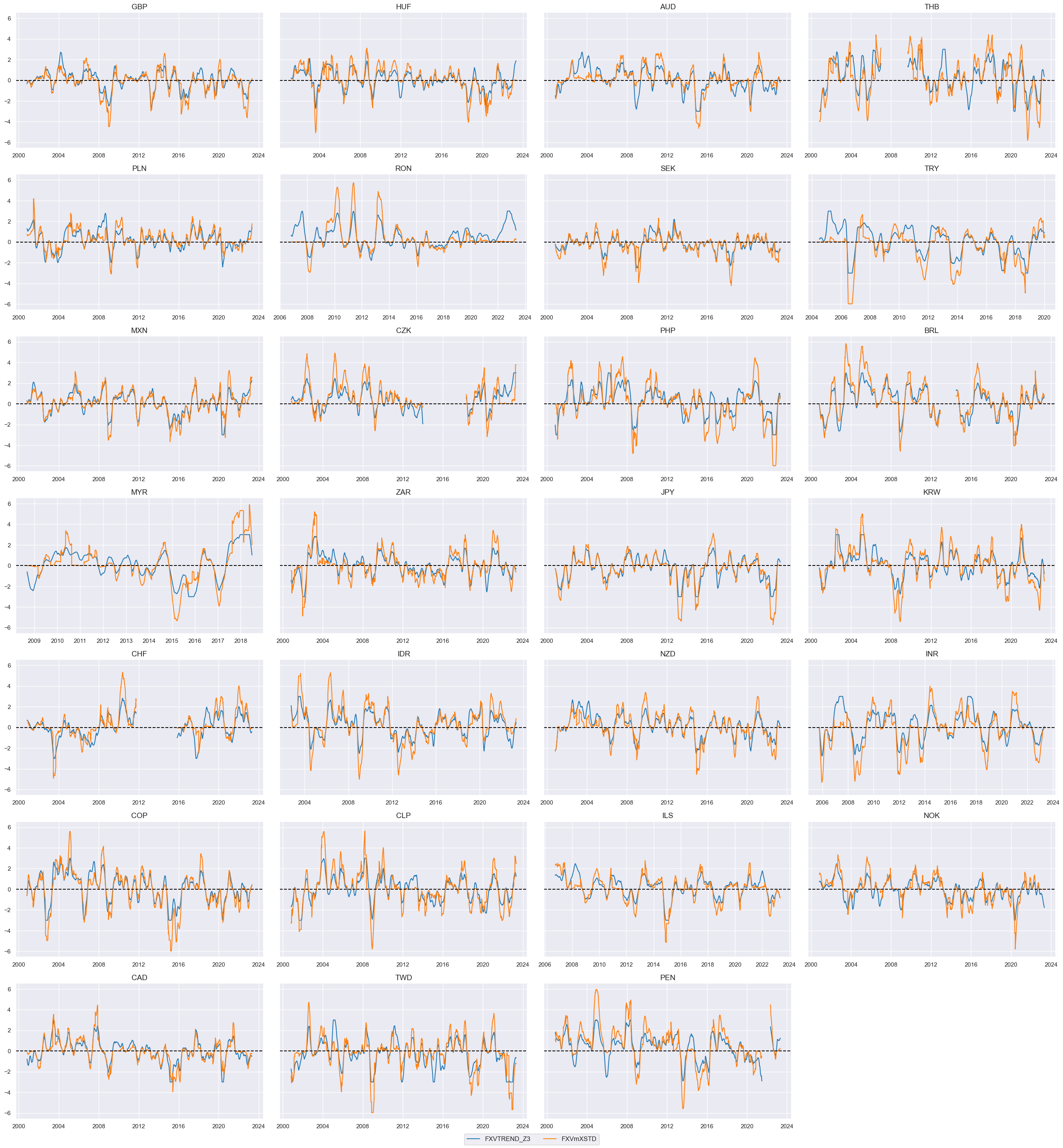
Here we compare the timeline of the modified FX trend indicator with the trend indicator created by multiplying it with external ratio adjustment.
xcatx = ["FXVTREND_Z3", "FXVmXSTD"]
cidx = cids_fx

msp.view_timelines(
    dfx,
    xcats=xcatx,
    cids=cidx,
    ncol=4,
    cumsum=False,
    start="2000-01-01",
    same_y=True,
    size=(12, 12),
    all_xticks=True,

)
Balanced trend #
A balanced trend here simply means that we sum up the trend and external strength z-scores. The new balanced indicators name will have the following structure:
-
They will inherit
FXVorFXHfrom the first letters of the input FX indicatorFXVTREND_Z3(based on the original indicator FX forward return for 10% vol target: dominant cross), andFXHTREND_Z3(based on the original indicator Return on FX forward, hedged against market direction risk) -
they will have
bin the name forbalanced -
the name will have
XSD,XSTD, orXST` in its name indicating which of the external ratio indicators is used
The new balanced indicators will be collected in a list
trendz_bal
for further analysis.
calcs = []
for tr in trendz:
    for xs in xstrengthz:
        trxs = tr.split("TREND")[0] + "b" + xs.split("_")[0]
        calcs += [f"{trxs} = ( {tr} + {xs} ) / 2"]

dfa = msp.panel_calculator(dfx, calcs=calcs, cids=cids_fx, blacklist=fxblack)
dfx = msm.update_df(dfx, dfa)

trendz_bal = [xc for xc in dfa["xcat"].unique() if not xc.endswith("_C")]
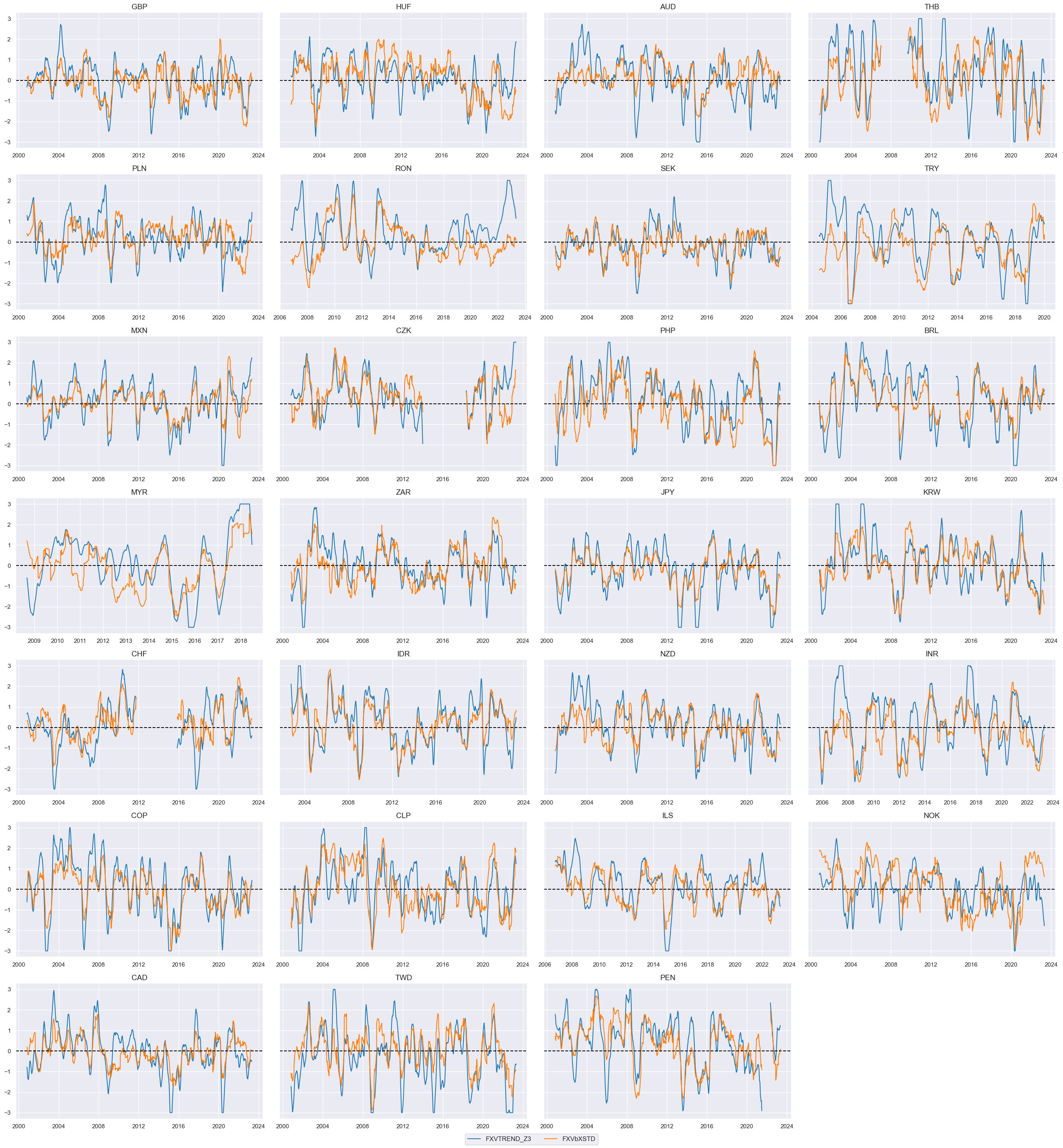
Here we compare the timelines for
FXVTREND_Z3
and the balanced indicator
FXVbXSTD
xcatx = ["FXVTREND_Z3", "FXVbXSTD"]
cidx = cids_fx

msp.view_timelines(
    dfx,
    xcats=xcatx,
    cids=cidx,
    ncol=4,
    cumsum=False,
    start="2000-01-01",
    same_y=True,
    size=(12, 12),
    all_xticks=True,

)
Relative scores #
Here we create relative values for original, modified, and balanced trend scores. The relative values are calculated by subtracting the mean of the score from the score itself. This is done to ensure that the model is not biased towards any particular value of the score. The name of the indicator will include
_vGFX
postfix for “versus Global FX” indicating that the average of the whole basket is taken for basis.
xcatx = trendz + trendz_mod + trendz_bal
dfa = msp.make_relative_value(
    dfx,
    xcats=xcatx,
    cids=cids_fx,
    start="2000-01-01",
    blacklist=fxblack,
    rel_meth="subtract",
    postfix="vGFX",
)
dfx = msm.update_df(dfx, dfa)
dfa["xcat"].unique()
array(['FXHTREND_Z3vGFX', 'FXHbXSDvGFX', 'FXHbXSTvGFX', 'FXHbXSTDvGFX',
       'FXHmXSDvGFX', 'FXHmXSTvGFX', 'FXHmXSTDvGFX', 'FXVTREND_Z3vGFX',
       'FXVbXSDvGFX', 'FXVbXSTvGFX', 'FXVbXSTDvGFX', 'FXVmXSDvGFX',
       'FXVmXSTvGFX', 'FXVmXSTDvGFX'], dtype=object)
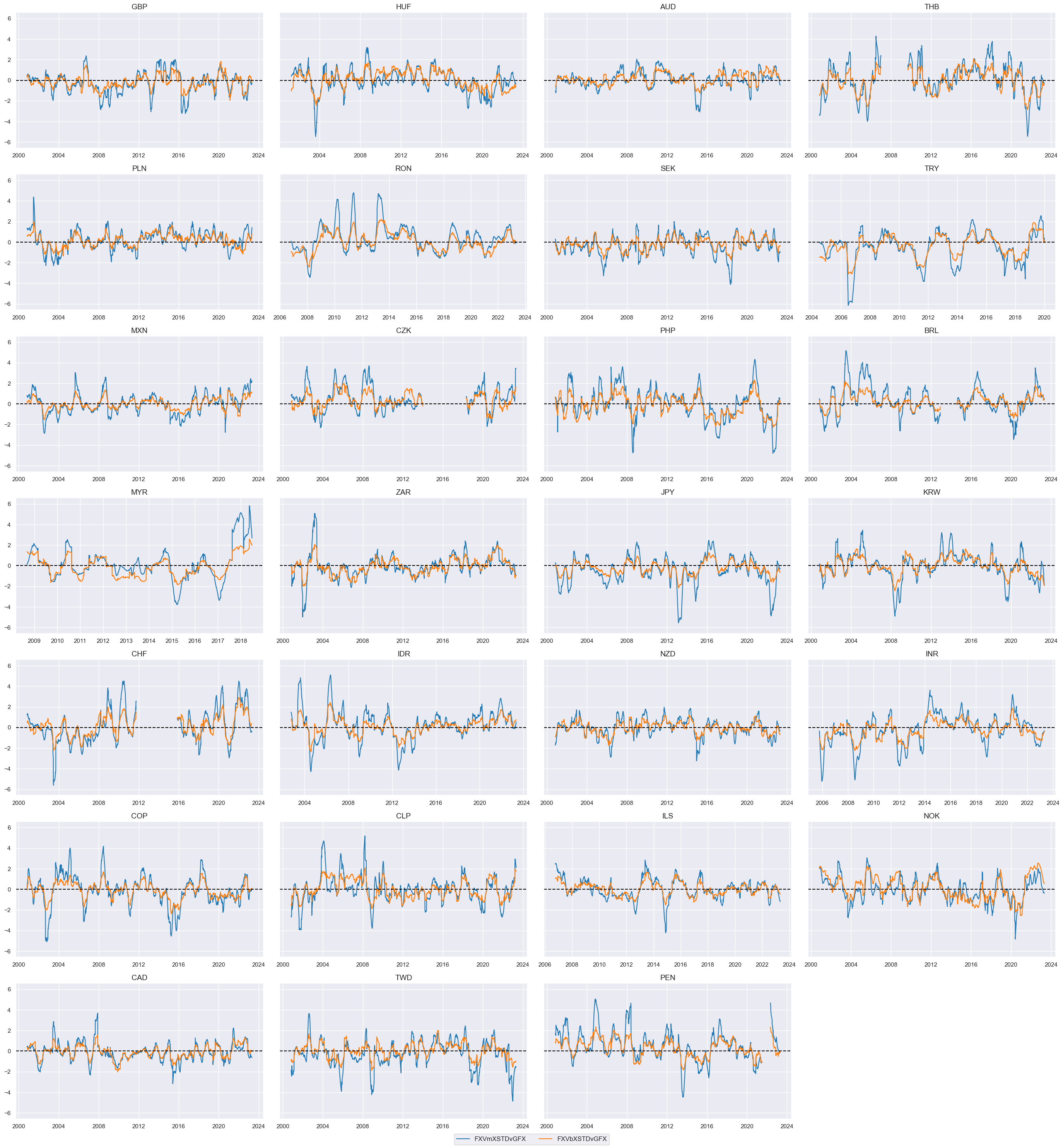
We compare the performance of the two trends, the modified and the balanced models.
xcatx = ["FXVmXSTDvGFX", "FXVbXSTDvGFX"]
cidx = cids_fx

msp.view_timelines(
    dfx,
    xcats=xcatx,
    cids=cidx,
    ncol=4,
    cumsum=False,
    start="2000-01-01",
    same_y=True,
    size=(12, 12),
    all_xticks=True,
   )
The same relative value is calculated for each EM currency versus an EM average and postfix
vEFX
is added to these indicators.
xcatx = trendz + trendz_mod + trendz_bal
dfa = msp.make_relative_value(
    dfx,
    xcats=xcatx,
    cids=cids_emfx,
    start="2000-01-01",
    blacklist=fxblack,
    rel_meth="subtract",
    postfix="vEFX",
)
dfx = msm.update_df(dfx, dfa)
dfa["xcat"].unique()
array(['FXHTREND_Z3vEFX', 'FXHbXSDvEFX', 'FXHbXSTvEFX', 'FXHbXSTDvEFX',
       'FXHmXSDvEFX', 'FXHmXSTvEFX', 'FXHmXSTDvEFX', 'FXVTREND_Z3vEFX',
       'FXVbXSDvEFX', 'FXVbXSTvEFX', 'FXVbXSTDvEFX', 'FXVmXSDvEFX',
       'FXVmXSTvEFX', 'FXVmXSTDvEFX'], dtype=object)
Targets #
Types of FX return #
Directional vol-targeted and hedged returns #
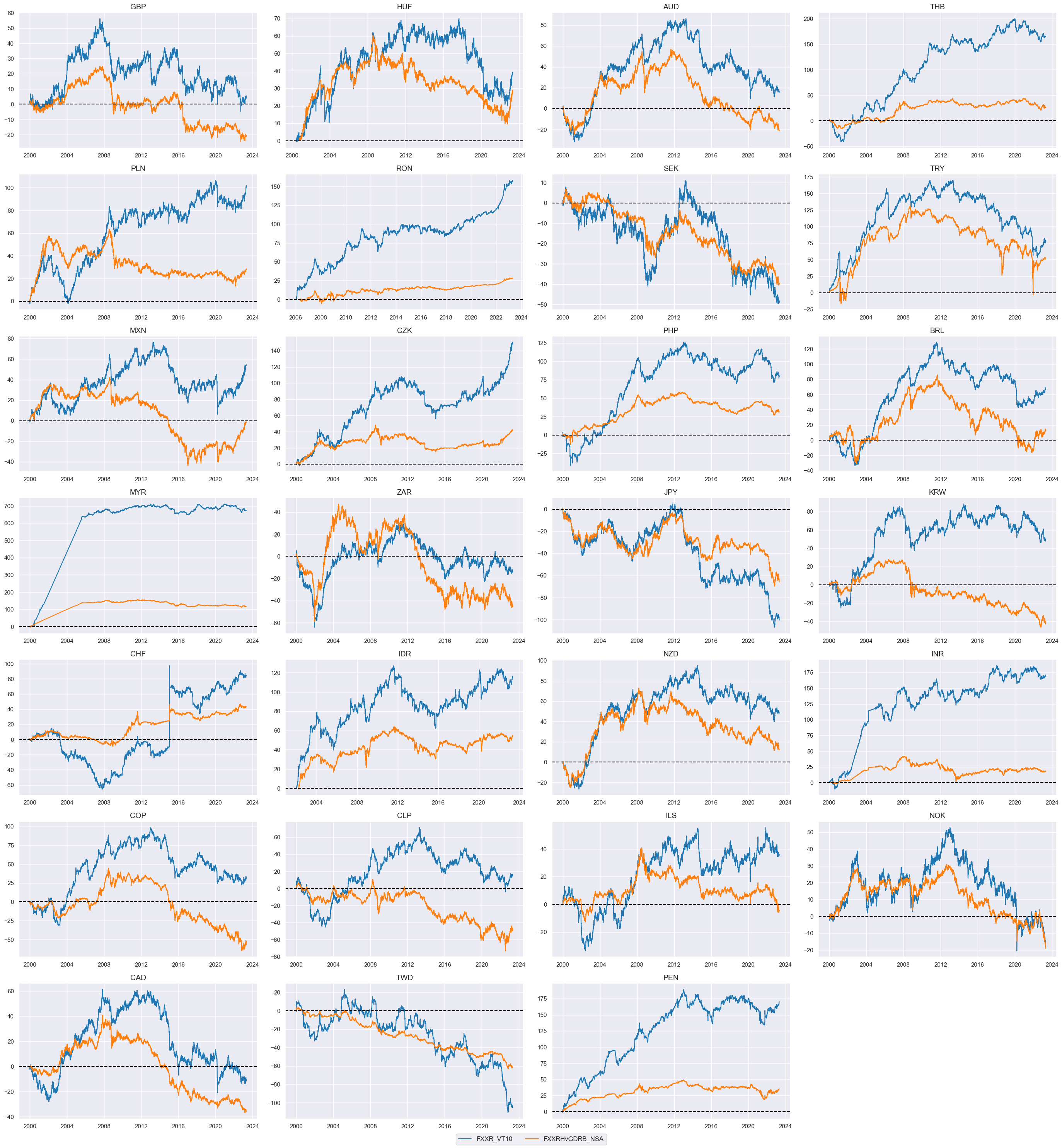
We are taking here, as before, 2 FX returns: cumulative FX forward return for 10% vol target: dominant cross
FXXR_VT10
and cumulative return on FX forward, hedged against market direction risk
FXXRHvGDRB_NSA
xcatx = ["FXXR_VT10", "FXXRHvGDRB_NSA"]
cidx = cids_fx

msp.view_timelines(
    dfx,
    xcats=xcatx,
    cids=cidx,
    ncol=4,
    cumsum=True,
    start="2000-01-01",
    same_y=False,
    size=(12, 12),
    all_xticks=True,
    title=None,
    xcat_labels=None,
)
Global relative returns #
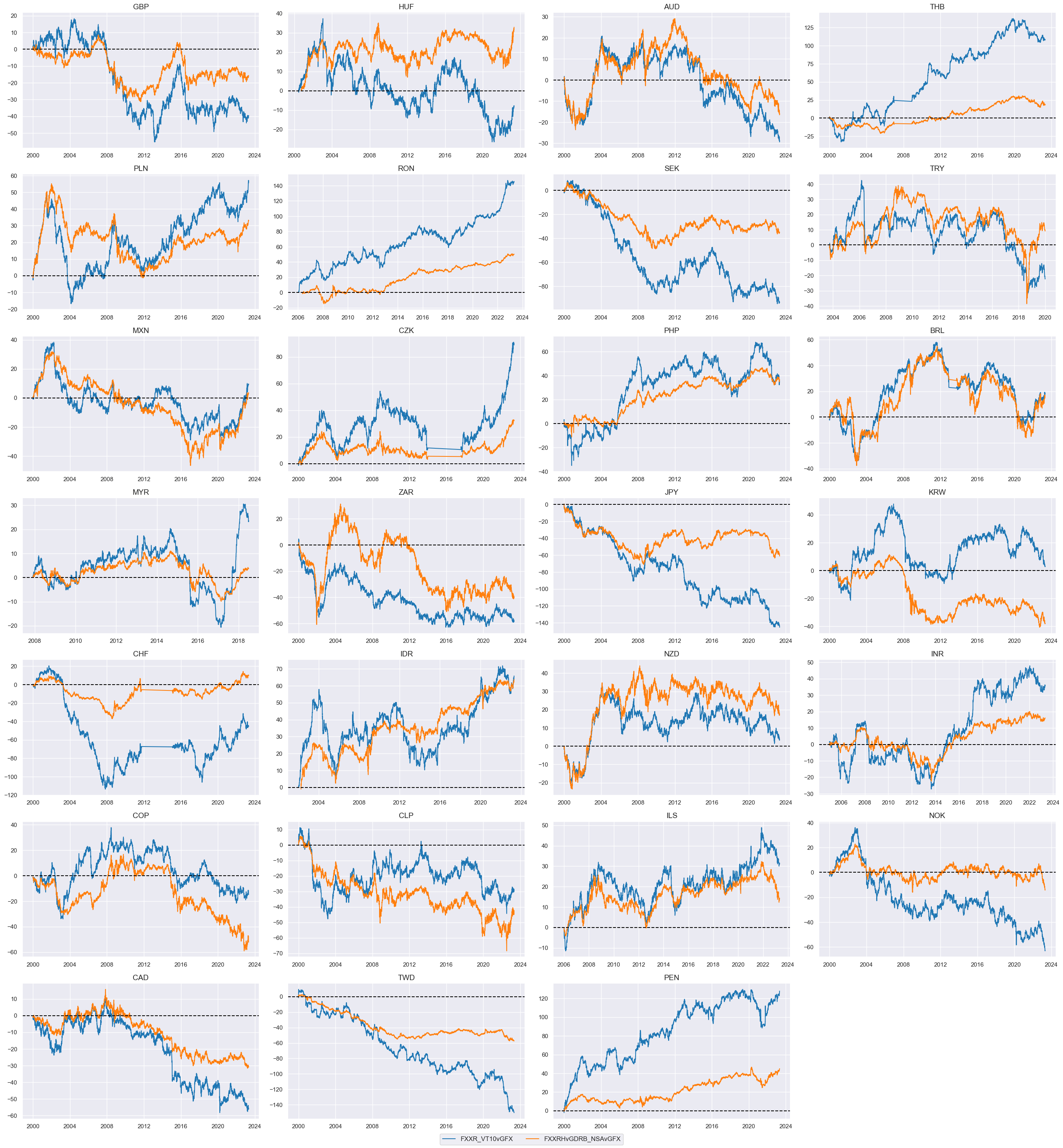
We calculate the relative value for unhedged and hedged FX forward returns by subtracting the panel average from each individual category.
xcatx = ["FXXR_VT10", "FXXRHvGDRB_NSA"]
dfa = msp.make_relative_value(
    dfx,
    xcats=xcatx,
    cids=cids_fx,
    start="2000-01-01",
    blacklist=fxblack,
    rel_meth="subtract",
    postfix="vGFX",
)
dfx = msm.update_df(dfx, dfa)
visualizing selected relative value indicators on a timeline:
xcatx = ["FXXR_VT10vGFX", "FXXRHvGDRB_NSAvGFX"]
cidx = cids_fx

msp.view_timelines(
    dfx,
    xcats=xcatx,
    cids=cidx,
    ncol=4,
    cumsum=True,
    start="2000-01-01",
    same_y=False,
    size=(12, 12),
    all_xticks=True,
    title=None,
    xcat_labels=None,
)
EM relative returns #
The same calculations can be done for emerging market currencies.
xcatx = ["FXXR_VT10", "FXXRHvGDRB_NSA"]
cidx = cids_emfx

dfa = msp.make_relative_value(
    dfx,
    xcats=xcatx,
    cids=cids_fx,
    start="2000-01-01",
    blacklist=fxblack,
    rel_meth="subtract",
    postfix="vEFX",
)
dfx = msm.update_df(dfx, dfa)
xcatx = ["FXXR_VT10vEFX", "FXXRHvGDRB_NSAvEFX"]
cidx = cids_fx

msp.view_timelines(
    dfx,
    xcats=xcatx,
    cids=cidx,
    ncol=4,
    cumsum=True,
    start="2000-01-01",
    same_y=False,
    size=(12, 12),
    all_xticks=True,
    title=None,
    xcat_labels=None,
)

Value checks #
Standard trend following #
Specs and panel test #
Here we specify the target variable and the list of signals (defined earlier in the list
trendz
, consisting of
FXVTREND_Z3
and
FXHTREND_Z3
) to use as predictors. As the main signal, to use later as a benchmark, we use the original z-score of unhedged FX forward return
FXVTREND_Z3
(non-modified and not-balanced)
sigs = trendz
ms = "FXVTREND_Z3"  # main signal
oths = list(set(sigs) - set([ms]))  # other signals

targ = "FXXR_VT10"
cidx = cids_fx

dict_trend = {
    "sig": ms,
    "rivs": oths,
    "targ": targ,
    "cidx": cidx,
    "black": fxblack,
    "srr": None,
    "pnls": None,
}
Utilizing ‘CategoryRelations’ function from the
Macrosynergy package
, we specify a lag of one month for the main signal (
FXVTREND_Z3
), frequency, start dates and apply blacklist periods to the analysis.
dix = dict_trend

sig = dix["sig"]
targ = dix["targ"]
cidx = dix["cidx"]
blax = dix["black"]

crx = msp.CategoryRelations(
    dfx,
    xcats=[sig, targ],
    cids=cidx,
    freq="M",
    lag=1,
    xcat_aggs=["last", "sum"],
    start="2002-01-01",
    blacklist=blax,
    xcat_trims=[None, None],
)
crx.reg_scatter(
    labels=False,
    coef_box="lower left",
    # separator=2010,
    xlab=None,
    ylab=None,
    title=None,
    size=(10, 6),
    prob_est="map",
)
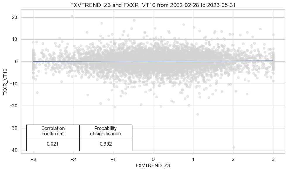
Accuracy and correlation check #
Another useful function from the Macrosynergy package analyses and compares the relationships between the chosen signals and the panel of subsequent returns. There is no regression analysis involved, rather the sign of the signal is used for predicting the sign of the target.
dix = dict_trend

sig = dix["sig"]
rivs = dix["rivs"]
targ = dix["targ"]
cidx = dix["cidx"]
blax = dix["black"]

srr = mss.SignalReturnRelations(
    dfx,
    cids=cidx,
    sigs=[sig] + rivs,
    rets=targ,
    freqs="M",
    start="2002-01-01",
    blacklist=blax,
)

dix["srr"] = srr
The Summary table below gives a short high-level snapshot of the strength and stability of the main signal relation.
dix = dict_trend
srrx = dix["srr"]
display(srrx.summary_table().sort_index().astype("float").round(3))
| accuracy | bal_accuracy | pos_sigr | pos_retr | pos_prec | neg_prec | pearson | pearson_pval | kendall | kendall_pval | auc | |
|---|---|---|---|---|---|---|---|---|---|---|---|
| M: FXVTREND_Z3/last => FXXR_VT10 | 0.525 | 0.520 | 0.566 | 0.546 | 0.563 | 0.477 | 0.021 | 0.091 | 0.028 | 0.001 | 0.520 |
| Mean cids | 0.527 | 0.517 | 0.568 | 0.547 | 0.560 | 0.474 | 0.012 | 0.573 | 0.017 | 0.566 | 0.516 |
| Mean years | 0.526 | 0.508 | 0.567 | 0.546 | 0.550 | 0.466 | -0.018 | 0.321 | -0.002 | 0.348 | 0.506 |
| Positive ratio | 0.773 | 0.636 | 0.773 | 0.682 | 0.727 | 0.273 | 0.318 | 0.273 | 0.409 | 0.318 | 0.636 |
| Positive ratio | 0.741 | 0.667 | 0.852 | 0.852 | 0.889 | 0.185 | 0.556 | 0.185 | 0.667 | 0.333 | 0.667 |
The signals table gives an overview of the signal-return relationship across the main and rival signals, which produce a very similar result in our case:
dix = dict_trend
srrx = dix["srr"]
display(srrx.signals_table().sort_index().astype("float").round(3))
| accuracy | bal_accuracy | pos_sigr | pos_retr | pos_prec | neg_prec | pearson | pearson_pval | kendall | kendall_pval | auc | ||||
|---|---|---|---|---|---|---|---|---|---|---|---|---|---|---|
| Return | Signal | Frequency | Aggregation | |||||||||||
| FXXR_VT10 | FXHTREND_Z3 | M | last | 0.526 | 0.527 | 0.490 | 0.545 | 0.573 | 0.481 | 0.024 | 0.052 | 0.030 | 0.000 | 0.527 |
| FXVTREND_Z3 | M | last | 0.525 | 0.520 | 0.566 | 0.546 | 0.563 | 0.477 | 0.021 | 0.091 | 0.028 | 0.001 | 0.520 |
Naive PnL #
Here we calculate a daily PnL for selected signals ‘FXVTREND_Z3’ and ‘FXHTREND_Z3’. We create a new PnL series with postfix
_PZN
to indicate that the raw signal has been transformed into z-scores. In the cell below two PnL series are created:
FXVTREND_Z3_PZN
, and
              Long


              only
dix = dict_trend

sigx = [dix["sig"]] + dix["rivs"]
targ = dix["targ"]
cidx = dix["cidx"]
blax = dix["black"]

naive_pnl = msn.NaivePnL(
    dfx,
    ret=targ,
    sigs=sigx,
    cids=cidx,
    start="2000-01-01",
    blacklist=blax,
    bms=["USD_EQXR_NSA"],
)

for sig in sigx:
    naive_pnl.make_pnl(
        sig,
        sig_neg=False,
        sig_op="zn_score_pan",
        thresh=3,
        rebal_freq="monthly",
        vol_scale=10,
        rebal_slip=1,
        pnl_name=sig + "_PZN",
    )


naive_pnl.make_long_pnl(vol_scale=10, label="Long only")
dix["pnls"] = naive_pnl
We plot both PnL series to compare with each other
dix = dict_trend

sigx = dix["sig"]
naive_pnl = dix["pnls"]
pnls = [sigx + x for x in ["_PZN"]] + ["Long only"]

naive_pnl.plot_pnls(
    pnl_cats=pnls,
    pnl_cids=["ALL"],
    start="2001-01-01",
    title=None,
    xcat_labels=None,
    figsize=(16, 8),
)
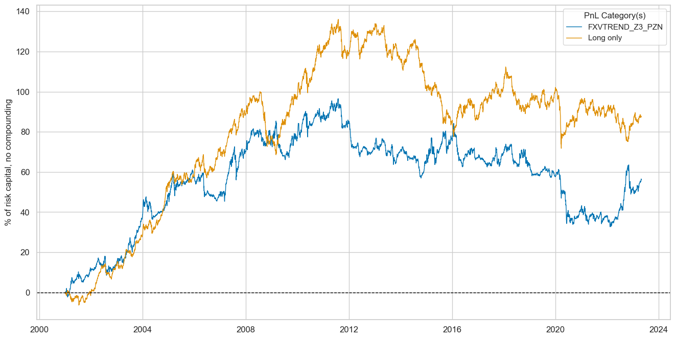
and display basic statistics, including the return, standard deviation, and sharpe ratio
dix = dict_trend

sigx = [dix["sig"]] + dix["rivs"]
naive_pnl = dix["pnls"]
pnls = [sig + type for sig in sigx for type in ["_PZN"]]

df_eval = naive_pnl.evaluate_pnls(
    pnl_cats=pnls,
    pnl_cids=["ALL"],
    start="2000-01-01",
)
display(df_eval.transpose())
| Return % | St. Dev. % | Sharpe Ratio | Sortino Ratio | Max 21-Day Draw % | Max 6-Month Draw % | Peak to Trough Draw % | Top 5% Monthly PnL Share | USD_EQXR_NSA correl | Traded Months | |
|---|---|---|---|---|---|---|---|---|---|---|
| xcat | ||||||||||
| FXVTREND_Z3_PZN | 2.450134 | 10.0 | 0.245013 | 0.330989 | -15.695437 | -25.215399 | -63.816973 | 1.620189 | 0.003897 | 272 |
| FXHTREND_Z3_PZN | 2.722056 | 10.0 | 0.272206 | 0.380782 | -18.527208 | -23.223193 | -45.321138 | 1.665439 | -0.033459 | 272 |
Both original z-score FX trend indicators produce very similar statistics for the observed period. In fact, the long-only strategy seems to outperform both signals most of the time.
External balance strength #
Specs and panel test #
Here we use external balance strength indicators as signals. The main signal will be the external balances dynamics score
XSTD_ZC_Z3
sigs = xstrengthz
ms = "XSTD_ZC_Z3"  # main signal
oths = list(set(sigs) - set([ms])) + ["FXVTREND_Z3"]  # other signals

targ = "FXXR_VT10"
cidx = cids_fx

dict_xs = {
    "sig": ms,
    "rivs": oths,
    "targ": targ,
    "cidx": cidx,
    "black": fxblack,
    "srr": None,
    "pnls": None,
}
dix = dict_xs

sig = dix["sig"]
targ = dix["targ"]
cidx = dix["cidx"]
blax = dix["black"]

crx = msp.CategoryRelations(
    dfx,
    xcats=[sig, targ],
    cids=cidx,
    freq="M",
    lag=1,
    xcat_aggs=["last", "sum"],
    start="2000-01-01",
    blacklist=blax,
    xcat_trims=[None, None],
)
crx.reg_scatter(
    labels=False,
    coef_box="lower left",
    # separator=2010,
    xlab=None,
    ylab=None,
    title=None,
    size=(10, 6),
    prob_est="map",
)
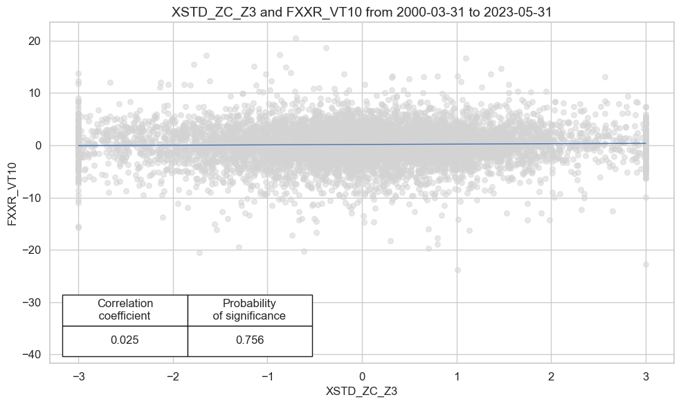
Accuracy and correlation bars #
dix = dict_xs

sig = dix["sig"]
rivs = dix["rivs"]
targ = dix["targ"]
cidx = dix["cidx"]
blax = dix["black"]

srr = mss.SignalReturnRelations(
    dfx,
    cids=cidx,
    sigs=[sig] + rivs,
    rets=targ,
    freqs="M",
    start="2000-01-01",
    blacklist=blax,
)

dix["srr"] = srr
dix = dict_xs
srrx = dix["srr"]
display(srrx.summary_table().sort_index().astype("float").round(3))
| accuracy | bal_accuracy | pos_sigr | pos_retr | pos_prec | neg_prec | pearson | pearson_pval | kendall | kendall_pval | auc | |
|---|---|---|---|---|---|---|---|---|---|---|---|
| M: XSTD_ZC_Z3/last => FXXR_VT10 | 0.512 | 0.512 | 0.496 | 0.544 | 0.556 | 0.468 | 0.025 | 0.038 | 0.019 | 0.018 | 0.512 |
| Mean cids | 0.511 | 0.514 | 0.492 | 0.546 | 0.561 | 0.466 | 0.029 | 0.417 | 0.020 | 0.428 | 0.513 |
| Mean years | 0.509 | 0.505 | 0.493 | 0.544 | 0.548 | 0.462 | 0.010 | 0.437 | 0.007 | 0.381 | 0.505 |
| Positive ratio | 0.583 | 0.542 | 0.500 | 0.667 | 0.708 | 0.333 | 0.667 | 0.375 | 0.542 | 0.417 | 0.542 |
| Positive ratio | 0.630 | 0.667 | 0.370 | 0.889 | 0.778 | 0.185 | 0.667 | 0.444 | 0.667 | 0.519 | 0.667 |
The table below compares accuracy, balanced accuracy, positive and negative precisions for external ratio scores and for the original FX trend score.
dix = dict_xs
srrx = dix["srr"]
display(srrx.signals_table().sort_index().astype("float").round(3))
| accuracy | bal_accuracy | pos_sigr | pos_retr | pos_prec | neg_prec | pearson | pearson_pval | kendall | kendall_pval | auc | ||||
|---|---|---|---|---|---|---|---|---|---|---|---|---|---|---|
| Return | Signal | Frequency | Aggregation | |||||||||||
| FXXR_VT10 | FXVTREND_Z3 | M | last | 0.528 | 0.523 | 0.558 | 0.545 | 0.565 | 0.480 | 0.024 | 0.048 | 0.032 | 0.000 | 0.523 |
| XSD_ZC_Z3 | M | last | 0.510 | 0.510 | 0.499 | 0.544 | 0.554 | 0.466 | 0.028 | 0.018 | 0.018 | 0.021 | 0.510 | |
| XSTD_ZC_Z3 | M | last | 0.512 | 0.512 | 0.496 | 0.544 | 0.556 | 0.468 | 0.025 | 0.038 | 0.019 | 0.018 | 0.512 | |
| XST_ZC_Z3 | M | last | 0.506 | 0.506 | 0.497 | 0.544 | 0.550 | 0.461 | 0.013 | 0.281 | 0.010 | 0.235 | 0.506 |
Naive PnLs #
dix = dict_xs

sigx = [dix["sig"]] + dix["rivs"]
targ = dix["targ"]
cidx = dix["cidx"]
blax = dix["black"]

naive_pnl = msn.NaivePnL(
    dfx,
    ret=targ,
    sigs=sigx,
    cids=cidx,
    start="2002-01-01",
    blacklist=blax,
    bms=["USD_EQXR_NSA"],
)

for sig in sigx:
    naive_pnl.make_pnl(
        sig,
        sig_neg=False,
        sig_op="zn_score_pan",
        thresh=2,
        rebal_freq="monthly",
        vol_scale=10,
        rebal_slip=1,
        pnl_name=sig + "_PZN",
    )

dix["pnls"] = naive_pnl
In this plot, we compare two PnLs based on:
-
based on the Standard 50-day versus 200 day trend score and
-
external balance dynamics score
dix = dict_xs

sigx = ["FXVTREND_Z3"] + [dix["sig"]]
naive_pnl = dix["pnls"]
pnls = [sig + "_PZN" for sig in sigx]
dict_labels = {"FXVTREND_Z3_PZN": "Standard 50-day versus 200 day trend score", "XSTD_ZC_Z3_PZN": "External balance dynamics score"}


naive_pnl.plot_pnls(
    pnl_cats=pnls,
    pnl_cids=["ALL"],
    start="2002-01-01",
    title="FX forward PnL (all DM and EM versus USD or EUR) based on trend and external balance dynamics",
    xcat_labels=dict_labels,
    figsize=(16, 8),
)
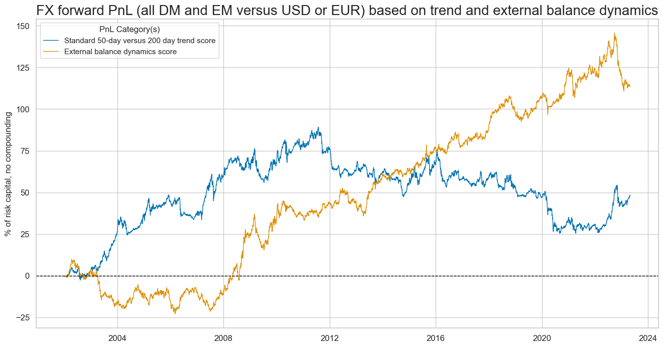
These naïve PnLs suggest that the economic value of the external dynamics score (Sharpe 0.42 - see table below) has been greater than that of the trend score (Sharpe 0.19). More importantly, the two have been highly complementary. While the trend signal produced all its value in the 2000s, the external dynamics score produced consistent positive returns from 2008 to 2022.
We can also compare the performance of the trend and external balance signals in terms of their returns, Sharpe ratios, maximum 21 day draw, and correlation with the benchmark
dix = dict_xs

sigx = [dix["sig"]] + dix["rivs"]
naive_pnl = dix["pnls"]
pnls = [sig + "_PZN" for sig in sigx]

df_eval = naive_pnl.evaluate_pnls(
    pnl_cats=pnls,
    pnl_cids=["ALL"],
    start="2002-01-01",
)
display(df_eval.transpose())
| Return % | St. Dev. % | Sharpe Ratio | Sortino Ratio | Max 21-Day Draw % | Max 6-Month Draw % | Peak to Trough Draw % | Top 5% Monthly PnL Share | USD_EQXR_NSA correl | Traded Months | |
|---|---|---|---|---|---|---|---|---|---|---|
| xcat | ||||||||||
| XSTD_ZC_Z3_PZN | 5.337542 | 10.0 | 0.533754 | 0.770637 | -16.808909 | -33.075748 | -34.869693 | 0.95083 | -0.065803 | 257 |
| XSD_ZC_Z3_PZN | 4.707322 | 10.0 | 0.470732 | 0.683301 | -17.057686 | -26.751891 | -40.978567 | 1.080764 | -0.050714 | 257 |
| XST_ZC_Z3_PZN | 4.45383 | 10.0 | 0.445383 | 0.64153 | -14.369015 | -36.340876 | -36.972571 | 1.146386 | -0.078699 | 257 |
| FXVTREND_Z3_PZN | 2.254828 | 10.0 | 0.225483 | 0.305464 | -14.177166 | -23.03066 | -63.655385 | 1.717695 | 0.010921 | 257 |
Modified trend following #
Specs and panel test #
Here we take the modified signal
FXVmXSTD
and evaluate it in the context of the other signals.
sigs = [tr for tr in trendz_mod if tr.startswith("FXV")] + ["FXVTREND_Z3"]
ms = "FXVmXSTD"  # main signal
oths = list(set(sigs) - set([ms]))  # other signals

targ = "FXXR_VT10"
cidx = cids_fx

dict_xsmod = {
    "sig": ms,
    "rivs": oths,
    "targ": targ,
    "cidx": cidx,
    "black": fxblack,
    "srr": None,
    "pnls": None,
}
dix = dict_xsmod

sig = dix["sig"]
targ = dix["targ"]
cidx = dix["cidx"]
blax = dix["black"]

crx = msp.CategoryRelations(
    dfx,
    xcats=[sig, targ],
    cids=cidx,
    freq="M",
    lag=1,
    slip=1,
    xcat_aggs=["last", "sum"],
    start="2002-01-01",
    blacklist=blax,
    xcat_trims=[None, None],
)
crx.reg_scatter(
    labels=False,
    coef_box="lower left",
    # separator=2010,
    xlab=None,
    ylab=None,
    title=None,
    size=(10, 6),
    prob_est="map",
)
Accuracy and correlation bars #
dix = dict_xsmod

sig = dix["sig"]
rivs = dix["rivs"]
targ = dix["targ"]
cidx = dix["cidx"]
blax = dix["black"]

srr = mss.SignalReturnRelations(
    dfx,
    cids=cidx,
    sigs=[sig] + rivs,
    rets=targ,
    freqs="M",
    start="2002-01-01",
    blacklist=blax,
)

dix["srr"] = srr
dix = dict_xsmod
srrx = dix["srr"]
display(srrx.summary_table().sort_index().astype("float").round(3))
| accuracy | bal_accuracy | pos_sigr | pos_retr | pos_prec | neg_prec | pearson | pearson_pval | kendall | kendall_pval | auc | |
|---|---|---|---|---|---|---|---|---|---|---|---|
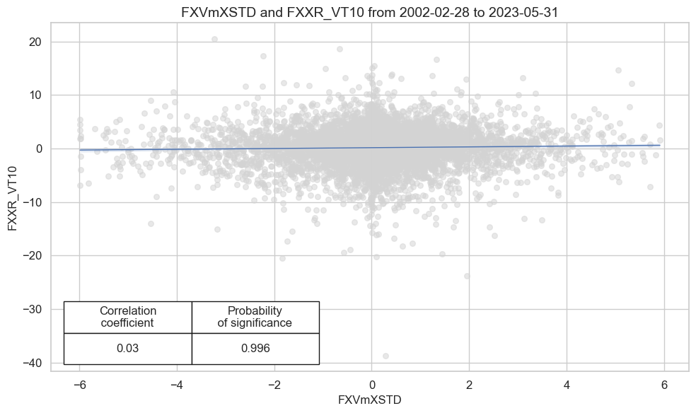
| M: FXVmXSTD/last => FXXR_VT10 | 0.525 | 0.520 | 0.566 | 0.546 | 0.563 | 0.477 | 0.030 | 0.016 | 0.030 | 0.000 | 0.520 |
| Mean cids | 0.527 | 0.517 | 0.568 | 0.547 | 0.560 | 0.474 | 0.018 | 0.506 | 0.021 | 0.536 | 0.516 |
| Mean years | 0.526 | 0.508 | 0.567 | 0.546 | 0.550 | 0.466 | -0.009 | 0.592 | 0.005 | 0.476 | 0.506 |
| Positive ratio | 0.773 | 0.636 | 0.773 | 0.682 | 0.727 | 0.273 | 0.455 | 0.136 | 0.545 | 0.318 | 0.636 |
| Positive ratio | 0.741 | 0.667 | 0.852 | 0.852 | 0.889 | 0.185 | 0.593 | 0.333 | 0.704 | 0.222 | 0.667 |
dix = dict_xsmod
srrx = dix["srr"]
display(srrx.signals_table().sort_index().astype("float").round(3))
| accuracy | bal_accuracy | pos_sigr | pos_retr | pos_prec | neg_prec | pearson | pearson_pval | kendall | kendall_pval | auc | ||||
|---|---|---|---|---|---|---|---|---|---|---|---|---|---|---|
| Return | Signal | Frequency | Aggregation | |||||||||||
| FXXR_VT10 | FXVTREND_Z3 | M | last | 0.525 | 0.52 | 0.566 | 0.546 | 0.563 | 0.477 | 0.021 | 0.091 | 0.028 | 0.001 | 0.52 |
| FXVmXSD | M | last | 0.525 | 0.52 | 0.566 | 0.546 | 0.563 | 0.477 | 0.029 | 0.020 | 0.030 | 0.000 | 0.52 | |
| FXVmXST | M | last | 0.525 | 0.52 | 0.566 | 0.546 | 0.563 | 0.477 | 0.024 | 0.059 | 0.027 | 0.001 | 0.52 | |
| FXVmXSTD | M | last | 0.525 | 0.52 | 0.566 | 0.546 | 0.563 | 0.477 | 0.030 | 0.016 | 0.030 | 0.000 | 0.52 |
Naive PnL #
dix = dict_xsmod

sigx = [dix["sig"]] + dix["rivs"]
targ = dix["targ"]
cidx = dix["cidx"]
blax = dix["black"]

naive_pnl = msn.NaivePnL(
    dfx,
    ret=targ,
    sigs=sigx,
    cids=cidx,
    start="2002-01-01",
    blacklist=blax,
    bms=["USD_EQXR_NSA", "EUR_FXXR_NSA"],
)

for sig in sigx:
    naive_pnl.make_pnl(
        sig,
        sig_neg=False,
        sig_op="zn_score_pan",
        thresh=2,
        rebal_freq="monthly",
        vol_scale=10,
        rebal_slip=1,
        pnl_name=sig + "_PZN",
    )

dix["pnls"] = naive_pnl
As before, we plot two PnL series: the unmodified FX-forward PnL “FXVTREND_Z3_PZN” and modified with external balance dynamics PnL
FXVmXSTD_PZN
. The naïve PnL comparison shows that modification prevented most of the losses that trend following incurred in the 2010s, lifting the long-term Sharpe to 0.3 from 0.2.
dix = dict_xsmod

sigx = ["FXVTREND_Z3"] + [dix["sig"]]
naive_pnl = dix["pnls"]
pnls = [sig + "_PZN" for sig in sigx]
dict_labels = {"FXVTREND_Z3_PZN": "Standard 50-day versus 200 day trend score", "FXVmXSTD_PZN": "modified by external balance dynamics score"}


naive_pnl.plot_pnls(
    pnl_cats=pnls,
    pnl_cids=["ALL"],
    start="2002-01-01",
    title="FX forward PnL (all DM and EM versus USD or EUR) based on simple and modified trend scores",
    xcat_labels=dict_labels,
    figsize=(16, 8),
)
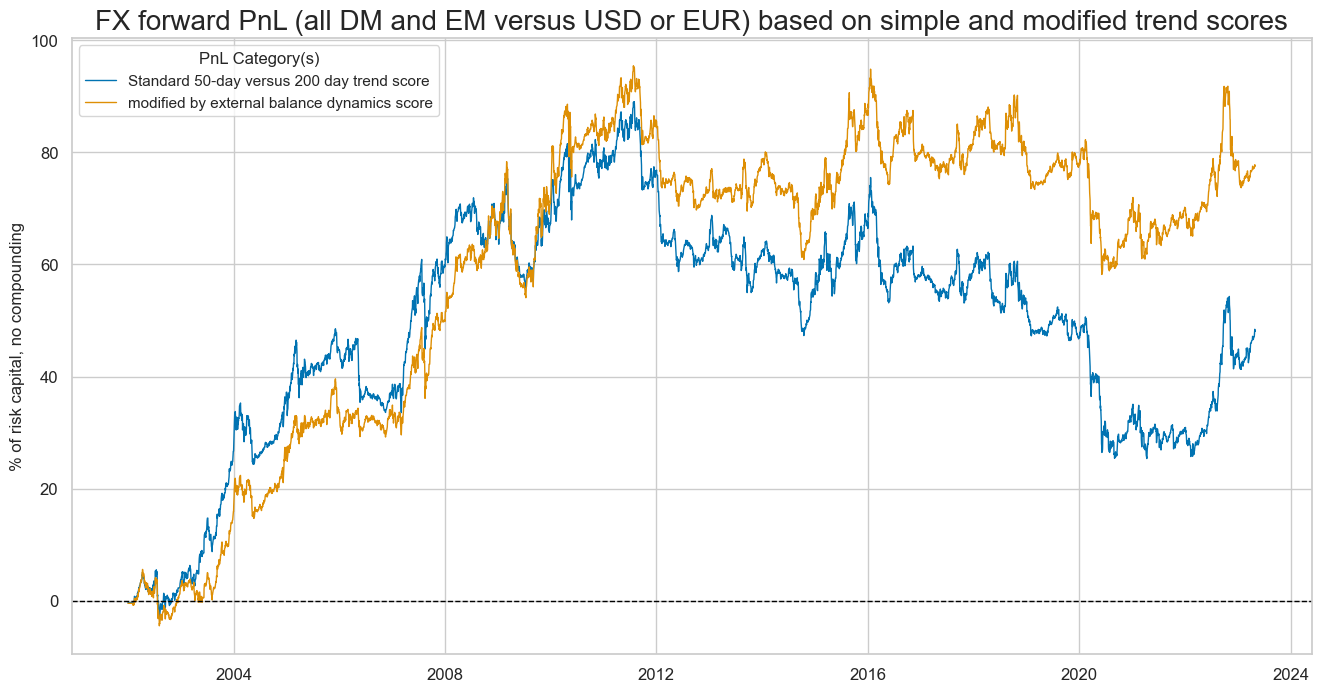
The economic benefit of using the modified trend compared with the simple trend is notable if only since 2012, the modification prevented most of the losses that the trend following incurred in the 2010s, lifting the long-term Sharpe to 0.3 from 0.2.
dix = dict_xsmod

sigx = [dix["sig"]] + dix["rivs"]
naive_pnl = dix["pnls"]
pnls = [sig + "_PZN" for sig in sigx]

df_eval = naive_pnl.evaluate_pnls(
    pnl_cats=pnls,
    pnl_cids=["ALL"],
    start="2002-01-01",
)
display(df_eval.transpose())
| Return % | St. Dev. % | Sharpe Ratio | Sortino Ratio | Max 21-Day Draw % | Max 6-Month Draw % | Peak to Trough Draw % | Top 5% Monthly PnL Share | USD_EQXR_NSA correl | EUR_FXXR_NSA correl | Traded Months | |
|---|---|---|---|---|---|---|---|---|---|---|---|
| xcat | |||||||||||
| FXVmXSTD_PZN | 3.635593 | 10.0 | 0.363559 | 0.503114 | -16.037556 | -22.364889 | -37.208712 | 1.146488 | -0.00448 | 0.011001 | 257 |
| FXVmXSD_PZN | 3.487425 | 10.0 | 0.348743 | 0.48192 | -16.814375 | -20.754997 | -34.178285 | 1.180497 | 0.005503 | 0.019554 | 257 |
| FXVmXST_PZN | 3.044631 | 10.0 | 0.304463 | 0.417349 | -14.883291 | -22.909503 | -47.517242 | 1.31062 | -0.011082 | 0.016872 | 257 |
| FXVTREND_Z3_PZN | 2.254828 | 10.0 | 0.225483 | 0.305464 | -14.177166 | -23.03066 | -63.655385 | 1.717695 | 0.010921 | 0.047578 | 257 |
Balanced trend following #
Specs and panel test #
The alternative to a modified trend is a balanced trend. We use
FXVbXSTD
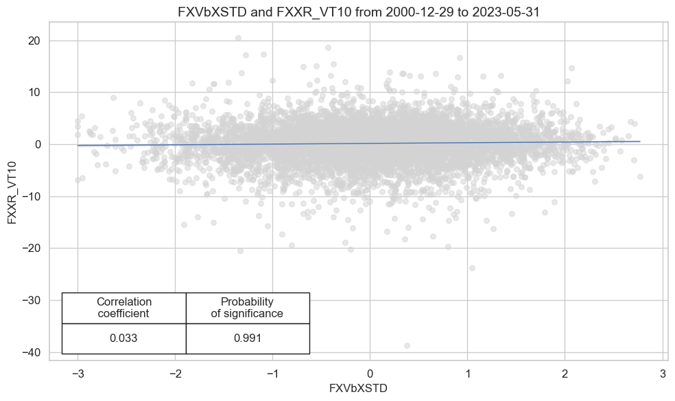
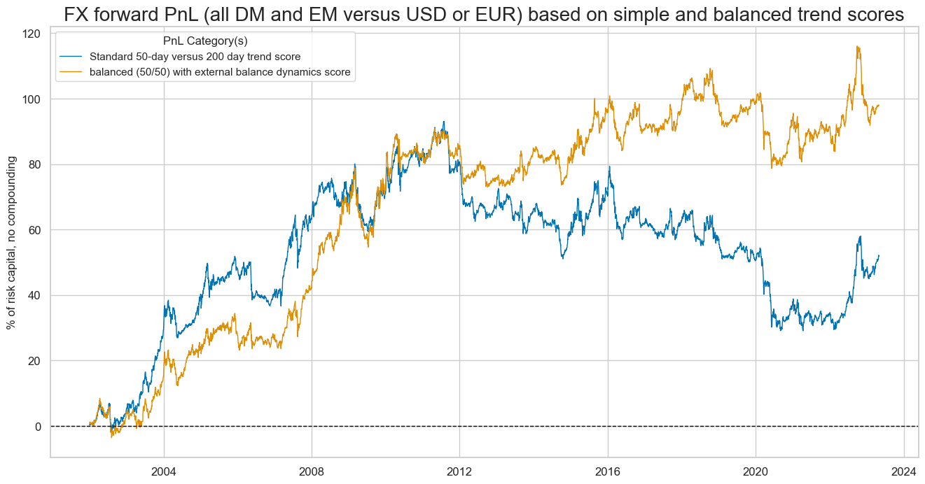
indicator, the average of the trend z-score and the external balance dynamics z-score. The effect of doing so would have been similar to trend modification, albeit a little more pronounced.
sigs = [tr for tr in trendz_bal if tr.startswith("FXV")] + ["FXVTREND_Z3"]
ms = "FXVbXSTD"  # main signal
oths = list(set(sigs) - set([ms]))  # other signals

targ = "FXXR_VT10"
cidx = cids_fx

dict_xsbal = {
    "sig": ms,
    "rivs": oths,
    "targ": targ,
    "cidx": cidx,
    "black": fxblack,
    "srr": None,
    "pnls": None,
}
dix = dict_xsbal

sig = dix["sig"]
targ = dix["targ"]
cidx = dix["cidx"]
blax = dix["black"]

crx = msp.CategoryRelations(
    dfx,
    xcats=[sig, targ],
    cids=cidx,
    freq="M",
    lag=1,
    slip=1,
    xcat_aggs=["last", "sum"],
    start="2000-01-01",
    blacklist=blax,
    xcat_trims=[None, None],
)
crx.reg_scatter(
    labels=False,
    coef_box="lower left",
    # separator=2010,
    xlab=None,
    ylab=None,
    title=None,
    size=(10, 6),
    prob_est="map",
)
Accuracy and correlation bars #
dix = dict_xsbal

sig = dix["sig"]
rivs = dix["rivs"]
targ = dix["targ"]
cidx = dix["cidx"]
blax = dix["black"]

srr = mss.SignalReturnRelations(
    dfx,
    cids=cidx,
    sigs=[sig] + rivs,
    rets=targ,
    freqs="M",
    start="2000-01-01",
    blacklist=blax,
)

dix["srr"] = srr
dix = dict_xsbal
srrx = dix["srr"]
display(srrx.summary_table().sort_index().astype("float").round(3))
| accuracy | bal_accuracy | pos_sigr | pos_retr | pos_prec | neg_prec | pearson | pearson_pval | kendall | kendall_pval | auc | |
|---|---|---|---|---|---|---|---|---|---|---|---|
| M: FXVbXSTD/last => FXXR_VT10 | 0.519 | 0.516 | 0.526 | 0.545 | 0.561 | 0.472 | 0.035 | 0.004 | 0.029 | 0.000 | 0.516 |
| Mean cids | 0.519 | 0.516 | 0.524 | 0.547 | 0.562 | 0.469 | 0.028 | 0.497 | 0.021 | 0.471 | 0.516 |
| Mean years | 0.518 | 0.505 | 0.519 | 0.544 | 0.548 | 0.462 | 0.001 | 0.648 | 0.006 | 0.581 | 0.505 |
| Positive ratio | 0.625 | 0.625 | 0.500 | 0.667 | 0.750 | 0.333 | 0.500 | 0.125 | 0.625 | 0.250 | 0.625 |
| Positive ratio | 0.778 | 0.667 | 0.593 | 0.852 | 0.852 | 0.296 | 0.667 | 0.370 | 0.667 | 0.296 | 0.667 |
Interestingly, balancing the trend signal would have reduced monthly accuracy and balanced accuracy of return predictions relative to simple trend following but significantly increased economic trading value as seen on the plot below.
dix = dict_xsbal
srrx = dix["srr"]
display(srrx.signals_table().sort_index().astype("float").round(3))
| accuracy | bal_accuracy | pos_sigr | pos_retr | pos_prec | neg_prec | pearson | pearson_pval | kendall | kendall_pval | auc | ||||
|---|---|---|---|---|---|---|---|---|---|---|---|---|---|---|
| Return | Signal | Frequency | Aggregation | |||||||||||
| FXXR_VT10 | FXVTREND_Z3 | M | last | 0.528 | 0.523 | 0.558 | 0.545 | 0.565 | 0.480 | 0.024 | 0.048 | 0.032 | 0.000 | 0.523 |
| FXVbXSD | M | last | 0.517 | 0.515 | 0.527 | 0.545 | 0.559 | 0.470 | 0.036 | 0.003 | 0.030 | 0.000 | 0.515 | |
| FXVbXST | M | last | 0.519 | 0.516 | 0.534 | 0.545 | 0.560 | 0.472 | 0.028 | 0.022 | 0.023 | 0.004 | 0.516 | |
| FXVbXSTD | M | last | 0.519 | 0.516 | 0.526 | 0.545 | 0.561 | 0.472 | 0.035 | 0.004 | 0.029 | 0.000 | 0.516 |
Naive PnL #
dix = dict_xsbal

sigx = [dix["sig"]] + dix["rivs"]
targ = dix["targ"]
cidx = dix["cidx"]
blax = dix["black"]

naive_pnl = msn.NaivePnL(
    dfx,
    ret=targ,
    sigs=sigx,
    cids=cidx,
    start="2000-01-01",
    blacklist=blax,
    bms=["USD_EQXR_NSA"],
)

for sig in sigx:
    naive_pnl.make_pnl(
        sig,
        sig_neg=False,
        sig_op="zn_score_pan",
        thresh=2,
        rebal_freq="monthly",
        vol_scale=10,
        rebal_slip=1,
        pnl_name=sig + "_PZN",
    )

dix["pnls"] = naive_pnl
dix = dict_xsbal

sigx = ["FXVTREND_Z3"] + [dix["sig"]]
naive_pnl = dix["pnls"]
pnls = [sig + "_PZN" for sig in sigx]
pnls
['FXVTREND_Z3_PZN', 'FXVbXSTD_PZN']
dix = dict_xsbal

sigx = ["FXVTREND_Z3"] + [dix["sig"]]
naive_pnl = dix["pnls"]
pnls = [sig + "_PZN" for sig in sigx]

dict_labels = {"FXVTREND_Z3_PZN": "Standard 50-day versus 200 day trend score", "FXVbXSTD_PZN": "balanced (50/50) with external balance dynamics score"}


naive_pnl.plot_pnls(
    pnl_cats=pnls,
    pnl_cids=["ALL"],
    start="2002-01-01",
    title="FX forward PnL (all DM and EM versus USD or EUR) based on simple and balanced trend scores",
    xcat_labels=dict_labels,
    figsize=(16, 8),
)
dix = dict_xsbal

sigx = [dix["sig"]] + dix["rivs"]
naive_pnl = dix["pnls"]
pnls = [sig + "_PZN" for sig in sigx]

df_eval = naive_pnl.evaluate_pnls(
    pnl_cats=pnls,
    pnl_cids=["ALL"],
    start="2000-01-01",
)
display(df_eval.transpose())
| Return % | St. Dev. % | Sharpe Ratio | Sortino Ratio | Max 21-Day Draw % | Max 6-Month Draw % | Peak to Trough Draw % | Top 5% Monthly PnL Share | USD_EQXR_NSA correl | Traded Months | |
|---|---|---|---|---|---|---|---|---|---|---|
| xcat | ||||||||||
| FXVbXSTD_PZN | 4.450769 | 10.0 | 0.445077 | 0.623468 | -15.213939 | -21.432764 | -30.578709 | 0.979646 | -0.024611 | 272 |
| FXVTREND_Z3_PZN | 2.82485 | 10.0 | 0.282485 | 0.383203 | -14.392438 | -23.085214 | -64.023928 | 1.412528 | 0.00835 | 272 |
| FXVbXSD_PZN | 4.382106 | 10.0 | 0.438211 | 0.614133 | -16.868248 | -20.543604 | -25.826574 | 1.002185 | -0.016579 | 272 |
| FXVbXST_PZN | 3.774917 | 10.0 | 0.377492 | 0.522907 | -14.866677 | -24.968748 | -41.380084 | 1.1322 | -0.026045 | 272 |
Macro balancing has been essential for trend-following in emerging market currencies. This is plausible since external deficits more often contribute to disruptions of capital flows in the EM space.
dix = dict_xsbal

sigx = [dix["sig"]] + dix["rivs"]
targ = dix["targ"]
cidx = cids_emfx  # focus on EM alone
blax = dix["black"]

naive_pnl = msn.NaivePnL(
    dfx,
    ret=targ,
    sigs=sigx,
    cids=cidx,
    start="2002-01-01",
    blacklist=blax,
    bms=["USD_EQXR_NSA"],
)

for sig in sigx:
    naive_pnl.make_pnl(
        sig,
        sig_neg=False,
        sig_op="zn_score_pan",
        thresh=2,
        rebal_freq="monthly",
        vol_scale=10,
        rebal_slip=1,
        pnl_name=sig + "_PZN",
    )

dix["epnls"] = naive_pnl
dix = dict_xsbal

sigx = ["FXVTREND_Z3"] + [dix["sig"]]
naive_pnl = dix["epnls"]
pnls = [sig + "_PZN" for sig in sigx]
dict_labels={"FXVTREND_Z3_PZN": "Standard 50-day versus 200 day trend score", "FXVbXSTD_PZN": "balanced (50/50) with external balance dynamics score"}


naive_pnl.plot_pnls(
    pnl_cats=pnls,
    pnl_cids=["ALL"],
    start="2002-01-01",
    title="FX forward PnL (EM currencies) based on simple and balanced trend scores",
    xcat_labels=dict_labels,
    figsize=(16, 8),
)
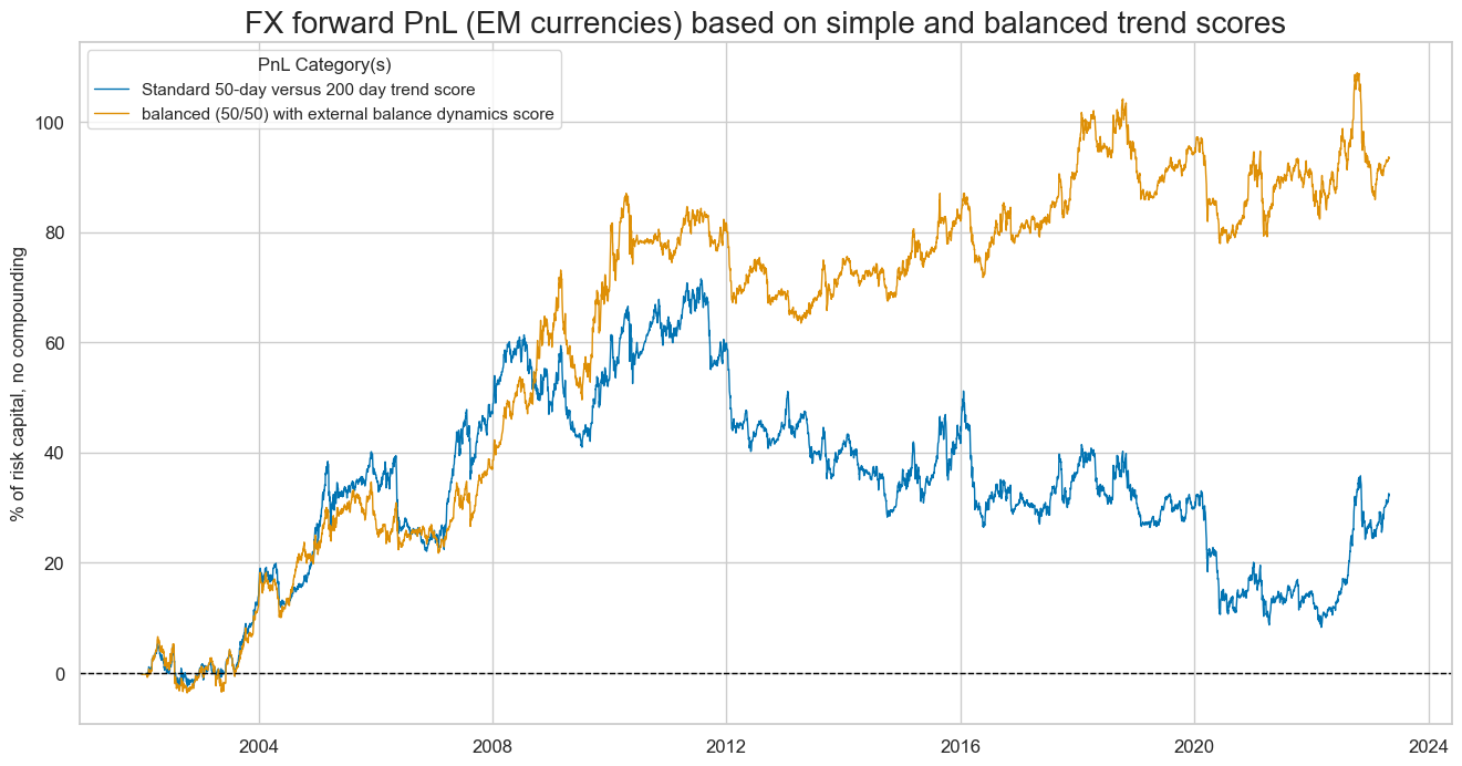
Simple trend following hardly produced any value over the last 20 years in directional EM trading, while balanced trend following at least held on to its boom-time gains during the 2010s and early 2020s.
Relative balanced trend following #
In this section, we investigate the performance of the relative values for original, modified, and balanced trend score signals. “Relative” means that the original value is compared to a basket average. By default, the basket consists of all available cross-sections. We also consider separately emerging markets.
Specs and panel test #
Here we use the relative value trend
FXVTREND_Z3vGFX
as the main signal.
sigs = [tr + "vGFX" for tr in trendz_bal if tr.startswith("FXV")] + ["FXVTREND_Z3vGFX"]
ms = "FXVbXSTDvGFX"  # main signal
oths = list(set(sigs) - set([ms]))  # other signals

targ = "FXXR_VT10vGFX"
cidx = cids_fx

dict_xsbar = {
    "sig": ms,
    "rivs": oths,
    "targ": targ,
    "cidx": cidx,
    "black": fxblack,
    "srr": None,
    "pnls": None,
}
dix = dict_xsbar

sig = dix["sig"]
targ = dix["targ"]
cidx = dix["cidx"]
blax = dix["black"]

crx = msp.CategoryRelations(
    dfx,
    xcats=[sig, targ],
    cids=cidx,
    freq="M",
    lag=1,
    slip=1,
    xcat_aggs=["last", "sum"],
    start="2002-01-01",
    blacklist=blax,
    xcat_trims=[None, None],
)
crx.reg_scatter(
    labels=False,
    coef_box="lower left",
    # separator=2010,
    xlab=None,
    ylab=None,
    title=None,
    size=(10, 6),
    prob_est="map",
)
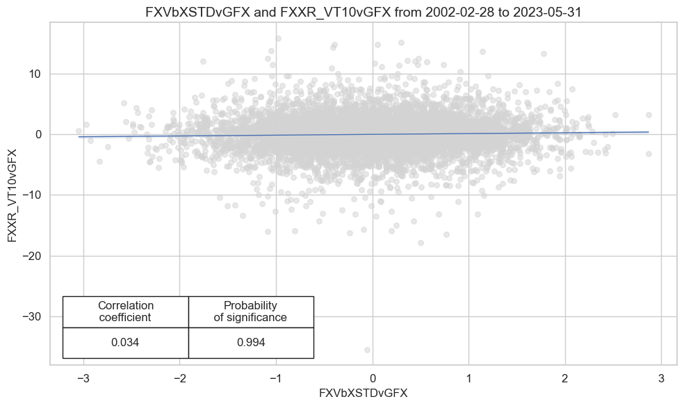
Accuracy and correlation bars #
dix = dict_xsbar

sig = dix["sig"]
rivs = dix["rivs"]
targ = dix["targ"]
cidx = dix["cidx"]
blax = dix["black"]

srr = mss.SignalReturnRelations(
    dfx,
    cids=cidx,
    sigs=[sig] + rivs,
    rets=targ,
    freqs="M",
    start="2002-01-01",
    blacklist=blax,
)

dix["srr"] = srr
dix = dict_xsbar
srrx = dix["srr"]
display(srrx.summary_table().sort_index().astype("float").round(3))
| accuracy | bal_accuracy | pos_sigr | pos_retr | pos_prec | neg_prec | pearson | pearson_pval | kendall | kendall_pval | auc | |
|---|---|---|---|---|---|---|---|---|---|---|---|
| M: FXVbXSTDvGFX/last => FXXR_VT10vGFX | 0.520 | 0.520 | 0.505 | 0.508 | 0.528 | 0.512 | 0.035 | 0.005 | 0.027 | 0.001 | 0.520 |
| Mean cids | 0.521 | 0.519 | 0.504 | 0.510 | 0.528 | 0.510 | 0.031 | 0.444 | 0.019 | 0.418 | 0.519 |
| Mean years | 0.522 | 0.522 | 0.505 | 0.509 | 0.530 | 0.514 | 0.034 | 0.478 | 0.029 | 0.403 | 0.522 |
| Positive ratio | 0.773 | 0.773 | 0.591 | 0.636 | 0.682 | 0.636 | 0.773 | 0.455 | 0.773 | 0.591 | 0.773 |
| Positive ratio | 0.741 | 0.704 | 0.444 | 0.630 | 0.667 | 0.519 | 0.778 | 0.407 | 0.704 | 0.370 | 0.704 |
dix = dict_xsbar
srrx = dix["srr"]
display(srrx.signals_table().sort_index().astype("float").round(3))
| accuracy | bal_accuracy | pos_sigr | pos_retr | pos_prec | neg_prec | pearson | pearson_pval | kendall | kendall_pval | auc | ||||
|---|---|---|---|---|---|---|---|---|---|---|---|---|---|---|
| Return | Signal | Frequency | Aggregation | |||||||||||
| FXXR_VT10vGFX | FXVTREND_Z3vGFX | M | last | 0.513 | 0.513 | 0.496 | 0.508 | 0.521 | 0.505 | 0.035 | 0.006 | 0.026 | 0.002 | 0.513 |
| FXVbXSDvGFX | M | last | 0.514 | 0.514 | 0.501 | 0.508 | 0.522 | 0.506 | 0.037 | 0.003 | 0.026 | 0.002 | 0.514 | |
| FXVbXSTDvGFX | M | last | 0.520 | 0.520 | 0.505 | 0.508 | 0.528 | 0.512 | 0.035 | 0.005 | 0.027 | 0.001 | 0.520 | |
| FXVbXSTvGFX | M | last | 0.515 | 0.515 | 0.499 | 0.508 | 0.523 | 0.507 | 0.028 | 0.028 | 0.022 | 0.008 | 0.515 |
Naive PnL #
dix = dict_xsbar

sigx = [dix["sig"]] + dix["rivs"]
targ = dix["targ"]
cidx = dix["cidx"]
blax = dix["black"]

naive_pnl = msn.NaivePnL(
    dfx,
    ret=targ,
    sigs=sigx,
    cids=cidx,
    start="2002-01-01",
    blacklist=blax,
    bms=["USD_EQXR_NSA"],
)

for sig in sigx:
    naive_pnl.make_pnl(
        sig,
        sig_neg=False,
        sig_op="zn_score_pan",
        thresh=2,
        rebal_freq="monthly",
        vol_scale=10,
        rebal_slip=1,
        pnl_name=sig + "_PZN",
    )

dix["pnls"] = naive_pnl
dix = dict_xsbar

sigx = ["FXVTREND_Z3vGFX"] + [dix["sig"]]
naive_pnl = dix["pnls"]
pnls = [sig + "_PZN" for sig in sigx]

dict_labels={"FXVTREND_Z3vGFX_PZN": "Standard 50-day versus 200 day relative trend score", "FXVbXSTDvGFX_PZN": "balanced (50/50) with relative external balance dynamics score"}


naive_pnl.plot_pnls(
    pnl_cats=pnls,
    pnl_cids=["ALL"],
    start="2002-01-01",
    title="FX forward PnL (all DM/EM relative to basket) based on simple and balanced trend scores",
    xcat_labels=dict_labels,
    figsize=(16, 8),
)
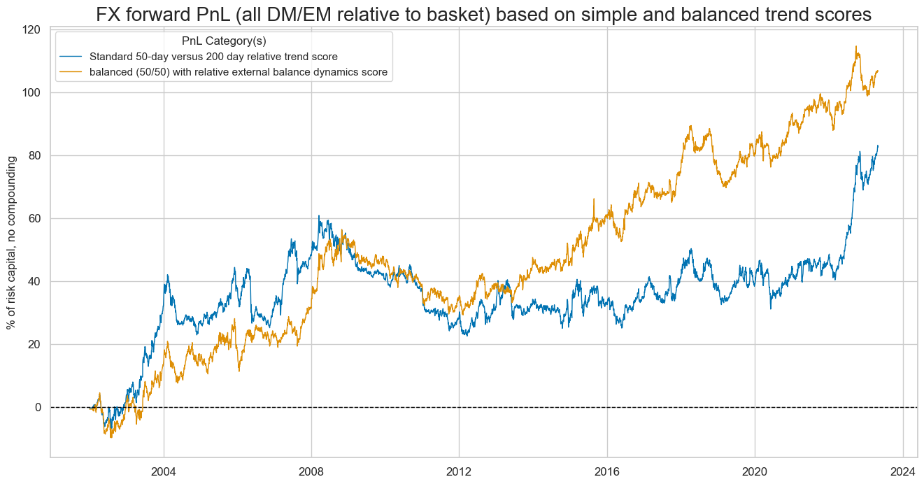
A balanced trend following strategy would have produced a higher naïve PnL value with less seasonality when applied to relative FX forward positions, i.e., trends and returns of any of 27 currencies versus a basket of all currencies. A balanced trend score would have delivered a Sharpe ratio of roughly 0.37.
dix = dict_xsbar

sigx = [dix["sig"]] + dix["rivs"]
naive_pnl = dix["pnls"]
pnls = [sig + "_PZN" for sig in sigx]

df_eval = naive_pnl.evaluate_pnls(
    pnl_cats=pnls,
    pnl_cids=["ALL"],
    start="2000-01-01",
)
display(df_eval.transpose())
| Return % | St. Dev. % | Sharpe Ratio | Sortino Ratio | Max 21-Day Draw % | Max 6-Month Draw % | Peak to Trough Draw % | Top 5% Monthly PnL Share | USD_EQXR_NSA correl | Traded Months | |
|---|---|---|---|---|---|---|---|---|---|---|
| xcat | ||||||||||
| FXVbXSTDvGFX_PZN | 4.999212 | 10.0 | 0.499921 | 0.717658 | -11.3507 | -17.881297 | -27.176256 | 0.78667 | -0.019689 | 257 |
| FXVTREND_Z3vGFX_PZN | 3.868014 | 10.0 | 0.386801 | 0.54129 | -16.879848 | -17.606379 | -38.354457 | 1.133795 | -0.004897 | 257 |
| FXVbXSTvGFX_PZN | 4.10675 | 10.0 | 0.410675 | 0.589219 | -13.179912 | -16.692129 | -33.57859 | 1.045019 | -0.012644 | 257 |
| FXVbXSDvGFX_PZN | 5.146542 | 10.0 | 0.514654 | 0.740068 | -11.898182 | -17.489869 | -23.562371 | 0.751389 | -0.020975 | 257 |
Relative balanced EM trend following #
The post argues, that macro balancing particularly in the context of trend-following in emerging market (EM) currencies, has been considered crucial. This is due to the fact that external deficits tend to play a significant role in causing disruptions to capital flows in the EM space. Simple trend following strategies have generally not been as effective in generating substantial returns in directional EM trading over the past two decades. However, balanced trend following approaches have demonstrated the ability to preserve gains made during periods of market booms, specifically in the 2010s and early 2020s.
Specs and panel test #
Here we use the relative indicator
FXVbXSTDvEFX
created earlier as relative to emerging markets currencies basket
sigs = [tr + "vEFX" for tr in trendz_bal if tr.startswith("FXV")] + ["FXVTREND_Z3vEFX"]
ms = "FXVbXSTDvEFX"  # main signal
oths = list(set(sigs) - set([ms]))  # other signals

targ = "FXXR_VT10vEFX"
cidx = cids_emfx

dict_xsbae = {
    "sig": ms,
    "rivs": oths,
    "targ": targ,
    "cidx": cidx,
    "black": fxblack,
    "srr": None,
    "pnls": None,
}
dix = dict_xsbae

sig = dix["sig"]
targ = dix["targ"]
cidx = dix["cidx"]
blax = dix["black"]

crx = msp.CategoryRelations(
    dfx,
    xcats=[sig, targ],
    cids=cidx,
    freq="M",
    lag=1,
    slip=1,
    xcat_aggs=["last", "sum"],
    start="2000-01-01",
    blacklist=blax,
    xcat_trims=[None, None],
)
crx.reg_scatter(
    labels=False,
    coef_box="lower left",
    # separator=2010,
    xlab=None,
    ylab=None,
    title=None,
    size=(10, 6),
    prob_est="map",
)
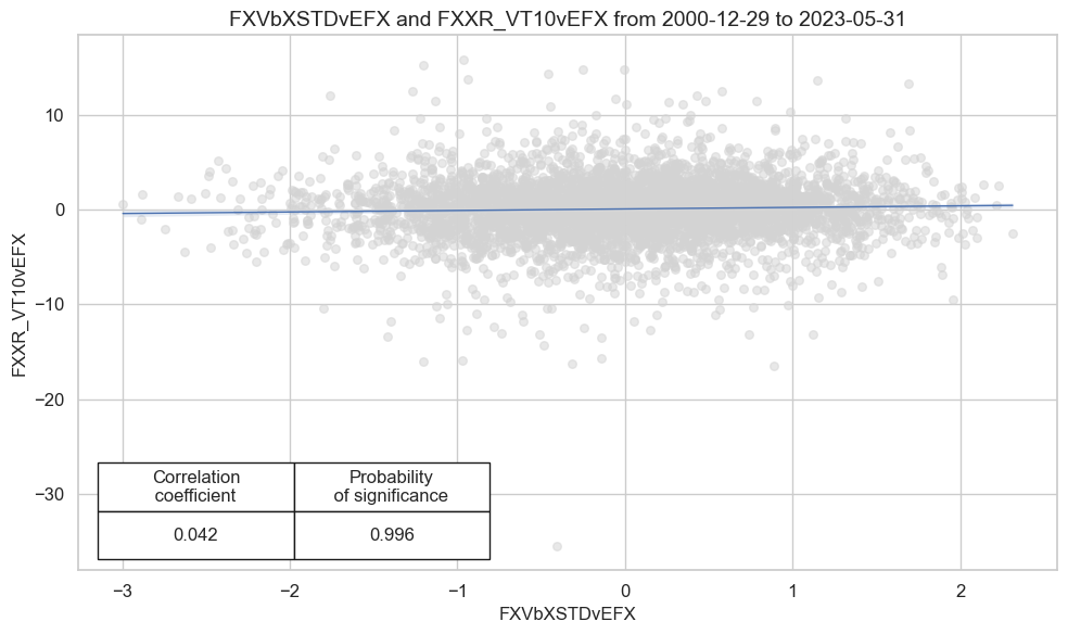
Accuracy and correlation bars #
dix = dict_xsbae

sig = dix["sig"]
rivs = dix["rivs"]
targ = dix["targ"]
cidx = dix["cidx"]
blax = dix["black"]

srr = mss.SignalReturnRelations(
    dfx,
    cids=cidx,
    sigs=[sig] + rivs,
    rets=targ,
    freqs="M",
    start="2002-01-01",
    blacklist=blax,
)

dix["srr"] = srr
dix = dict_xsbae
srrx = dix["srr"]
display(srrx.summary_table().sort_index().astype("float").round(3))
| accuracy | bal_accuracy | pos_sigr | pos_retr | pos_prec | neg_prec | pearson | pearson_pval | kendall | kendall_pval | auc | |
|---|---|---|---|---|---|---|---|---|---|---|---|
| M: FXVbXSTDvEFX/last => FXXR_VT10vEFX | 0.525 | 0.524 | 0.509 | 0.527 | 0.551 | 0.497 | 0.049 | 0.001 | 0.037 | 0.000 | 0.524 |
| Mean cids | 0.525 | 0.525 | 0.505 | 0.529 | 0.555 | 0.496 | 0.053 | 0.447 | 0.035 | 0.404 | 0.525 |
| Mean years | 0.526 | 0.526 | 0.507 | 0.530 | 0.554 | 0.497 | 0.049 | 0.420 | 0.038 | 0.377 | 0.526 |
| Positive ratio | 0.818 | 0.818 | 0.545 | 0.727 | 0.818 | 0.500 | 0.818 | 0.545 | 0.818 | 0.636 | 0.818 |
| Positive ratio | 0.842 | 0.842 | 0.526 | 0.842 | 0.842 | 0.421 | 0.895 | 0.526 | 0.895 | 0.474 | 0.842 |
dix = dict_xsbae
srrx = dix["srr"]
display(srrx.signals_table().sort_index().astype("float").round(3))
| accuracy | bal_accuracy | pos_sigr | pos_retr | pos_prec | neg_prec | pearson | pearson_pval | kendall | kendall_pval | auc | ||||
|---|---|---|---|---|---|---|---|---|---|---|---|---|---|---|
| Return | Signal | Frequency | Aggregation | |||||||||||
| FXXR_VT10vEFX | FXVTREND_Z3vEFX | M | last | 0.516 | 0.515 | 0.507 | 0.527 | 0.542 | 0.488 | 0.036 | 0.018 | 0.030 | 0.003 | 0.515 |
| FXVbXSDvEFX | M | last | 0.520 | 0.520 | 0.502 | 0.527 | 0.547 | 0.493 | 0.055 | 0.000 | 0.040 | 0.000 | 0.520 | |
| FXVbXSTDvEFX | M | last | 0.525 | 0.524 | 0.509 | 0.527 | 0.551 | 0.497 | 0.049 | 0.001 | 0.037 | 0.000 | 0.524 | |
| FXVbXSTvEFX | M | last | 0.515 | 0.515 | 0.508 | 0.527 | 0.542 | 0.488 | 0.031 | 0.038 | 0.025 | 0.013 | 0.515 |
Naive PnL #
dix = dict_xsbae

sigx = [dix["sig"]] + dix["rivs"]
targ = dix["targ"]
cidx = dix["cidx"]
blax = dix["black"]

naive_pnl = msn.NaivePnL(
    dfx,
    ret=targ,
    sigs=sigx,
    cids=cidx,
    start="2002-01-01",
    blacklist=blax,
    bms=["USD_EQXR_NSA"],
)

for sig in sigx:
    naive_pnl.make_pnl(
        sig,
        sig_neg=False,
        sig_op="zn_score_pan",
        thresh=2,
        rebal_freq="monthly",
        vol_scale=10,
        rebal_slip=1,
        pnl_name=sig + "_PZN",
    )

dix["pnls"] = naive_pnl
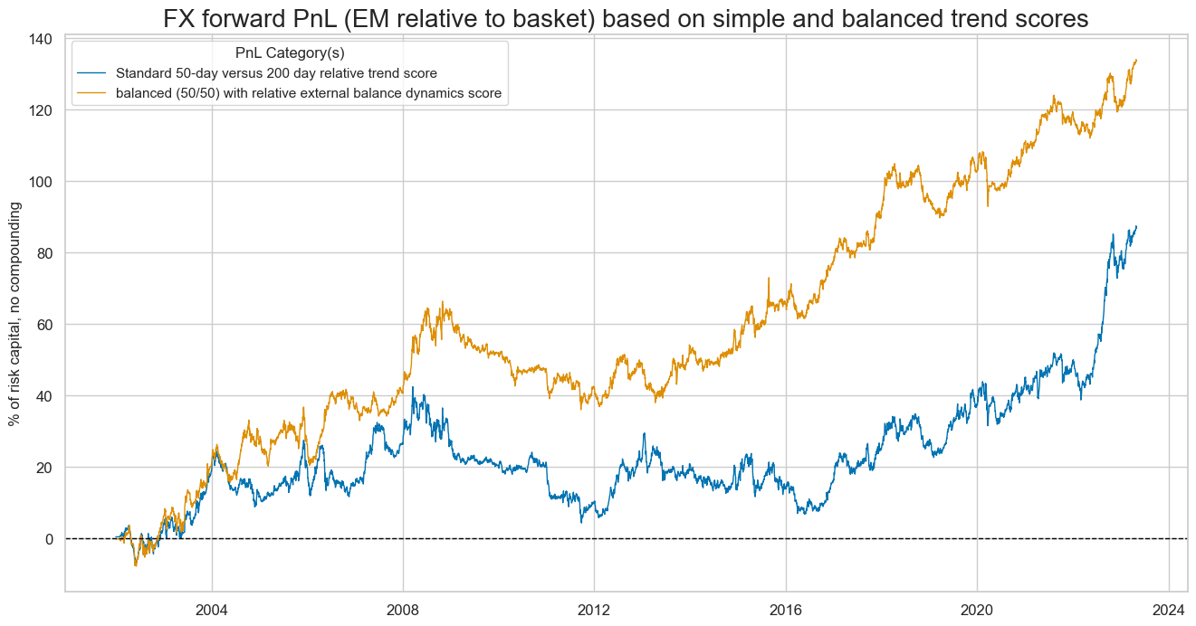
The importance of external balance adjustment has turned out to be greater for the EM space, where a balanced trend score would have produced a long-term naïve Sharpe ratio of 0.48 and more consistent value generation than a simple trend score.
dix = dict_xsbae

sigx = ["FXVTREND_Z3vEFX"] + [dix["sig"]]
naive_pnl = dix["pnls"]
pnls = [sig + "_PZN" for sig in sigx]

dict_labels={"FXVTREND_Z3vEFX_PZN": "Standard 50-day versus 200 day relative trend score", "FXVbXSTDvEFX_PZN": "balanced (50/50) with relative external balance dynamics score"}

naive_pnl.plot_pnls(
    pnl_cats=pnls,
    pnl_cids=["ALL"],
    start="2002-01-01",
    title="FX forward PnL (EM relative to basket) based on simple and balanced trend scores",
    xcat_labels=dict_labels,
    figsize=(16, 8),
)
dix = dict_xsbae

sigx = [dix["sig"]] + dix["rivs"]
naive_pnl = dix["pnls"]
pnls = [sig + "_PZN" for sig in sigx]

df_eval = naive_pnl.evaluate_pnls(
    pnl_cats=pnls,
    pnl_cids=["ALL"],
    start="2000-01-01",
)
display(df_eval.transpose())
| Return % | St. Dev. % | Sharpe Ratio | Sortino Ratio | Max 21-Day Draw % | Max 6-Month Draw % | Peak to Trough Draw % | Top 5% Monthly PnL Share | USD_EQXR_NSA correl | Traded Months | |
|---|---|---|---|---|---|---|---|---|---|---|
| xcat | ||||||||||
| FXVbXSTDvEFX_PZN | 6.262213 | 10.0 | 0.626221 | 0.905232 | -12.896053 | -13.995904 | -30.384818 | 0.685057 | 0.017571 | 257 |
| FXVbXSTvEFX_PZN | 4.067901 | 10.0 | 0.40679 | 0.583447 | -17.437298 | -16.756701 | -45.228387 | 1.138687 | 0.022324 | 257 |
| FXVTREND_Z3vEFX_PZN | 4.071955 | 10.0 | 0.407195 | 0.572564 | -12.496685 | -15.633018 | -38.119727 | 1.089481 | 0.011843 | 257 |
| FXVbXSDvEFX_PZN | 7.067251 | 10.0 | 0.706725 | 1.025476 | -10.427437 | -12.36921 | -25.124515 | 0.602983 | 0.009045 | 257 |