FX signals with ML and common sense #
Get packages and JPMaQS data #
import os
import numpy as np
import pandas as pd

from sklearn.pipeline import Pipeline
from sklearn.linear_model import LinearRegression, ElasticNet
from sklearn.ensemble import RandomForestRegressor

from sklearn.metrics import (
    make_scorer,
    r2_score,
)

import macrosynergy.management as msm
import macrosynergy.panel as msp
import macrosynergy.pnl as msn
import macrosynergy.signal as mss
import macrosynergy.learning as msl
import macrosynergy.visuals as msv

from macrosynergy.download import JPMaQSDownload

import warnings

warnings.simplefilter("ignore")
# Cross-sections of interest - FX
cids_g3 = ["EUR", "USD"]  # DM large currency areas
cids_dmfx = ["AUD", "CAD", "CHF", "GBP", "JPY", "NOK", "NZD", "SEK"]  # 8 DM currency areas
cids_emfx = ["CZK", "ILS", "KRW", "MXN", "PLN", "THB", "TWD", "ZAR"]  # 8 EM currency areas

cids_fx = cids_dmfx + cids_emfx

cids_dm = cids_g3 + cids_dmfx
cids = cids_dm + cids_emfx

cids_eur = ["CHF", "NOK", "SEK", "PLN", "HUF", "CZK"]  # trading against EUR
cids_eud = ["GBP"]  # trading against EUR and USD
cids_usd = list(set(cids_fx) - set(cids_eur + cids_eud))  # trading against USD
# Quantamental categories for factor and target calculations
xbds = [
"MTBGDPRATIO_SA_3MMA_D1M1ML3",
"MTBGDPRATIO_SA_6MMA_D1M1ML6",
"MTBGDPRATIO_NSA_12MMA_D1M1ML3",
"BXBGDPRATIO_NSA_12MMA_D1M1ML3"
]
xbrs = [
"CABGDPRATIO_NSA_12MMA",
"BXBGDPRATIO_NSA_12MMA"
]
pcg = [
"PCREDITBN_SJA_P1M1ML12"
]
ipgs = [
"IP_SA_P6M6ML6AR",
"IP_SA_P1M1ML12_3MMA"
]
ir = [
"RIR_NSA",
]
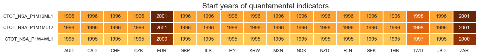
ctots = [
"CTOT_NSA_P1M1ML12",
"CTOT_NSA_P1M12ML1",
"CTOT_NSA_P1W4WL1",
]
surv = [
"MBCSCORE_SA_D3M3ML3",
"MBCSCORE_SA_D1Q1QL1",
"MBCSCORE_SA_D6M6ML6",
"MBCSCORE_SA_D2Q2QL2",
]
ppi = [
"PGDPTECH_SA_P1M1ML12_3MMA",
"PPIH_NSA_P1M1ML12_3MMA"
]
gdps = [
"INTRGDP_NSA_P1M1ML12_3MMA",
"RGDPTECH_SA_P1M1ML12_3MMA",
]
emp = [
"UNEMPLRATE_SA_D3M3ML3",
"UNEMPLRATE_SA_D6M6ML6",
"UNEMPLRATE_SA_D1Q1QL1",
"UNEMPLRATE_SA_D2Q2QL2",
"UNEMPLRATE_NSA_3MMA_D1M1ML12",
"UNEMPLRATE_NSA_D1Q1QL4",
]
iip = [
"IIPLIABGDP_NSA_D1Mv2YMA",
"IIPLIABGDP_NSA_D1Mv5YMA",
]
cpi = [
"CPIC_SA_P1M1ML12",
"CPIC_SJA_P6M6ML6AR",
"CPIH_SA_P1M1ML12",
"CPIH_SJA_P6M6ML6AR",
"INFE1Y_JA",
"INFE2Y_JA",
"INFE5Y_JA",
]
main = xbds + xbrs + pcg + ipgs + ir + ctots + surv + ppi + gdps + emp + iip + cpi
adds = [
"INFTEFF_NSA",
"RGDP_SA_P1Q1QL4_20QMM"
]
mkts = [
"FXTARGETED_NSA",
"FXUNTRADABLE_NSA",
]
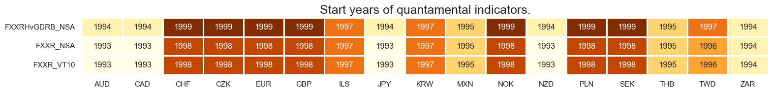
rets = [
"FXXR_NSA",
"FXXR_VT10",
"FXXRHvGDRB_NSA",
]
xcats = main + mkts + rets + adds
# Resultant tickers for download
single_tix = ["USD_GB10YXR_NSA", "EUR_FXXR_NSA", "USD_EQXR_NSA"]
tickers = [cid + "_" + xcat for cid in cids for xcat in xcats] + single_tix
# Download series from J.P. Morgan DataQuery by tickers

start_date = "1990-01-01"
end_date = None

# Retrieve credentials

oauth_id = os.getenv("DQ_CLIENT_ID")  # Replace with own client ID
oauth_secret = os.getenv("DQ_CLIENT_SECRET")  # Replace with own secret

# Download from DataQuery

downloader = JPMaQSDownload(client_id=oauth_id, client_secret=oauth_secret)
df = downloader.download(
    tickers=tickers,
    start_date=start_date,
    end_date=end_date,
    metrics=["value"],
    suppress_warning=True,
    show_progress=True,
)

dfx = df.copy()
dfx.info()
Downloading data from JPMaQS.
Timestamp UTC:  2024-12-20 09:56:12
Connection successful!
Requesting data: 100%|█████████████████████████████████████████████████████████████████| 39/39 [00:08<00:00,  4.83it/s]
Downloading data: 100%|████████████████████████████████████████████████████████████████| 39/39 [00:27<00:00,  1.40it/s]
Some expressions are missing from the downloaded data. Check logger output for complete list.
97 out of 776 expressions are missing. To download the catalogue of all available expressions and filter the unavailable expressions, set `get_catalogue=True` in the call to `JPMaQSDownload.download()`.
Some dates are missing from the downloaded data.
2 out of 9127 dates are missing.
<class 'pandas.core.frame.DataFrame'>
RangeIndex: 5033333 entries, 0 to 5033332
Data columns (total 4 columns):
 #   Column     Dtype
---  ------     -----
 0   real_date  datetime64[ns]
 1   cid        object
 2   xcat       object
 3   value      float64
dtypes: datetime64[ns](1), float64(1), object(2)
memory usage: 153.6+ MB
Availability and blacklisting #
Renaming #
Rename quarterly tickers to roughly equivalent monthly tickers to simplify subsequent operations.
dict_repl = {
    "UNEMPLRATE_NSA_D1Q1QL4": "UNEMPLRATE_NSA_3MMA_D1M1ML12",
    "UNEMPLRATE_SA_D1Q1QL1": "UNEMPLRATE_SA_D3M3ML3",
    "UNEMPLRATE_SA_D2Q2QL2": "UNEMPLRATE_SA_D6M6ML6",
    "MBCSCORE_SA_D1Q1QL1": "MBCSCORE_SA_D3M3ML3",
    "MBCSCORE_SA_D2Q2QL2": "MBCSCORE_SA_D6M6ML6",
}

for key, value in dict_repl.items():
    dfx["xcat"] = dfx["xcat"].str.replace(key, value)
Check availability #
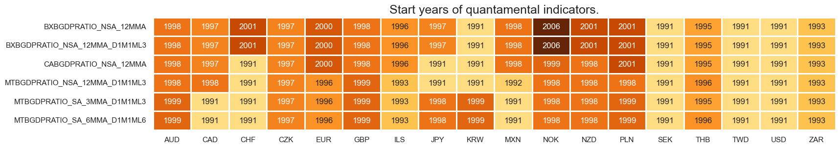
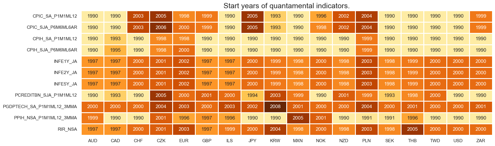
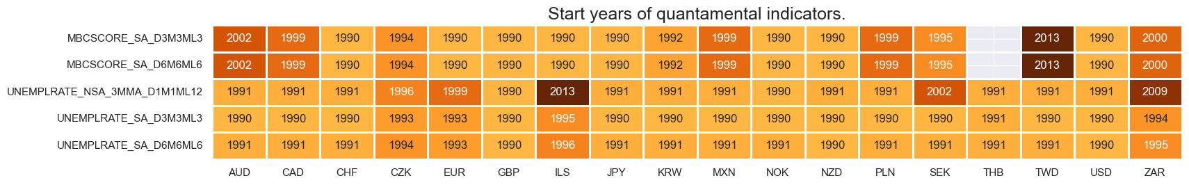
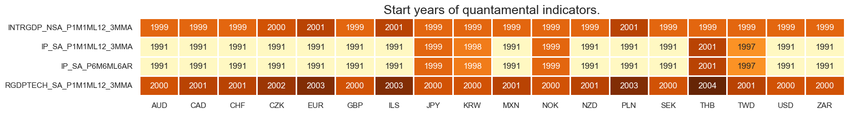
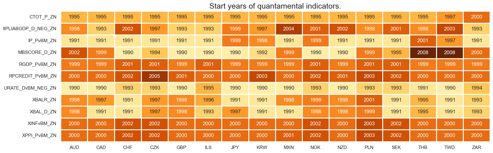
Prior to commencing any analysis, it is crucial to evaluate the accessibility of data. This evaluation serves several purposes, including identifying potential data gaps or constraints within the dataset. Such gaps can significantly influence the trustworthiness and accuracy of the analysis. Moreover, it aids in verifying that ample observations are accessible for each chosen category and cross-section. Additionally, it assists in establishing suitable timeframes for conducting the analysis.
xcatx = xbds + xbrs
msm.check_availability(df=dfx, xcats=xcatx, cids=cids, missing_recent=False)
xcatx = cpi + ppi + ir + pcg
msm.check_availability(df=dfx, xcats=xcatx, cids=cids, missing_recent=False)
xcatx = surv + emp
msm.check_availability(df=dfx, xcats=xcatx, cids=cids, missing_recent=False)
xcatx = gdps + ipgs
msm.check_availability(df=dfx, xcats=xcatx, cids=cids, missing_recent=False)
xcatx = ctots
msm.check_availability(df=dfx, xcats=xcatx, cids=cids, missing_recent=False)
xcatx = iip
msm.check_availability(df=dfx, xcats=xcatx, cids=cids, missing_recent=False)

xcatx = rets
msm.check_availability(df=dfx, xcats=xcatx, cids=cids, missing_recent=False)
Blacklisting #
Identifying and isolating periods of official exchange rate targets, illiquidity, or convertibility-related distortions in FX markets is the first step in creating an FX trading strategy. These periods can significantly impact the behavior and dynamics of currency markets, and failing to account for them can lead to inaccurate or misleading findings. A standard blacklist dictionary (
fxblack
in the cell below) can be passed to several
macrosynergy
package functions that exclude the blacklisted periods from related analyses.
# Create blacklisting dictionary

dfb = df[df["xcat"].isin(["FXTARGETED_NSA", "FXUNTRADABLE_NSA"])].loc[
    :, ["cid", "xcat", "real_date", "value"]
]
dfba = (
    dfb.groupby(["cid", "real_date"])
    .aggregate(value=pd.NamedAgg(column="value", aggfunc="max"))
    .reset_index()
)
dfba["xcat"] = "FXBLACK"
fxblack = msp.make_blacklist(dfba, "FXBLACK")
fxblack
{'CHF': (Timestamp('2011-10-03 00:00:00'), Timestamp('2015-01-30 00:00:00')),
 'CZK': (Timestamp('2014-01-01 00:00:00'), Timestamp('2017-07-31 00:00:00')),
 'ILS': (Timestamp('1999-01-01 00:00:00'), Timestamp('2005-12-30 00:00:00')),
 'THB': (Timestamp('2007-01-01 00:00:00'), Timestamp('2008-11-28 00:00:00'))}
Factor computation and checks #
Single-concept calculations #
# Initiate factor dictionary

factors = {}
International liabilities trends #
# Combine to single trend measure
cidx = cids
xcatx = [
    "IIPLIABGDP_NSA_D1Mv2YMA",
    "IIPLIABGDP_NSA_D1Mv5YMA",
]
xtic = "IIPLIABGDP_D"
label = "International liabilities trend"

dfa = msp.linear_composite(
    dfx,
    xcats=xcatx,
    cids=cidx,
    weights=[1/2, 1/5],
    normalize_weights=True,
    complete_xcats=False,
    new_xcat=xtic,
)

dfx = msm.update_df(dfx, dfa)
factors[xtic] =[label, "ABS", "NEG"]  # info on benchmark/sign adjustments
External balances trends #
# Combine to single trend measure
cidx = cids
xcatx = [
    "MTBGDPRATIO_SA_3MMA_D1M1ML3",
    "MTBGDPRATIO_SA_6MMA_D1M1ML6",
    "BXBGDPRATIO_NSA_12MMA_D1M1ML3"
]
xtic = "XBAL_D"
label = "External balances change"

dfa = msp.linear_composite(
    dfx,
    xcats=xcatx,
    cids=cidx,
    weights=[1, 1/2, 1],
    normalize_weights=True,
    complete_xcats=False,
    new_xcat=xtic,
)

dfx = msm.update_df(dfx, dfa)
factors[xtic] =[label, "ABS", "POS"]  # info on benchmark/sign adjustments
External balances ratios #
# Combine to single ratio
cidx = cids
xcatx = [
    "CABGDPRATIO_NSA_12MMA",
    "BXBGDPRATIO_NSA_12MMA"
]
xtic = "XBALR"
label = "External balances ratios"

dfa = msp.linear_composite(
    dfx,
    xcats=xcatx,
    cids=cidx,
    normalize_weights=True,
    complete_xcats=False,
    new_xcat=xtic,
)

dfx = msm.update_df(dfx, dfa)
factors[xtic] =[label, "ABS", "POS"]  # info on benchmark/sign adjustments
Unemployment rate changes #
# Combine to annualized change average
xcatx = [
    "UNEMPLRATE_SA_D3M3ML3",
    "UNEMPLRATE_SA_D6M6ML6",
    "UNEMPLRATE_NSA_3MMA_D1M1ML12",
]
cidx = cids
xtic = "URATE_D"
label = "Unemployment rate change"

dfa = msp.linear_composite(
    dfx,
    xcats=xcatx,
    cids=cidx,
    weights=[4, 2, 1],
    normalize_weights=True,
    complete_xcats=False,
    new_xcat=xtic,
)

dfx = msm.update_df(dfx, dfa)
factors[xtic] =[label, "REL", "NEG"]  # info on benchmark/sign adjustments
Excess CPI inflation pressure #
cidx = cids
xcatx = [
    "CPIC_SA_P1M1ML12",
    "CPIC_SJA_P6M6ML6AR",
    "CPIH_SA_P1M1ML12",
    "CPIH_SJA_P6M6ML6AR",
    "INFE1Y_JA",
    "INFE2Y_JA",
    "INFE5Y_JA",
]

dfa = msp.linear_composite(
    dfx,
    xcats=xcatx,
    cids=cidx,
    complete_xcats=False,
    new_xcat="INF",
)

dfx = msm.update_df(dfx, dfa)
cidx = cids
xtic = "XINF"
label = "Excess CPI inflation pressure"

calcs = [f"{xtic} = INF - INFTEFF_NSA"]
dfa = msp.panel_calculator(dfx, calcs=calcs, cids=cidx)
dfx = msm.update_df(dfx, dfa)
factors[xtic] =[label, "REL", "POS"]  # info on benchmark/sign adjustments
Excess producer price inflation #
cidx = cids
xcatx = [
    "PGDPTECH_SA_P1M1ML12_3MMA",
    "PPIH_NSA_P1M1ML12_3MMA"
]

dfa = msp.linear_composite(
    dfx,
    xcats=xcatx,
    cids=cidx,
    complete_xcats=False,
    new_xcat="PPI_P",
)

dfx = msm.update_df(dfx, dfa)
cidx = cids
xtic = "XPPI_P"
label = "Excess producer inflation"

calcs = [f"{xtic} = PPI_P - INFTEFF_NSA"]
dfa = msp.panel_calculator(dfx, calcs=calcs, cids=cidx)
dfx = msm.update_df(dfx, dfa)
factors[xtic] =[label, "REL", "POS"]  # info on benchmark/sign adjustments
Real credit growth #
cidx = cids
xtic = "RPCREDIT_P"
label = "Real credit growth"

calcs = [f"{xtic} = PCREDITBN_SJA_P1M1ML12 - INFTEFF_NSA"]
dfa = msp.panel_calculator(dfx, calcs=calcs, cids=cidx)
dfx = msm.update_df(dfx, dfa)
factors[xtic] =[label, "REL", "POS"]  # info on benchmark/sign adjustments
Real GDP growth estimates #
cidx = cids
xcatx = [
    "RGDPTECH_SA_P1M1ML12_3MMA",
    "INTRGDP_NSA_P1M1ML12_3MMA",
]
xtic = "RGDP_P"
label = "Real GDP growth"

dfa = msp.linear_composite(
    dfx,
    xcats=xcatx,
    cids=cidx,
    complete_xcats=False,
    new_xcat=xtic,
)

dfx = msm.update_df(dfx, dfa)
factors[xtic] =[label, "REL", "POS"]  # info on benchmark/sign adjustments
Industrial production growth #
cidx = cids
xcatx = [
    "IP_SA_P6M6ML6AR",
    "IP_SA_P1M1ML12_3MMA"
]
xtic = "IP_P"
label = "Industry growth"

dfa = msp.linear_composite(
    dfx,
    xcats=xcatx,
    cids=cidx,
    complete_xcats=False,
    new_xcat=xtic,
)

dfx = msm.update_df(dfx, dfa)
factors[xtic] =[label, "REL", "POS"]  # info on benchmark/sign adjustments
Manufacturing confidence improvement #
cidx = cids
xcatx = ["MBCSCORE_SA_D3M3ML3", "MBCSCORE_SA_D6M6ML6"]
xtic = "MBSCORE_D"
label = "Manufacturing confidence change"

dfa = msp.linear_composite(
    dfx,
    xcats=xcatx,
    cids=cidx,
    weights=[2, 1],
    normalize_weights=True,
    complete_xcats=False,
    new_xcat=xtic,
)
dfx = msm.update_df(dfx, dfa)
factors[xtic] =[label, "ABS", "POS"]  # info on benchmark/sign adjustments
Commodity-based terms of trade improvement #
cidx = cids
xcatx = ["CTOT_NSA_P1M1ML12", "CTOT_NSA_P1M12ML1", "CTOT_NSA_P1W4WL1"]
xtic = "CTOT_P"
label = "Terms-of-trade change"

dfa = msp.linear_composite(
    dfx,
    xcats=xcatx,
    cids=cidx,
    weights=[1/12, 1/6, 2],
    normalize_weights=True,
    complete_xcats=False,
    new_xcat=xtic,
)
dfx = msm.update_df(dfx, dfa)
factors[xtic] =[label, "ABS", "POS"]  # info on benchmark/sign adjustments
Transformations and visualizations #
Relative values #
# Calculate relative values to benchmark currency areas

xcatx = [f for f in factors.keys() if factors[f][1] == "REL"]

dfa_usd = msp.make_relative_value(dfx, xcatx, cids_usd, basket=["USD"], postfix="vBM")
dfa_eur = msp.make_relative_value(dfx, xcatx, cids_eur, basket=["EUR"], postfix="vBM")
dfa_eud = msp.make_relative_value(
    dfx, xcatx, cids_eud, basket=["EUR", "USD"], postfix="vBM"
)

dfa = pd.concat([dfa_eur, dfa_usd, dfa_eud])
dfx = msm.update_df(dfx, dfa)

# Modified factor dictionary

factors_r = {(f + "vBM" if k[1] == "REL" else f): k for f, k in factors.items()}
Negative values #
# Negative values where required

xcatx = [f for f in factors_r.keys() if factors_r[f][2] == "NEG"]
calcs = []

for xc in xcatx:
    calcs += [f"{xc}_NEG = - {xc}"]

dfa = msp.panel_calculator(dfx, calcs=calcs, cids=cids_fx)
dfx = msm.update_df(dfx, dfa)

# Modified factor dictionary

factors_rn = {(f + "_NEG" if k[2] == "NEG" else f): k for f, k in factors_r.items()}
Normalization #
# Zn-scores

xcatx = [f for f in factors_rn.keys()]
cidx = cids_fx

dfa = pd.DataFrame(columns=list(dfx.columns))

for xc in xcatx:
    dfaa = msp.make_zn_scores(
        dfx,
        xcat=xc,
        cids=cidx,
        sequential=True,
        min_obs=261 * 3,
        neutral="zero",
        pan_weight=1,
        thresh=3,
        postfix="_ZN",
        est_freq="m",
    )
    dfa = msm.update_df(dfa, dfaa)

dfx = msm.update_df(dfx, dfa)

# Modified factor dictionary

factorz = {f + "_ZN": k for f, k in factors_rn.items()}
# Labels dictionary

xtix = [f for f in factorz.keys()]
labs = [
    (
        "Relative " + v[0][:1].lower() + v[0][1:] + ", negative"
        if v[1] == "REL" and v[2] == "NEG"
        else (
            "Relative " + v[0][:1].lower() + v[0][1:]
            if v[1] == "REL" and v[2] == "POS"
            else v[0] + ", negative" if v[2] == "NEG" else v[0]
        )
    )
    for v in factorz.values()
]

factorz_labs = dict(zip(xtix, labs))
Visual checks #
cidx = cids_fx
xcatx = [f for f in factorz.keys()]
sdate = "2000-01-01"
renaming_dict = factorz_labs
dfx_corr = dfx.copy()
for key, value in renaming_dict.items():
dfx_corr["xcat"] = dfx_corr["xcat"].str.replace(key, value)
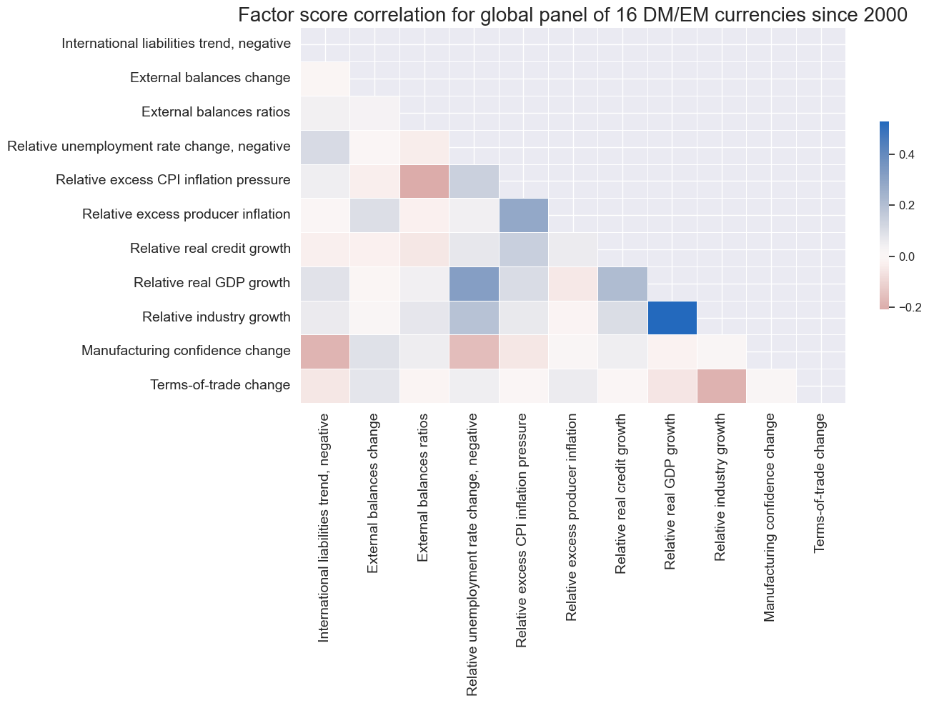
msp.correl_matrix(
dfx_corr,
xcats=list(renaming_dict.values()),
cids=cidx,
start=sdate,
freq="M",
cluster=False,
title="Factor score correlation for global panel of 16 DM/EM currencies since 2000",
size=(14, 10),
)
exts = [
"IIPLIABGDP_D_NEG_ZN",
"XBAL_D_ZN",
"XBALR_ZN",
]
cidx = cids_fx
xcatx = exts
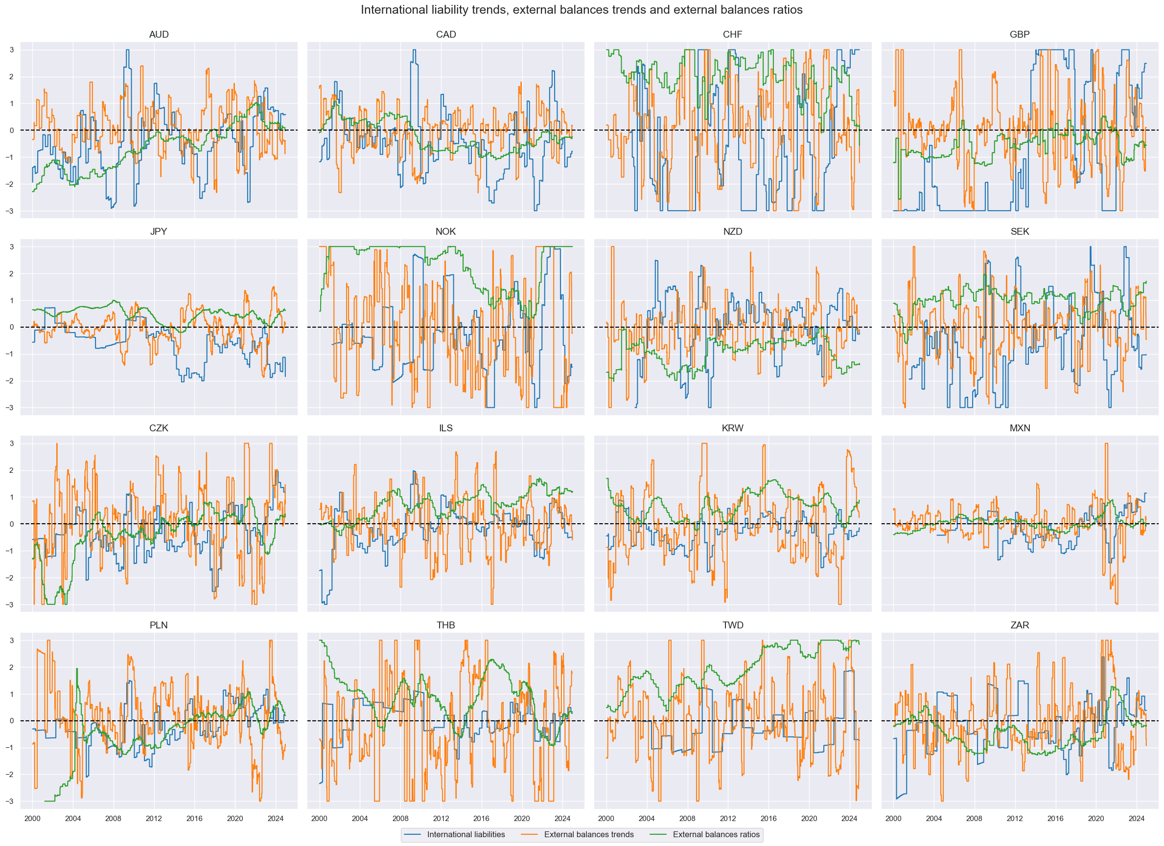
msp.view_timelines(
df=dfx,
xcats=xcatx,
cids=cidx,
start="2000-01-01",
aspect=1.4,
ncol=4,
title = "International liability trends, external balances trends and external balances ratios",
xcat_labels = ["International liabilities", "External balances trends", "External balances ratios"]
)
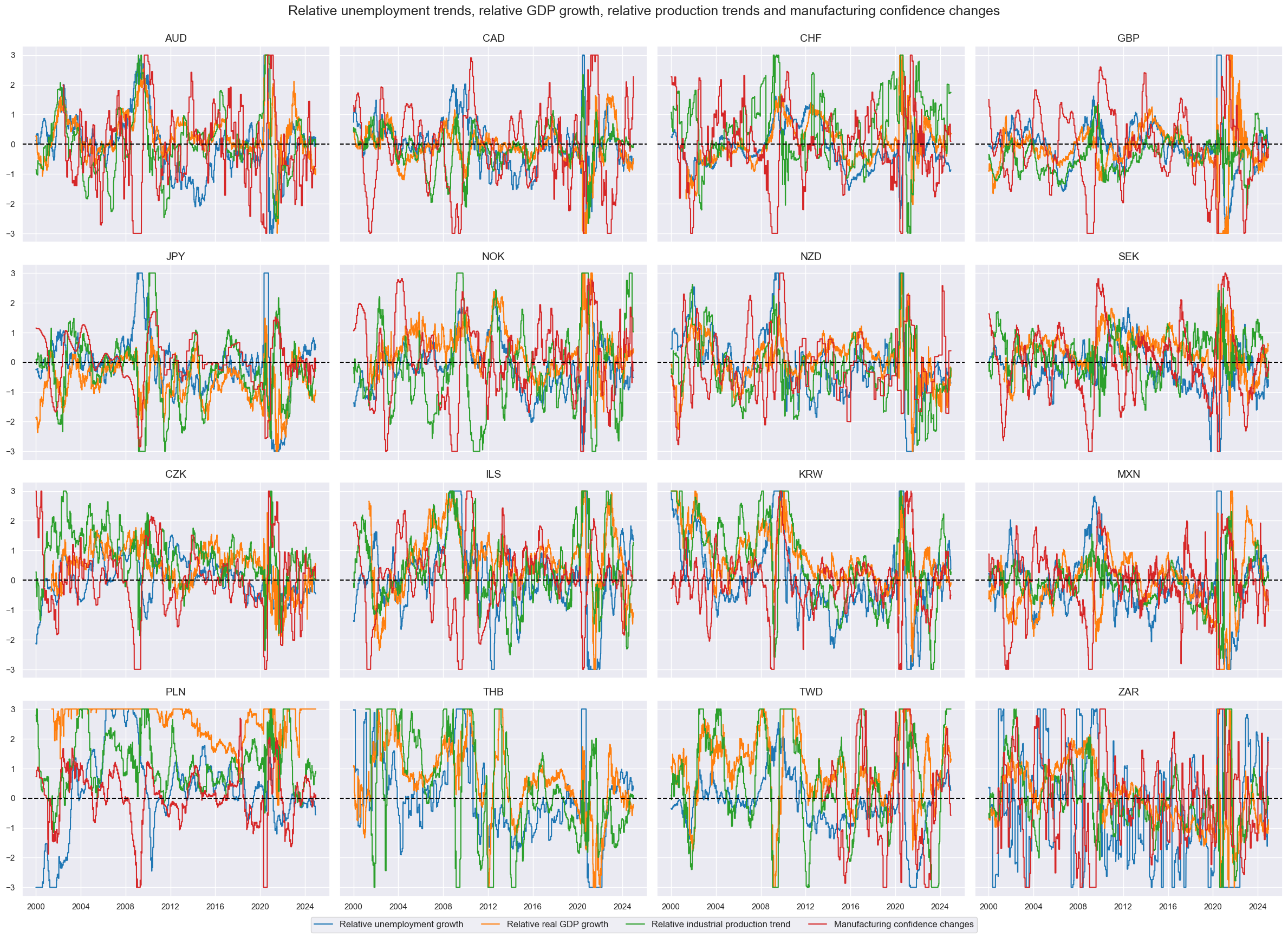
acts = [
    "URATE_DvBM_NEG_ZN",
    "RGDP_PvBM_ZN",
    "IP_PvBM_ZN",
    "MBSCORE_D_ZN",
]

cidx = cids_fx
xcatx = acts

msp.view_timelines(
    df=dfx,
    xcats=xcatx,
    cids=cidx,
    start="2000-01-01",
    aspect=1.4,
    ncol=4,
    title = "Relative unemployment trends, relative GDP growth, relative production trends and manufacturing confidence changes",
    xcat_labels = ["Relative unemployment growth", "Relative real GDP growth", "Relative industrial production trend", "Manufacturing confidence changes"]
)
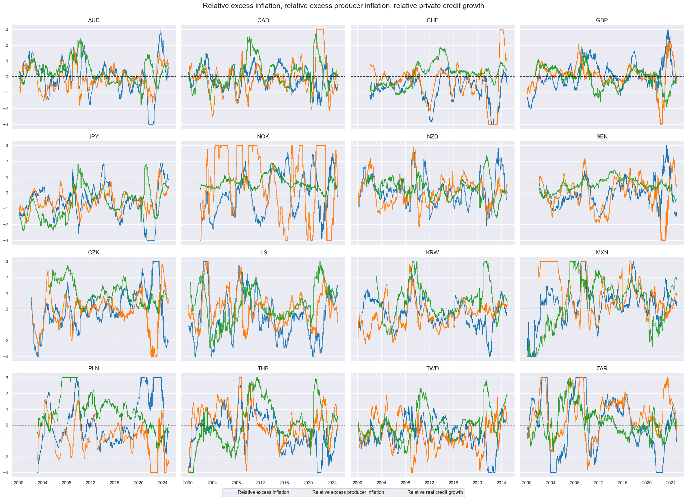
incs = [
    "XINFvBM_ZN",
    "XPPI_PvBM_ZN",
    "RPCREDIT_PvBM_ZN",
]

cidx = cids_fx
xcatx = incs

msp.view_timelines(
    df=dfx,
    xcats=xcatx,
    cids=cidx,
    start="2000-01-01",
    aspect=1.4,
    ncol=4,
    title = "Relative excess inflation, relative excess producer inflation, relative private credit growth",
    xcat_labels = ["Relative excess inflation", "Relative excess producer inflation", "Relative real credit growth"]
)
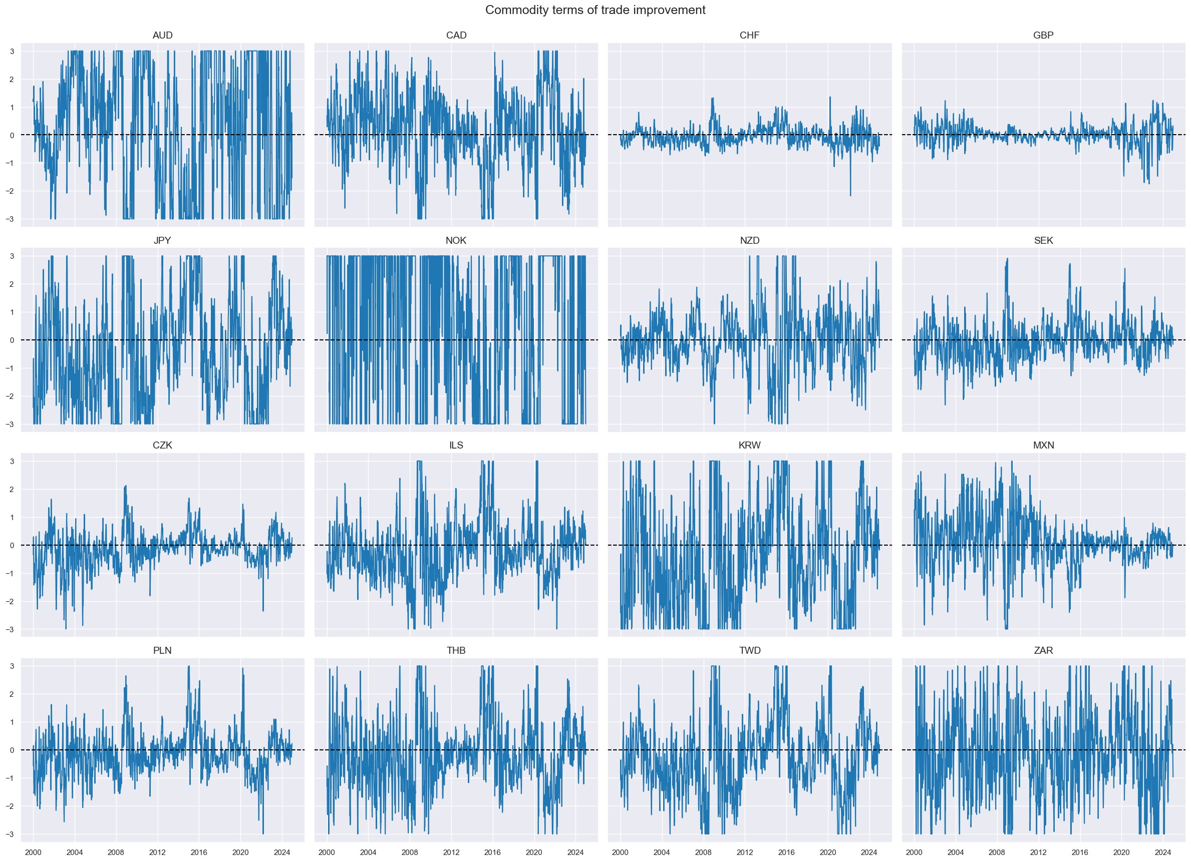
cidx = cids_fx
xcatx = ["CTOT_P_ZN"]

msp.view_timelines(
    df=dfx,
    xcats=xcatx,
    cids=cidx,
    start="2000-01-01",
    aspect=1.4,
    ncol=4,
    title = "Commodity terms of trade improvement",
    xcat_labels = ["Terms of trade improvement"]
)
Availability checks and imputations #
xcatx = [f for f in factorz.keys()]
dfxx = dfx.copy()
msm.check_availability(dfxx, xcatx, missing_recent=False)
cidx = cids_fx
xcatx = ["MBSCORE_D_ZN", "URATE_DvBM_NEG_ZN", "XBALR_ZN"]

dfa = msp.impute_panel(
    dfx, cidx, xcatx, threshold=0.8, impute_empty_tickers=True, start_date="2008-01-01"
)
dfx = msm.update_df(dfx, dfa)
xcatx = [f for f in factorz.keys()]
msm.check_availability(dfx, xcatx, missing_recent=False)
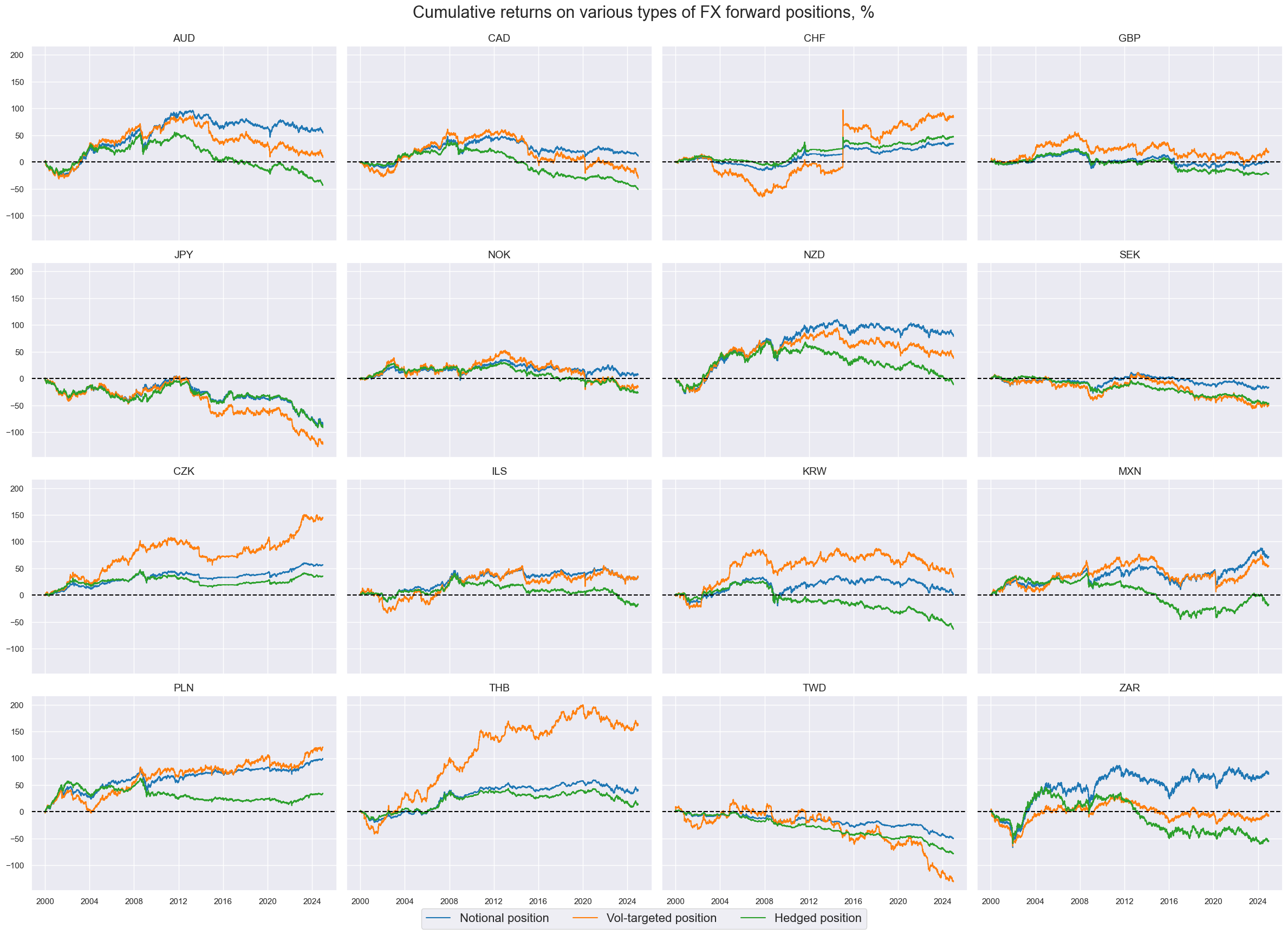
Target return checks #
targs = [
    "FXXR_NSA",
    "FXXR_VT10",
    "FXXRHvGDRB_NSA",
]
xcatx = targs
msm.check_availability(dfx, xcatx, missing_recent=False)
cidx = cids_fx
xcatx = targs

msp.view_timelines(
    df=dfx,
    xcats=xcatx,
    cids=cidx,
    title="Cumulative returns on various types of FX forward positions, %",
    title_fontsize=22,
    xcat_labels=["Notional position", "Vol-targeted position", "Hedged position"],
    cumsum=True,
    start="2000-01-01",
    aspect=1.4,
    ncol=4,
    legend_fontsize = 16,
)
Preparations for statistical learning #
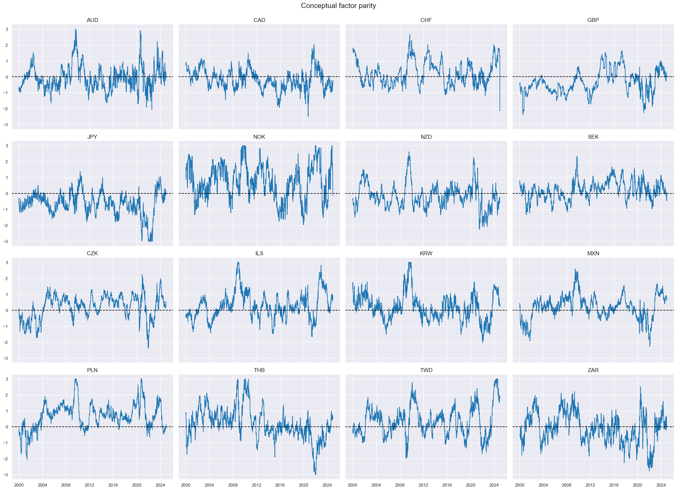
Conceptual parity as benchmark #
# Linear equally-weighted combination of all available candidates

xcatx = [f for f in factorz.keys()]
cidx = cids_fx

dfax = msp.linear_composite(
    df=dfx,
    xcats=xcatx,
    cids=cidx,
    new_xcat="ALL_AVG",
)

dfa = msp.make_zn_scores(
        dfax,
        xcat="ALL_AVG",
        cids=cidx,
        sequential=True,
        min_obs=261 * 3,
        neutral="zero",
        pan_weight=1,
        thresh=3,
        postfix="Z",
        est_freq="m",
    )


dfx = msm.update_df(dfx, dfa)
cidx = cids_fx
xcatx = ["ALL_AVGZ"]

msp.view_timelines(
    df=dfx,
    xcats=xcatx,
    cids=cidx,
    start="2000-01-01",
    aspect=1.4,
    ncol=4,
    title = "Conceptual factor parity",
)
Convert data to scikit-learn format (redundant) #
cidx = cids_fx
targ = "FXXR_VT10"
xcatx = [f for f in factorz.keys()] + [targ]

# Downsample from daily to monthly frequency (features as last and target as sum)
dfw = msm.categories_df(
    df=dfx,
    xcats=xcatx,
    cids=cidx,
    freq="M",
    lag=1,
    blacklist=fxblack,
    xcat_aggs=["last", "sum"],
)

# Drop rows with missing values and assign features and target
dfw.dropna(inplace=True)
X_fx = dfw.iloc[:, :-1]
y_fx = dfw.iloc[:, -1]
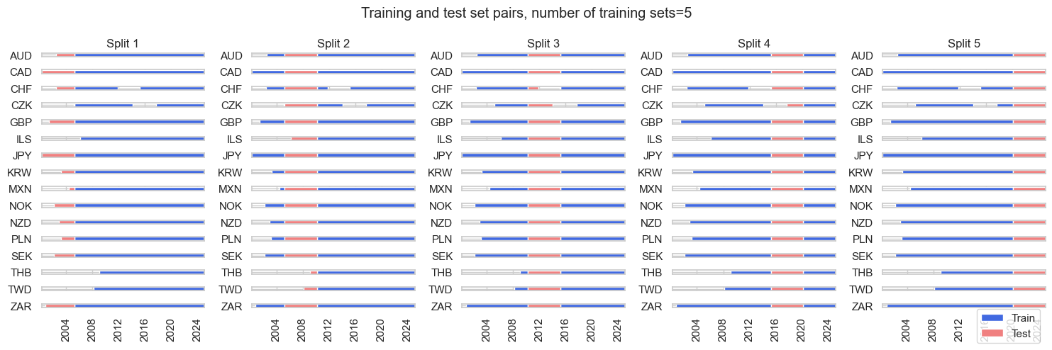
Define splitter and scorer #
splitter = msl.RollingKFoldPanelSplit(n_splits=5)
scorer = make_scorer(msl.sharpe_ratio, greater_is_better=True)
splitter.visualise_splits(X_fx, y_fx, figsize=(15, 5))
Signal generation #
Grids #
# Specify model options and grids

mods_mls = {
    "mls": msl.ModifiedLinearRegression(method="analytic", error_offset=1e-5),
}

grid_mls = {
    "mls": {"positive": [True, False], "fit_intercept": [True, False]},
}
# Random forest grid

mods_rf = {
    "rf_full": RandomForestRegressor(
        n_estimators = 200,
        max_features = "sqrt",
        max_samples = 0.1,
        random_state = 42,
    ),
    "rf_restricted": RandomForestRegressor(
        n_estimators = 200,
        max_features = "sqrt",
        max_samples = 0.1,
        monotonic_cst = [1 for i in range(len(factorz))],
        random_state = 42,
    )
}

grid_rf = {
    "rf_full": {},
    "rf_restricted": {},
}
Learning vol-targeted positions #
# Instantiation

xcatx = [f for f in factorz.keys()] + ["FXXR_VT10"]
cidx = cids_fx

so_fxv = msl.SignalOptimizer(
    df = dfx,
    xcats = xcatx,
    cids = cidx,
    blacklist = fxblack,
    freq = "M",
    lag = 1,
    xcat_aggs = ["last", "sum"]
)
# Learn with linear regression

so_fxv.calculate_predictions(
    name = "LSV",
    models = mods_mls,
    hyperparameters = grid_mls,
    scorers = {"sharpe": scorer},
    inner_splitters = {"Rolling": splitter},
    search_type = "grid",
    normalize_fold_results = False,
    cv_summary = "mean",
    min_cids = 2,
    min_periods = 36,
    test_size = 1,
    n_jobs_outer = -1,
    split_functions={"Rolling": lambda n: n // 36},
)

dfa = so_fxv.get_optimized_signals(name="LSV")
dfx = msm.update_df(dfx, dfa)
# Illustrate model choice
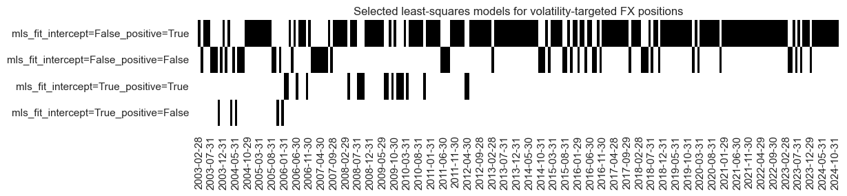
so_fxv.models_heatmap(
"LSV",
title="Selected least-squares models for volatility-targeted FX positions",
figsize=(12, 2),
)
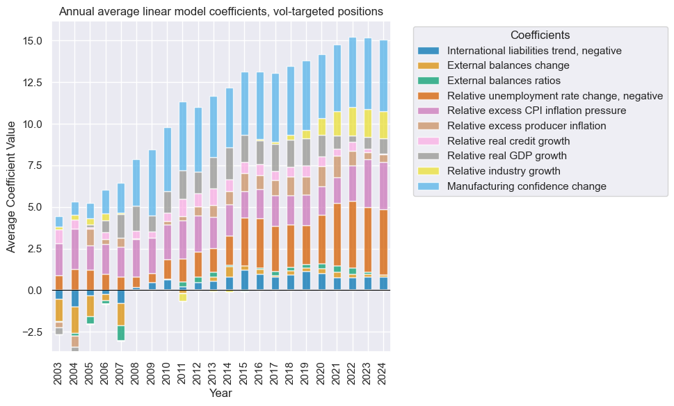
so_fxv.coefs_stackedbarplot(
    "LSV",
    title="Annual average linear model coefficients, vol-targeted positions",
    ftrs_renamed=factorz_labs,
)
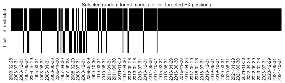
# Learn with random forest

so_fxv.calculate_predictions(
    name = "RFV",
    models = mods_rf,
    hyperparameters = grid_rf,
    scorers = {"sharpe": scorer},
    inner_splitters = {"Rolling": splitter},
    search_type = "grid",
    normalize_fold_results = False,
    cv_summary = "mean",
    min_cids = 2,
    min_periods = 36,
    test_size = 1,
    n_jobs_outer = -1,
)

dfa = so_fxv.get_optimized_signals(name="RFV")
dfx = msm.update_df(dfx, dfa)
# Illustrate model choice

so_fxv.models_heatmap(
    "RFV",
    title="Selected random forest models for vol-targeted FX positions",
    figsize=(12, 2),
)
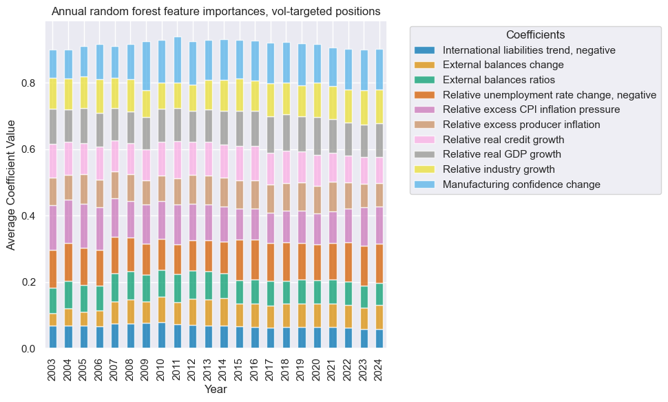
so_fxv.coefs_stackedbarplot(
    "RFV",
    title="Annual random forest feature importances, vol-targeted positions",
    ftrs_renamed=factorz_labs,
)
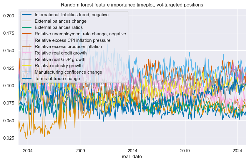
so_fxv.feature_importance_timeplot(
    "RFV",
    title="Random forest feature importance timeplot, vol-targeted positions",
    ftrs_renamed=factorz_labs,
)
# Zn-scores

xcatx = ["LSV", "RFV"]
cidx = cids_fx

dfa = pd.DataFrame(columns=list(dfx.columns))

for xc in xcatx:
    dfaa = msp.make_zn_scores(
        dfx,
        xcat=xc,
        cids=cidx,
        sequential=True,
        min_obs=261 * 3,
        neutral="zero",
        pan_weight=1,
        thresh=3,
        postfix="Z",
        est_freq="m",
    )
    dfa = msm.update_df(dfa, dfaa)

dfx = msm.update_df(dfx, dfa)
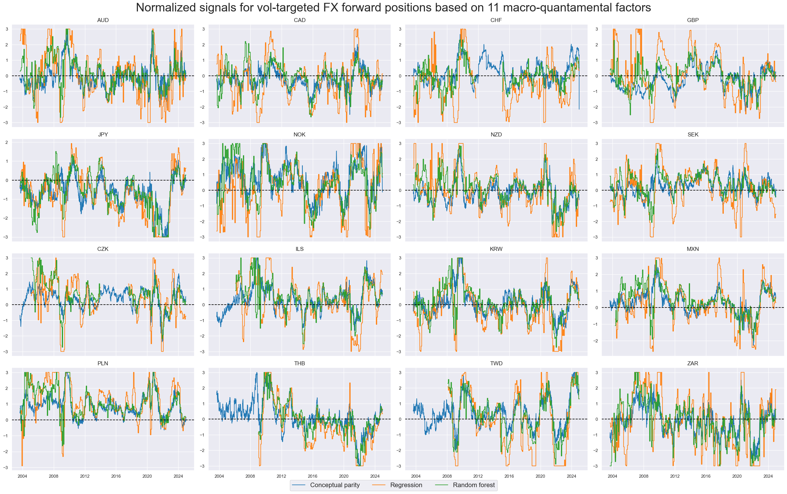
xcatx = ["ALL_AVGZ", "LSVZ", "RFVZ"]
cidx = cids_fx

msp.view_timelines(
    dfx,
    xcats=xcatx,
    cids=cidx,
    ncol=4,
    start="2003-08-29",
    title = "Normalized signals for vol-targeted FX forward positions based on 11 macro-quantamental factors",
    xcat_labels = ["Conceptual parity", "Regression", "Random forest"],
    title_fontsize=30,
    same_y=False,
    cs_mean=False,
    legend_fontsize=16,
)
Learning hedged positions #
# Instantiation

xcatx = [f for f in factorz.keys()]  + ["FXXRHvGDRB_NSA"]
cidx = cids_fx

so_fxh = msl.SignalOptimizer(
    df = dfx,
    xcats = xcatx,
    cids = cidx,
    blacklist = fxblack,
    freq = "M",
    lag = 1,
    xcat_aggs = ["last", "sum"]
)
# Learn with linear regression

so_fxh.calculate_predictions(
    name = "LSH",
    models = mods_mls,
    hyperparameters = grid_mls,
    scorers = {"sharpe": scorer},
    inner_splitters = {"Rolling": splitter},
    search_type = "grid",
    normalize_fold_results = False,
    cv_summary = "mean",
    min_cids = 2,
    min_periods = 36,
    test_size = 1,
    n_jobs_outer = -1,
    split_functions={"Rolling": lambda n: n // 36},
)

dfa = so_fxh.get_optimized_signals(name="LSH")
dfx = msm.update_df(dfx, dfa)
# Illustrate model choice
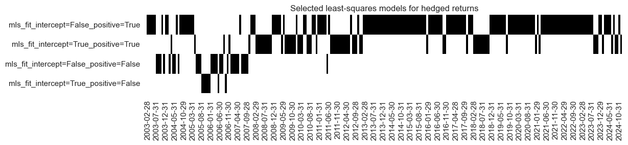
so_fxh.models_heatmap(
"LSH",
title="Selected least-squares models for hedged returns",
figsize=(12, 2),
)
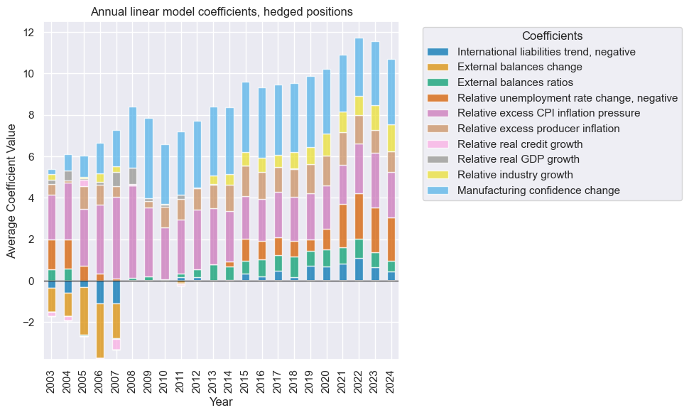
so_fxh.coefs_stackedbarplot(
    "LSH",
    title="Annual linear model coefficients, hedged positions",
    ftrs_renamed=factorz_labs,
)
# Learn with random forest

so_fxh.calculate_predictions(
    name = "RFH",
    models = mods_rf,
    hyperparameters = grid_rf,
    scorers = {"sharpe": scorer},
    inner_splitters = {"Rolling": splitter},
    search_type = "grid",
    normalize_fold_results = False,
    cv_summary = "mean",
    min_cids = 2,
    min_periods = 36,
    test_size = 1,
    n_jobs_outer = -1,
)

dfa = so_fxh.get_optimized_signals()
dfx = msm.update_df(dfx, dfa)
# Illustrate model choice
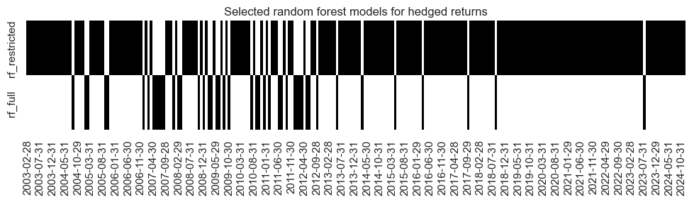
so_fxh.models_heatmap(
"RFH",
title="Selected random forest models for hedged returns",
figsize=(12, 2),
)
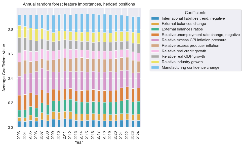
so_fxh.coefs_stackedbarplot(
    "RFH",
    title="Annual random forest feature importances, hedged positions",
    ftrs_renamed=factorz_labs,
)
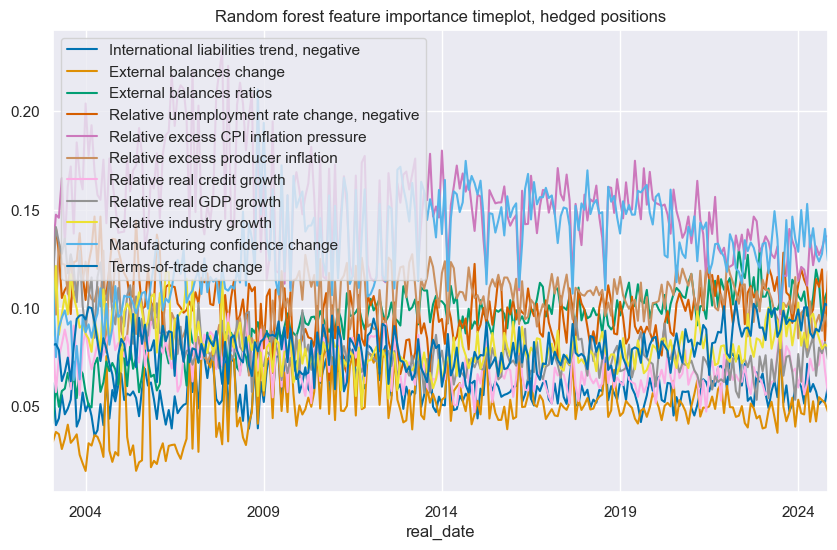
so_fxh.feature_importance_timeplot(
    "RFH",
    title="Random forest feature importance timeplot, hedged positions",
    ftrs_renamed=factorz_labs,
)
# Zn-scores

xcatx = ["LSH", "RFH"]
cidx = cids_fx

dfa = pd.DataFrame(columns=list(dfx.columns))

for xc in xcatx:
    dfaa = msp.make_zn_scores(
        dfx,
        xcat=xc,
        cids=cidx,
        sequential=True,
        min_obs=261 * 3,
        neutral="zero",
        pan_weight=1,
        thresh=3,
        postfix="Z",
        est_freq="m",
    )
    dfa = msm.update_df(dfa, dfaa)

dfx = msm.update_df(dfx, dfa)
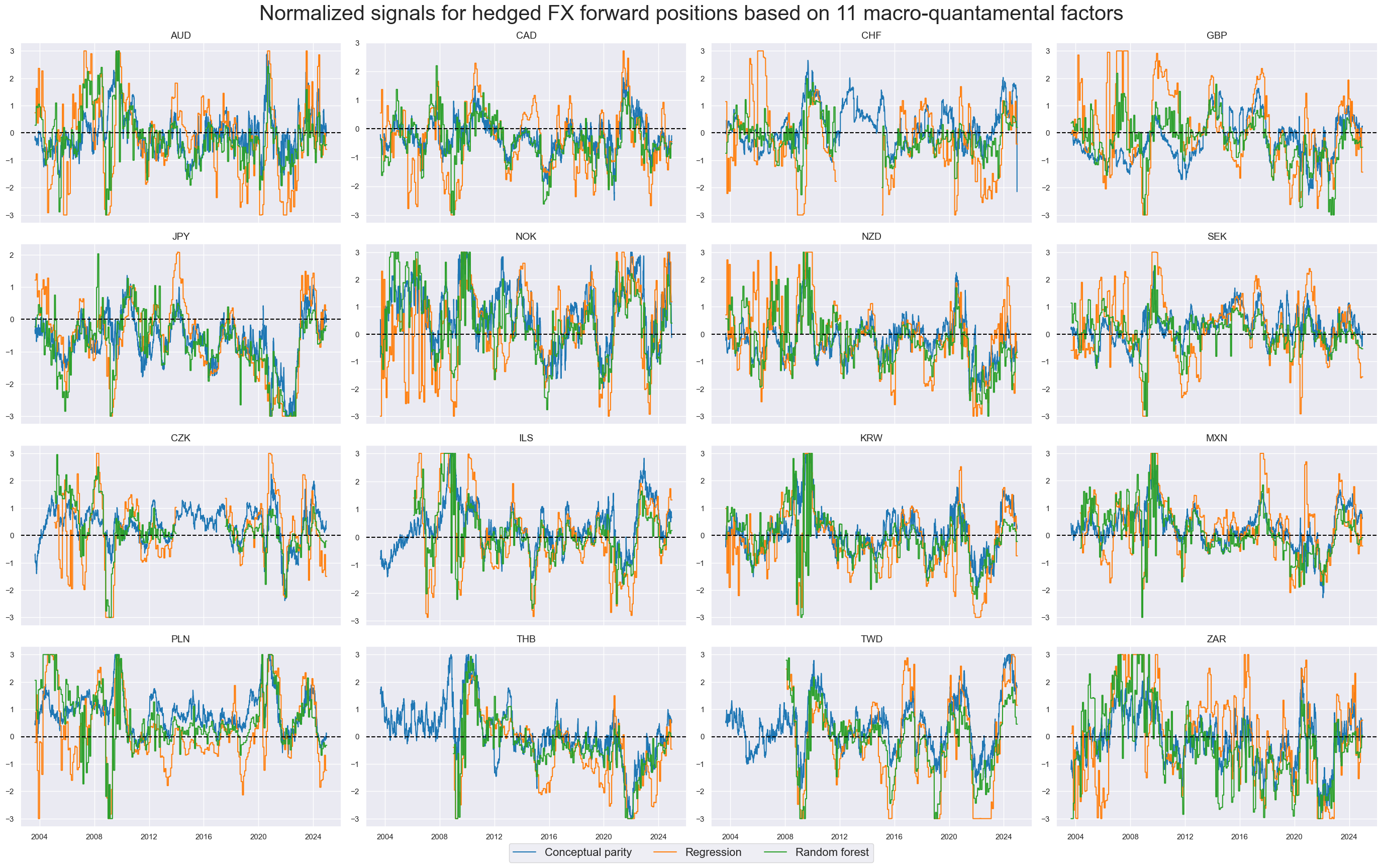
xcatx = ["ALL_AVGZ", "LSHZ", "RFHZ"]
cidx = cids_fx

msp.view_timelines(
    dfx,
    xcats=xcatx,
    cids=cidx,
    ncol=4,
    start="2003-08-29",
    title = "Normalized signals for hedged FX forward positions based on 11 macro-quantamental factors",
    xcat_labels = ["Conceptual parity", "Regression", "Random forest"],
    title_fontsize=30,
    same_y=False,
    cs_mean=False,
    legend_fontsize=16,
)
Signal value checks #
Vol-targeted positions #
Specs and panel test #
cidx = cids_fx
sdate = "2003-08-29"

dict_fxv = {
    "sigs": ["ALL_AVGZ", "LSVZ", "RFVZ"],
    "targs": ["FXXR_VT10"],
    "cidx": cidx,
    "start": sdate,
    "black": fxblack,
    "srr": None,
    "pnls": None,
}
dix = dict_fxv
sigx = dix["sigs"]
tarx = dix["targs"]
cidx = dix["cidx"]
blax = dix["black"]
start = dix["start"]
def crmaker(sig, targ):
crx = msp.CategoryRelations(
dfx,
xcats=[sig, targ],
cids=cidx,
freq="M",
lag=1,
xcat_aggs=["last", "sum"],
start=start,
blacklist=blax,
)
return crx
lcrs = [crmaker(sig, targ) for sig in sigx for targ in tarx]
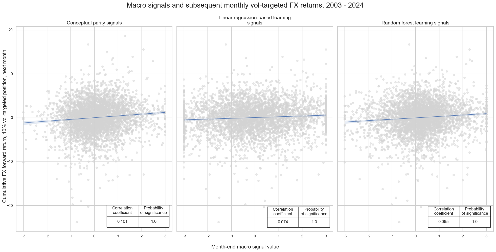
msv.multiple_reg_scatter(
lcrs,
ncol=3,
nrow=1,
figsize=(20, 10),
title="Macro signals and subsequent monthly vol-targeted FX returns, 2003 - 2024",
xlab="Month-end macro signal value",
ylab="Cumulative FX forward return, 10% vol-targeted position, next month",
coef_box="lower right",
prob_est="map",
subplot_titles=[
"Conceptual parity signals",
"Linear regression-based learning signals",
"Random forest learning signals",
],
)
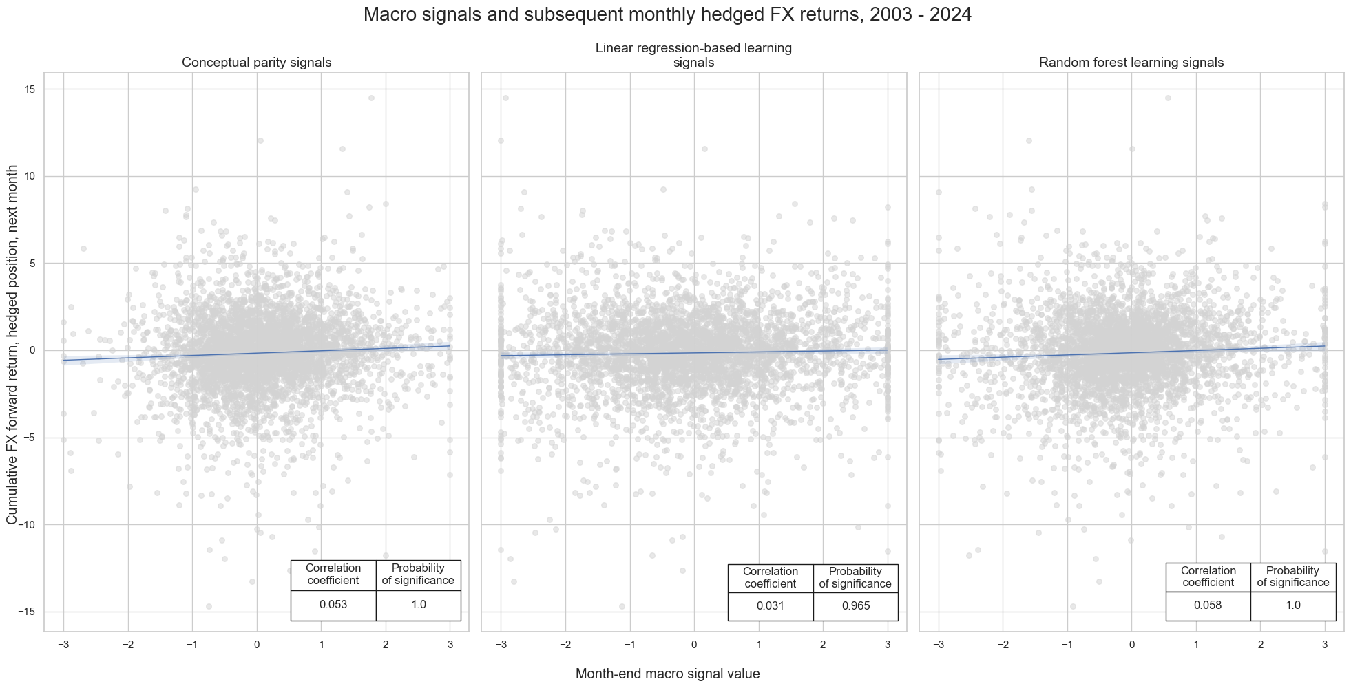
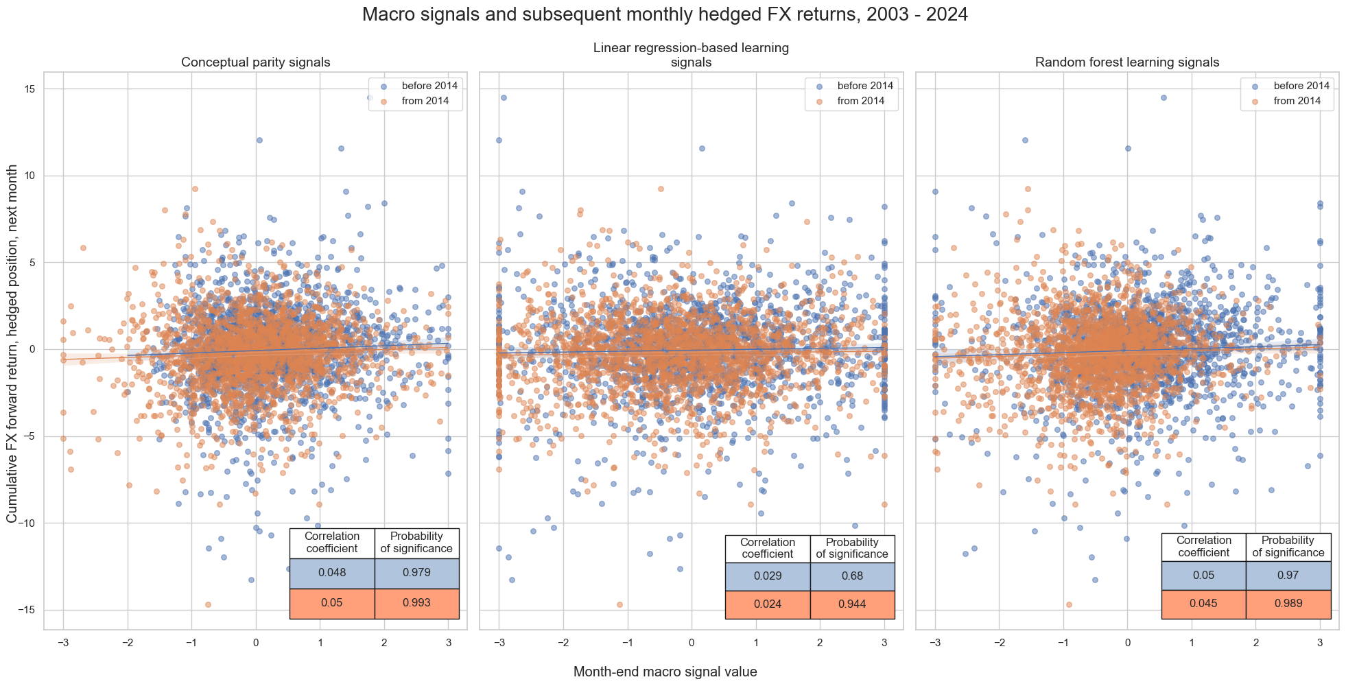
msv.multiple_reg_scatter(
lcrs,
ncol=3,
nrow=1,
figsize=(20, 10),
title="Macro signals and subsequent monthly hedged FX returns, 2003 - 2024",
xlab="Month-end macro signal value",
ylab="Cumulative FX forward return, 10% vol-targeted position, next month",
coef_box="lower right",
prob_est="map",
subplot_titles=[
"Conceptual parity signals",
"Linear regression-based learning signals",
"Random forest learning signals",
],
separator=2014,
)
dix = dict_fxv
sigx = dix["sigs"]
tarx = dix["targs"]
cidx = dix["cidx"]
blax = dix["black"]
start = dix["start"]
def crmaker(sig, targ):
crx = msp.CategoryRelations(
dfx,
xcats=[sig, targ],
cids=cidx,
freq="Q",
lag=1,
xcat_aggs=["last", "sum"],
start=start,
blacklist=blax,
)
return crx
lcrs = [crmaker(sig, targ) for sig in sigx for targ in tarx]
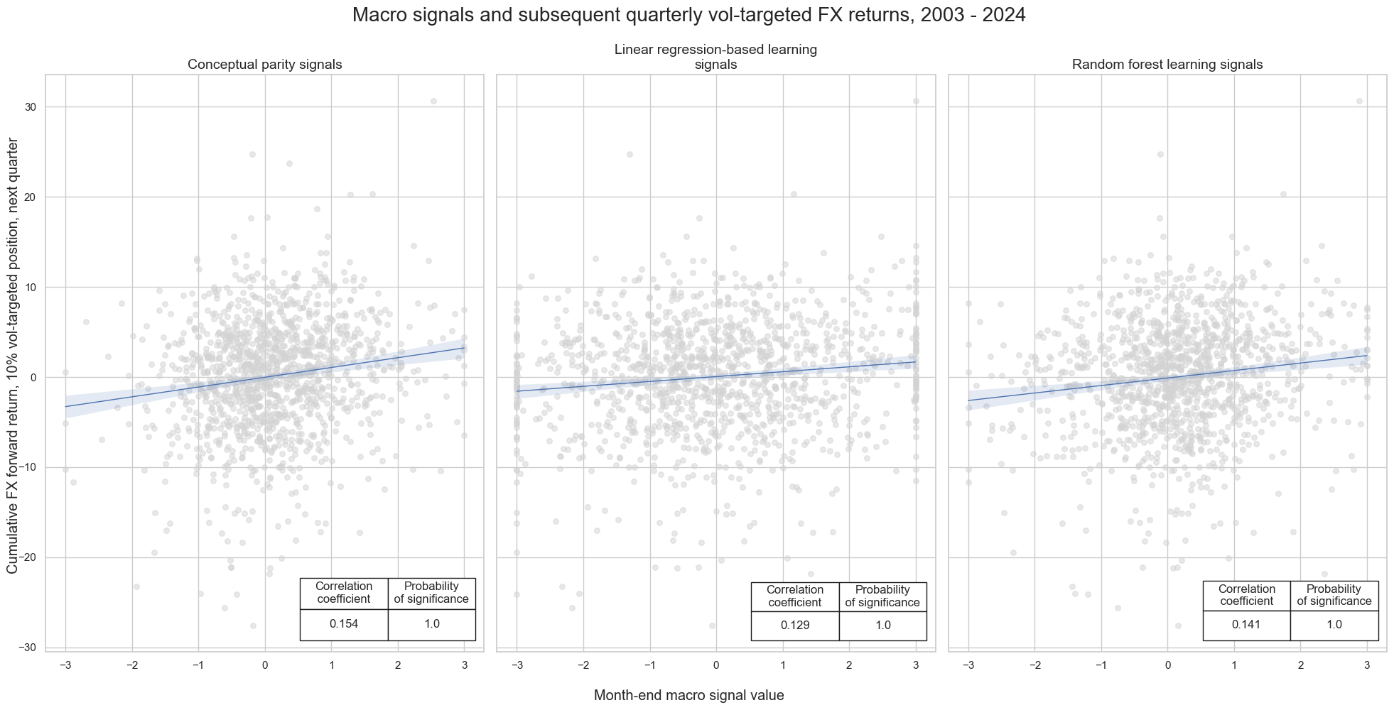
msv.multiple_reg_scatter(
lcrs,
ncol=3,
nrow=1,
figsize=(20, 10),
title="Macro signals and subsequent quarterly vol-targeted FX returns, 2003 - 2024",
xlab="Month-end macro signal value",
ylab="Cumulative FX forward return, 10% vol-targeted position, next quarter",
coef_box="lower right",
prob_est="map",
subplot_titles=[
"Conceptual parity signals",
"Linear regression-based learning signals",
"Random forest learning signals",
],
)
msv.multiple_reg_scatter(
lcrs,
ncol=3,
nrow=1,
figsize=(20, 10),
title="Macro signals and subsequent quarterly vol-targeted FX returns, 2003 - 2024",
xlab="Month-end macro signal value",
ylab="Cumulative FX forward return, 10% vol-targeted position, next quarter",
coef_box="lower right",
prob_est="map",
subplot_titles=[
"Conceptual parity signals",
"Linear regression-based learning signals",
"Random forest learning signals",
],
separator=2014,
)
Accuracy and correlation check #
## Compare optimized signals with simple average z-scores

dix = dict_fxv

sigx = dix["sigs"]
tarx = dix["targs"]
cidx = dix["cidx"]
blax = dix["black"]
startx = dix["start"]

srr = mss.SignalReturnRelations(
    df=dfx,
    rets=tarx,
    sigs=sigx,
    cids=cidx,
    cosp=True,
    freqs=["M"],
    agg_sigs=["last"],
    start=startx,
    blacklist=blax,
    slip=1,
    ms_panel_test=True,
)
dix["srr"] = srr

selcols = [
    "accuracy",
    "bal_accuracy",
    "pos_sigr",
    "pos_retr",
    "pearson",
    "map_pval",
    "kendall",
    "kendall_pval",
]

srr.multiple_relations_table().round(3)[selcols]
| accuracy | bal_accuracy | pos_sigr | pos_retr | pearson | map_pval | kendall | kendall_pval | ||||
|---|---|---|---|---|---|---|---|---|---|---|---|
| Return | Signal | Frequency | Aggregation | ||||||||
| FXXR_VT10 | ALL_AVGZ | M | last | 0.531 | 0.530 | 0.528 | 0.522 | 0.095 | 0.0 | 0.059 | 0.0 |
| LSVZ | M | last | 0.512 | 0.513 | 0.487 | 0.522 | 0.071 | 0.0 | 0.041 | 0.0 | |
| RFVZ | M | last | 0.526 | 0.523 | 0.601 | 0.522 | 0.098 | 0.0 | 0.060 | 0.0 |
Naive PnL #
dix = dict_fxv

sigx = dix["sigs"]
tarx = dix["targs"]
cidx = dix["cidx"]
blax = dix["black"]
startx = dix["start"]

pnls = msn.NaivePnL(
    df=dfx,
    ret=tarx[0],
    sigs=sigx,
    cids=cidx,
    start=startx,
    blacklist=blax,
    bms=["USD_GB10YXR_NSA", "EUR_FXXR_NSA", "USD_EQXR_NSA"],
)
for sig in sigx:
    pnls.make_pnl(
        sig=sig,
        sig_op="raw",
        rebal_freq="monthly",
        neutral="zero",
        rebal_slip=1,
        vol_scale=10,
    )
pnls.make_long_pnl(vol_scale=10, label="Long only")

dix['pnls'] = pnls
dix = dict_fxv
pnls = dict_fxv["pnls"]
sigx = dix["sigs"]

pnls.plot_pnls(
    title="Naive PnLs of vol-targeted FX forward positions based on macro signals",
    title_fontsize=14,
    xcat_labels=[
        "Conceptual parity",
        "Linear regression-based learning",
        "Random forest-based learning",
        "Long only",
    ],
)
pnls.evaluate_pnls(pnl_cats=["PNL_" + sig for sig in sigx] + ["Long only"])
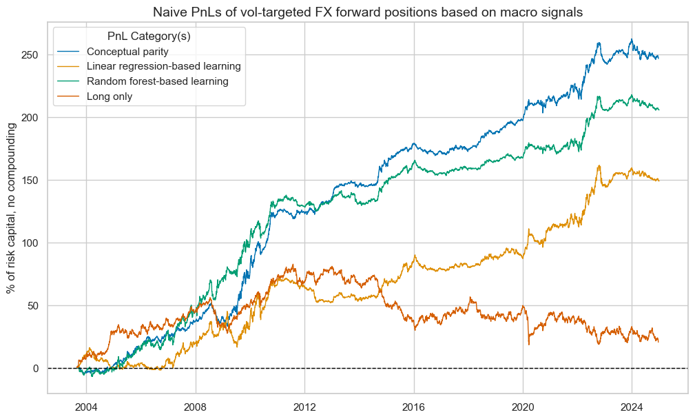
| xcat | PNL_ALL_AVGZ | PNL_LSVZ | PNL_RFVZ | Long only |
|---|---|---|---|---|
| Return % | 11.573196 | 6.991206 | 9.645992 | 0.967029 |
| St. Dev. % | 10.0 | 10.0 | 10.0 | 10.0 |
| Sharpe Ratio | 1.15732 | 0.699121 | 0.964599 | 0.096703 |
| Sortino Ratio | 1.759249 | 1.013046 | 1.414893 | 0.132339 |
| Max 21-Day Draw % | -11.562754 | -20.972745 | -14.553378 | -24.329186 |
| Max 6-Month Draw % | -14.960068 | -18.956451 | -10.168273 | -24.479089 |
| Peak to Trough Draw % | -18.687284 | -28.622746 | -15.973817 | -64.270266 |
| Top 5% Monthly PnL Share | 0.479377 | 0.724625 | 0.519515 | 4.494745 |
| USD_GB10YXR_NSA correl | -0.107952 | -0.05807 | -0.063287 | -0.008622 |
| EUR_FXXR_NSA correl | -0.014618 | -0.042602 | 0.030355 | 0.505311 |
| USD_EQXR_NSA correl | 0.135619 | 0.000256 | 0.064407 | 0.283902 |
| Traded Months | 257 | 257 | 257 | 257 |
dix = dict_fxv
pnls = dix["pnls"]
sigx = dix["sigs"]


pnls.plot_pnls(pnl_cats=["PNL_RFVZ"], pnl_cids=cids_fx, facet=True, title = "Vol-targeted FX PnLs for each currency area, random forest signal")
pnls.evaluate_pnls(pnl_cats=["PNL_RFVZ"], pnl_cids=cids_fx)
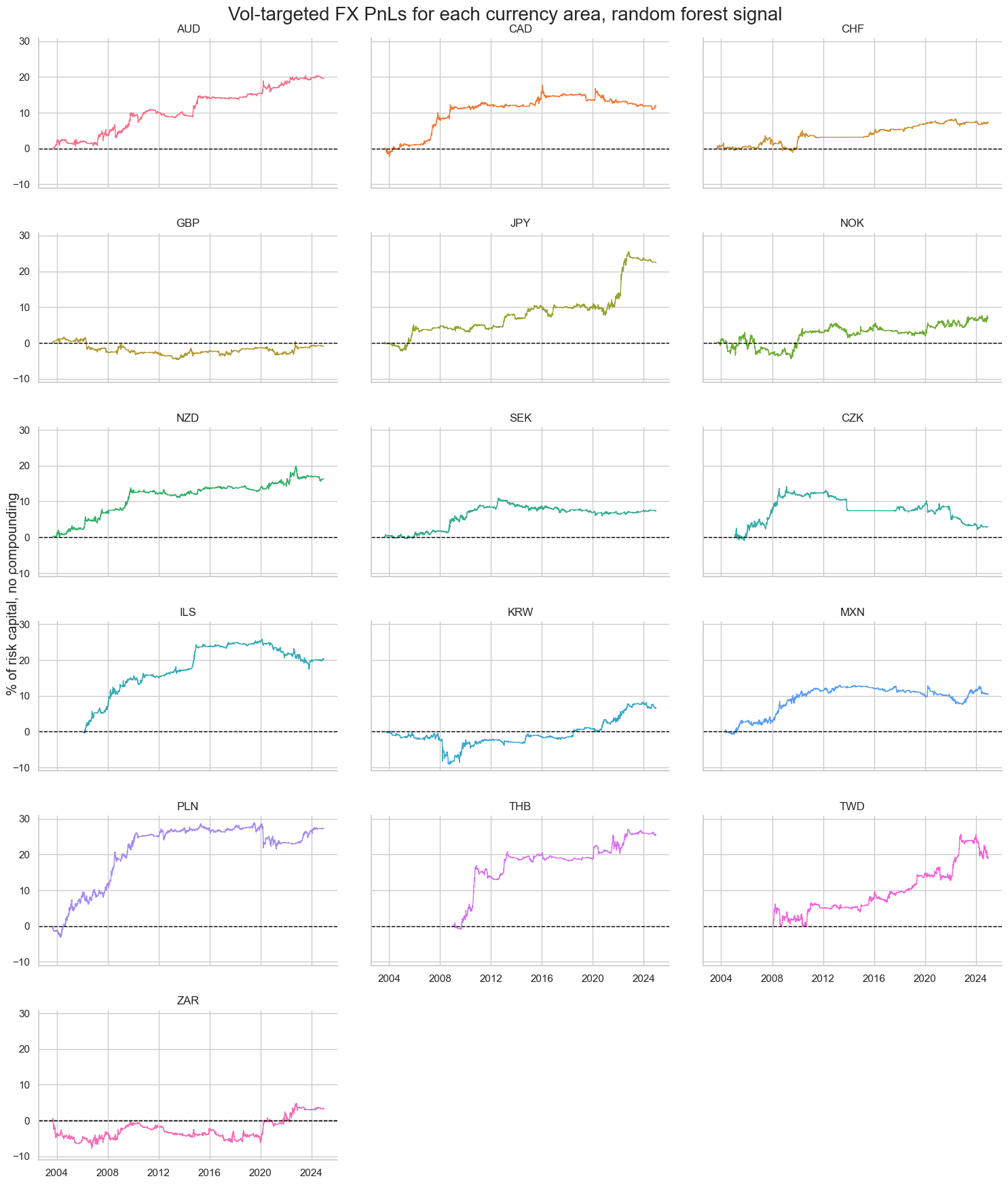
| cid | AUD | CAD | CHF | CZK | GBP | ILS | JPY | KRW | MXN | NOK | NZD | PLN | SEK | THB | TWD | ZAR |
|---|---|---|---|---|---|---|---|---|---|---|---|---|---|---|---|---|
| Return % | 0.916191 | 0.563574 | 0.40357 | 0.181651 | -0.041862 | 1.069398 | 1.050794 | 0.304151 | 0.51101 | 0.32508 | 0.766878 | 1.283235 | 0.345011 | 1.588763 | 1.116021 | 0.149844 |
| St. Dev. % | 1.606308 | 1.419869 | 1.316372 | 1.99747 | 1.276242 | 1.80057 | 1.960339 | 1.714892 | 1.56284 | 2.222054 | 1.497604 | 2.33447 | 1.323055 | 1.975754 | 2.417985 | 2.062155 |
| Sharpe Ratio | 0.570371 | 0.39692 | 0.306578 | 0.090941 | -0.032801 | 0.593922 | 0.536027 | 0.177359 | 0.326975 | 0.146297 | 0.51207 | 0.54969 | 0.260769 | 0.80413 | 0.46155 | 0.072664 |
| Sortino Ratio | 0.823092 | 0.575731 | 0.472787 | 0.143537 | -0.04618 | 0.937302 | 0.796399 | 0.242347 | 0.462236 | 0.206906 | 0.741676 | 0.790419 | 0.378639 | 1.466272 | 0.769407 | 0.104174 |
| Max 21-Day Draw % | -3.502589 | -2.172801 | -2.21007 | -3.077397 | -2.586212 | -2.049386 | -1.982875 | -5.79044 | -2.036673 | -3.027575 | -2.601862 | -5.961496 | -1.18196 | -3.585332 | -4.533752 | -3.041174 |
| Max 6-Month Draw % | -2.470959 | -3.162021 | -2.164 | -3.605455 | -3.302787 | -2.819012 | -2.510821 | -7.106388 | -2.55023 | -4.89763 | -3.452304 | -4.858807 | -1.262605 | -4.212953 | -6.066868 | -4.811437 |
| Peak to Trough Draw % | -3.804048 | -6.812088 | -4.795057 | -11.963634 | -6.325556 | -8.464626 | -3.280933 | -9.272184 | -5.382261 | -7.451822 | -4.249911 | -7.43646 | -5.05745 | -5.249365 | -6.915655 | -8.481324 |
| Top 5% Monthly PnL Share | 0.837075 | 1.449536 | 1.606123 | 6.425507 | -11.725726 | 1.007353 | 1.06243 | 2.412736 | 1.193445 | 2.712075 | 1.080883 | 0.879976 | 1.736402 | 1.192052 | 1.58733 | 6.780772 |
| USD_GB10YXR_NSA correl | -0.011597 | -0.031706 | -0.005453 | 0.009301 | 0.017541 | 0.040662 | -0.159795 | -0.030107 | -0.074606 | -0.005592 | -0.05054 | -0.052828 | -0.015632 | -0.004054 | 0.0161 | 0.008854 |
| EUR_FXXR_NSA correl | 0.057203 | -0.100224 | 0.040467 | 0.045255 | -0.11448 | 0.238139 | -0.213114 | 0.026429 | 0.092679 | 0.016609 | 0.090237 | 0.114813 | -0.050312 | -0.01881 | 0.041415 | -0.088263 |
| USD_EQXR_NSA correl | -0.003128 | -0.069028 | 0.018508 | 0.037521 | -0.054222 | 0.092203 | 0.06142 | 0.028468 | 0.103331 | 0.006571 | 0.028785 | 0.154093 | 0.045762 | -0.015967 | -0.023483 | -0.075457 |
| Traded Months | 257 | 257 | 257 | 257 | 257 | 257 | 257 | 257 | 257 | 257 | 257 | 257 | 257 | 257 | 257 | 257 |
Hedged positions #
Specs and panel test #
cidx = cids_fx
sdate = "2003-08-29"

dict_fxh = {
    "sigs": ["ALL_AVGZ", "LSHZ", "RFHZ"],
    "targs": ["FXXRHvGDRB_NSA"],
    "cidx": cidx,
    "start": sdate,
    "black": fxblack,
    "srr": None,
    "pnls": None,
}
dix = dict_fxh
sigx = dix["sigs"]
tarx = dix["targs"]
cidx = dix["cidx"]
blax = dix["black"]
start = dix["start"]
def crmaker(sig, targ):
crx = msp.CategoryRelations(
dfx,
xcats=[sig, targ],
cids=cidx,
freq="M",
lag=1,
xcat_aggs=["last", "sum"],
start=start,
blacklist=blax,
)
return crx
lcrs = [crmaker(sig, targ) for sig in sigx for targ in tarx]
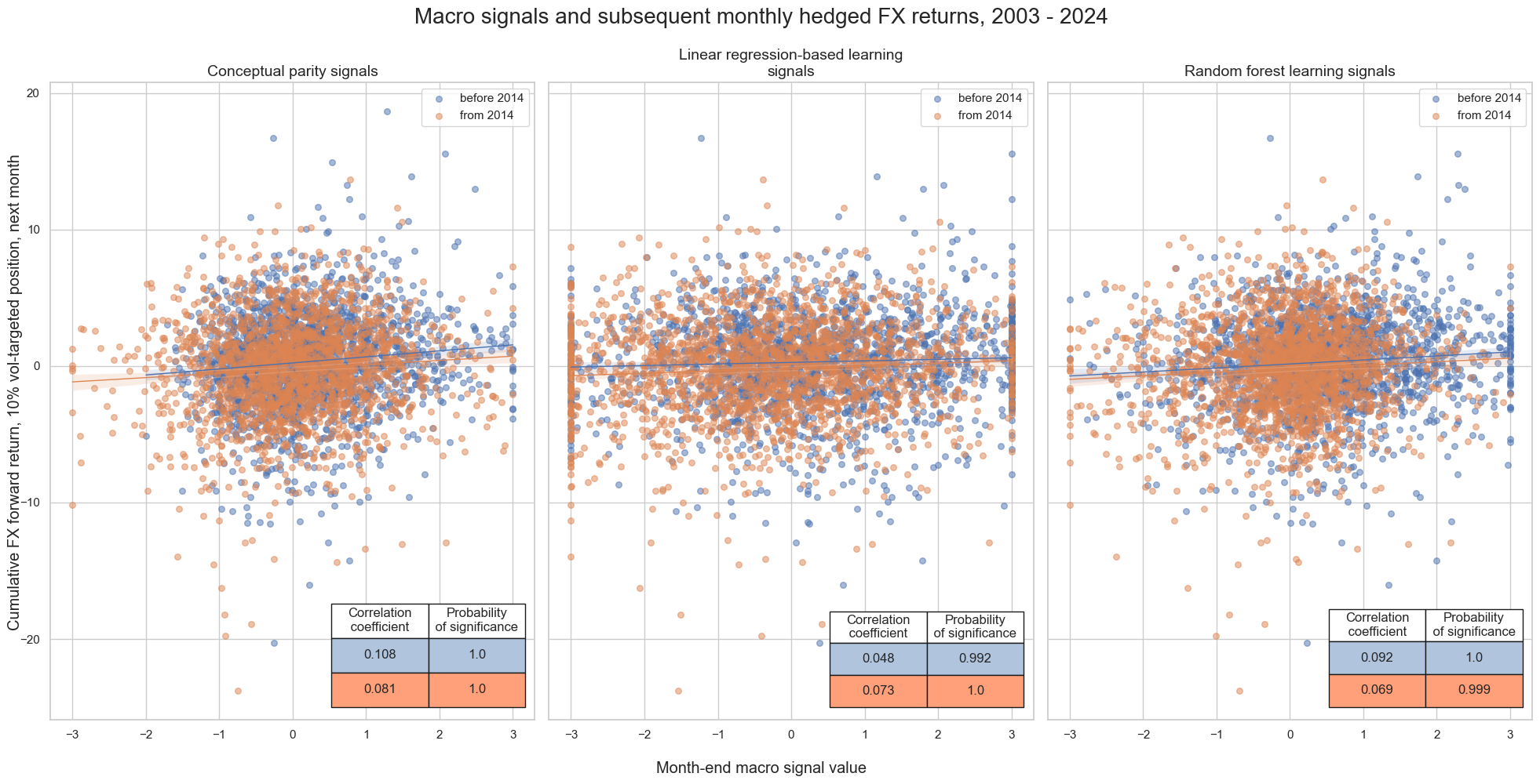
msv.multiple_reg_scatter(
lcrs,
ncol=3,
nrow=1,
figsize=(20, 10),
title="Macro signals and subsequent monthly hedged FX returns, 2003 - 2024",
xlab="Month-end macro signal value",
ylab="Cumulative FX forward return, hedged position, next month",
coef_box="lower right",
prob_est="map",
subplot_titles=[
"Conceptual parity signals",
"Linear regression-based learning signals",
"Random forest learning signals",
],
)
msv.multiple_reg_scatter(
lcrs,
ncol=3,
nrow=1,
figsize=(20, 10),
title="Macro signals and subsequent monthly hedged FX returns, 2003 - 2024",
xlab="Month-end macro signal value",
ylab="Cumulative FX forward return, hedged position, next month",
coef_box="lower right",
prob_est="map",
subplot_titles=[
"Conceptual parity signals",
"Linear regression-based learning signals",
"Random forest learning signals",
],
separator=2014,
)
dix = dict_fxh
sigx = dix["sigs"]
tarx = dix["targs"]
cidx = dix["cidx"]
blax = dix["black"]
start = dix["start"]
def crmaker(sig, targ):
crx = msp.CategoryRelations(
dfx,
xcats=[sig, targ],
cids=cidx,
freq="Q",
lag=1,
xcat_aggs=["last", "sum"],
start=start,
blacklist=blax,
)
return crx
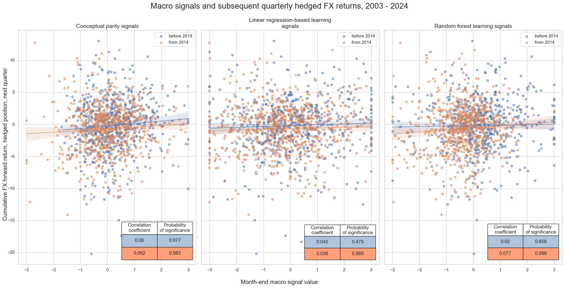
lcrs = [crmaker(sig, targ) for sig in sigx for targ in tarx]
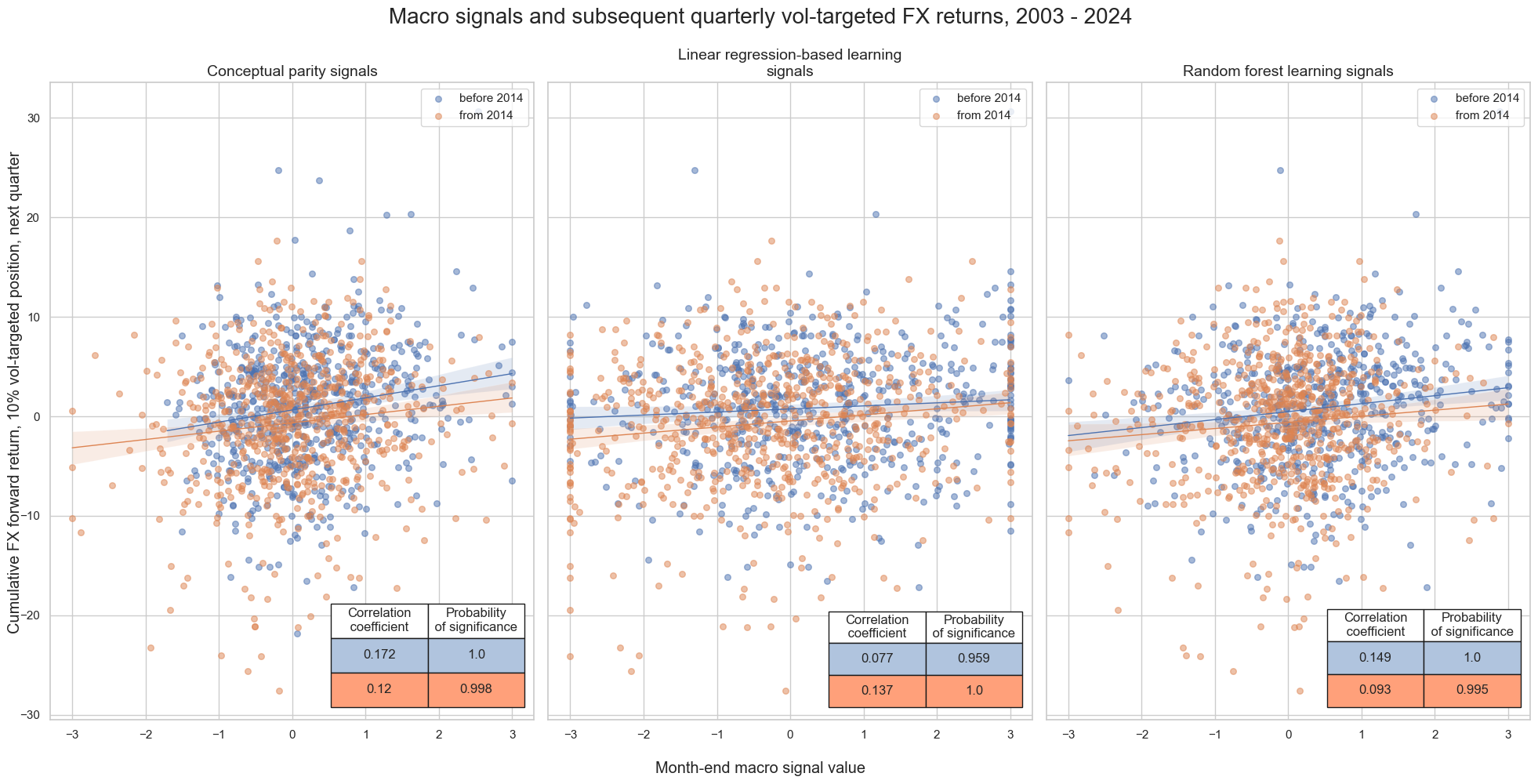
msv.multiple_reg_scatter(
lcrs,
ncol=3,
nrow=1,
figsize=(20, 10),
title="Macro signals and subsequent quarterly hedged FX returns, 2003 - 2024",
xlab="Month-end macro signal value",
ylab="Cumulative FX forward return, hedged position, next quarter",
coef_box="lower right",
prob_est="map",
subplot_titles=[
"Conceptual parity signals",
"Linear regression-based learning signals",
"Random forest learning signals",
],
)
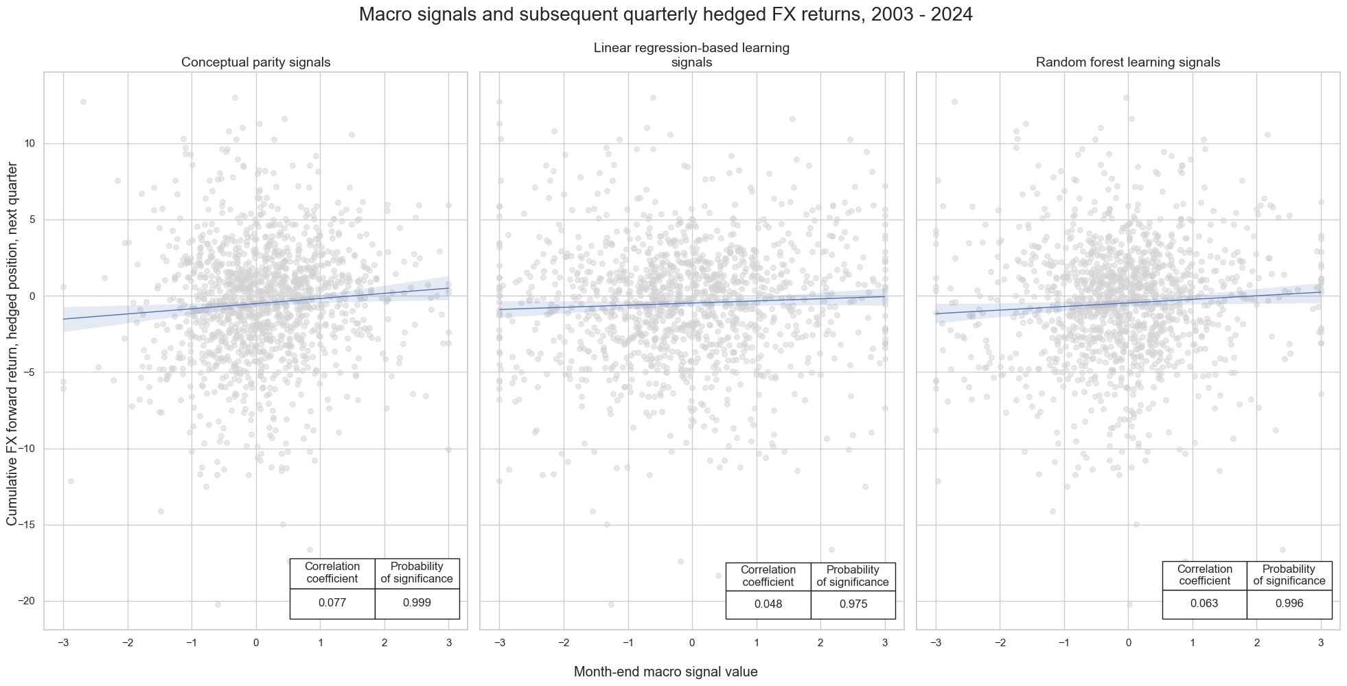
msv.multiple_reg_scatter(
lcrs,
ncol=3,
nrow=1,
figsize=(20, 10),
title="Macro signals and subsequent quarterly hedged FX returns, 2003 - 2024",
xlab="Month-end macro signal value",
ylab="Cumulative FX forward return, hedged position, next quarter",
coef_box="lower right",
prob_est="map",
subplot_titles=[
"Conceptual parity signals",
"Linear regression-based learning signals",
"Random forest learning signals",
],
separator=2014,
)
Accuracy and correlation check #
## Compare optimized signals with simple average z-scores

dix = dict_fxh

sigx = dix["sigs"]
tarx = dix["targs"]
cidx = dix["cidx"]
blax = dix["black"]
startx = dix["start"]

srr = mss.SignalReturnRelations(
    df=dfx,
    rets=tarx,
    sigs=sigx,
    cids=cidx,
    cosp=True,
    freqs=["M"],
    agg_sigs=["last"],
    start=startx,
    blacklist=blax,
    slip=1,
    ms_panel_test=True,
)
dix["srr"] = srr

selcols = [
    "accuracy",
    "bal_accuracy",
    "pos_sigr",
    "pos_retr",
    "pearson",
    "map_pval",
    "kendall",
    "kendall_pval",
]

srr.multiple_relations_table().round(3)[selcols]
| accuracy | bal_accuracy | pos_sigr | pos_retr | pearson | map_pval | kendall | kendall_pval | ||||
|---|---|---|---|---|---|---|---|---|---|---|---|
| Return | Signal | Frequency | Aggregation | ||||||||
| FXXRHvGDRB_NSA | ALL_AVGZ | M | last | 0.528 | 0.529 | 0.528 | 0.482 | 0.049 | 0.000 | 0.042 | 0.000 |
| LSHZ | M | last | 0.509 | 0.508 | 0.467 | 0.482 | 0.028 | 0.038 | 0.018 | 0.091 | |
| RFHZ | M | last | 0.534 | 0.532 | 0.453 | 0.482 | 0.053 | 0.001 | 0.047 | 0.000 |
Naive PnL #
dix = dict_fxh

sigx = dix["sigs"]
tarx = dix["targs"]
cidx = dix["cidx"]
blax = dix["black"]
startx = dix["start"]

pnls = msn.NaivePnL(
    df=dfx,
    ret=tarx[0],
    sigs=sigx,
    cids=cidx,
    start=startx,
    blacklist=blax,
    bms=["USD_GB10YXR_NSA", "EUR_FXXR_NSA", "USD_EQXR_NSA"],
)
for sig in sigx:
    pnls.make_pnl(
        sig=sig,
        sig_op="raw",
        rebal_freq="monthly",
        neutral="zero",
        rebal_slip=1,
        vol_scale=10,
    )
pnls.make_long_pnl(vol_scale=10, label="Long only")

dix["pnls"] = pnls
dix = dict_fxh
pnls = dix["pnls"]
sigx = dix["sigs"]

pnls.plot_pnls(
    title="Naive PnLs of hedged FX forward positions based on macro signals",
    title_fontsize=14,
    xcat_labels=[
        "Conceptual parity",
        "Linear regression-based learning",
        "Random forest-based learning",
        "Long only",
    ],
)
pnls.evaluate_pnls(pnl_cats=["PNL_" + sig for sig in sigx] + ["Long only"])
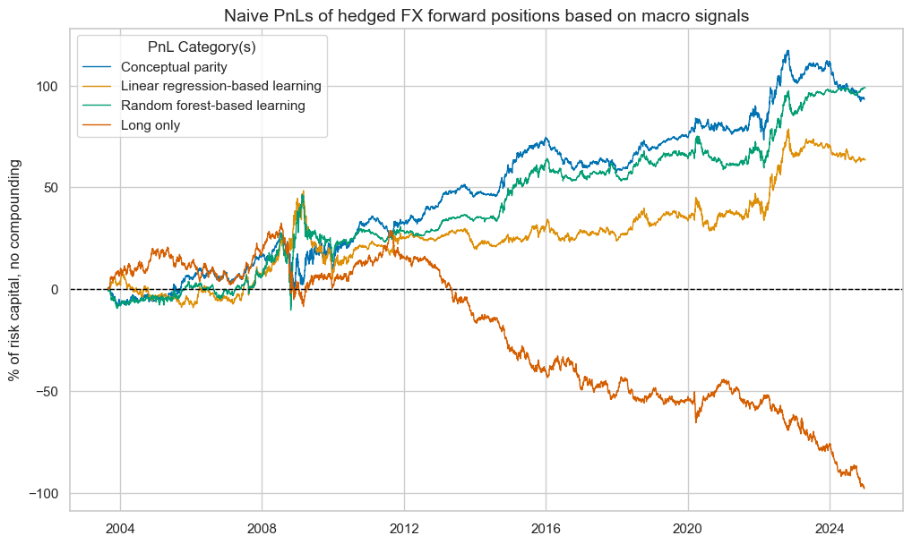
| xcat | PNL_ALL_AVGZ | PNL_LSHZ | PNL_RFHZ | Long only |
|---|---|---|---|---|
| Return % | 4.371751 | 2.97701 | 4.635429 | -4.595695 |
| St. Dev. % | 10.0 | 10.0 | 10.0 | 10.0 |
| Sharpe Ratio | 0.437175 | 0.297701 | 0.463543 | -0.45957 |
| Sortino Ratio | 0.634468 | 0.419443 | 0.647475 | -0.628564 |
| Max 21-Day Draw % | -20.193632 | -15.243791 | -26.888151 | -23.712188 |
| Max 6-Month Draw % | -23.852403 | -28.851387 | -24.264262 | -33.29414 |
| Peak to Trough Draw % | -28.924819 | -43.47515 | -38.002827 | -130.39716 |
| Top 5% Monthly PnL Share | 1.080057 | 1.597565 | 1.059348 | -0.660979 |
| USD_GB10YXR_NSA correl | -0.07334 | -0.0184 | -0.061603 | 0.149457 |
| EUR_FXXR_NSA correl | -0.079704 | -0.18641 | -0.166692 | 0.499291 |
| USD_EQXR_NSA correl | 0.036703 | -0.039598 | 0.008995 | -0.089722 |
| Traded Months | 257 | 257 | 257 | 257 |
dix = dict_fxh
pnls = dix["pnls"]
sigx = dix["sigs"]


pnls.plot_pnls(pnl_cats=["PNL_RFHZ"], pnl_cids=cids_fx, facet=True, title = "Hedged FX PnLs for each currency area, random forest signal")
pnls.evaluate_pnls(pnl_cats=["PNL_RFHZ"], pnl_cids=cids_fx)
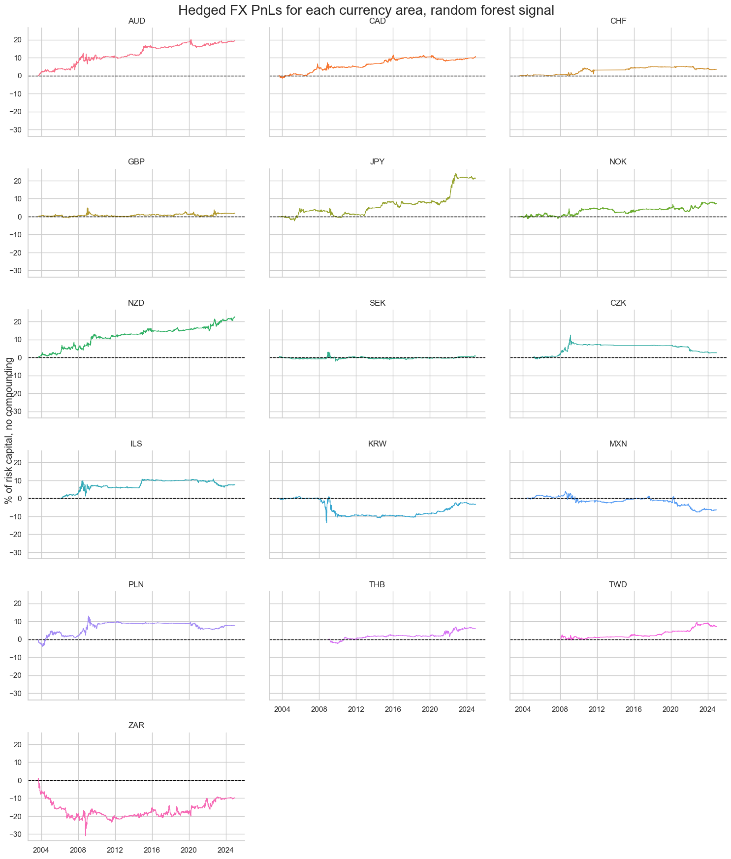
| cid | AUD | CAD | CHF | CZK | GBP | ILS | JPY | KRW | MXN | NOK | NZD | PLN | SEK | THB | TWD | ZAR |
|---|---|---|---|---|---|---|---|---|---|---|---|---|---|---|---|---|
| Return % | 0.914134 | 0.500497 | 0.198047 | 0.160895 | 0.084854 | 0.402986 | 1.008701 | -0.153109 | -0.309631 | 0.339651 | 1.065441 | 0.354967 | 0.033853 | 0.372088 | 0.415826 | -0.462428 |
| St. Dev. % | 2.185229 | 1.605812 | 0.860307 | 1.464976 | 1.452942 | 1.98409 | 2.107353 | 2.711666 | 1.775893 | 1.662936 | 2.031713 | 2.017494 | 0.979363 | 1.056361 | 1.009289 | 3.967962 |
| Sharpe Ratio | 0.418324 | 0.311678 | 0.230205 | 0.109828 | 0.058402 | 0.203109 | 0.478658 | -0.056463 | -0.174352 | 0.204248 | 0.524405 | 0.175944 | 0.034566 | 0.352236 | 0.411999 | -0.11654 |
| Sortino Ratio | 0.599076 | 0.430168 | 0.372181 | 0.18357 | 0.083173 | 0.305251 | 0.684705 | -0.083776 | -0.250708 | 0.290343 | 0.778096 | 0.248668 | 0.049728 | 0.583566 | 0.678884 | -0.160722 |
| Max 21-Day Draw % | -4.458108 | -3.200651 | -1.956676 | -4.463537 | -3.35628 | -6.409828 | -2.231307 | -7.319215 | -3.470926 | -3.433432 | -2.840344 | -2.777292 | -2.904183 | -1.763307 | -2.089691 | -12.418258 |
| Max 6-Month Draw % | -5.954793 | -3.004945 | -2.376887 | -4.955997 | -3.887387 | -5.732091 | -4.644383 | -11.366033 | -4.931902 | -3.891563 | -3.874994 | -5.503784 | -3.397354 | -2.121334 | -2.261274 | -9.033691 |
| Peak to Trough Draw % | -6.145171 | -3.742913 | -3.393439 | -10.069927 | -5.075318 | -8.833061 | -5.374178 | -14.582551 | -11.696147 | -4.381968 | -4.609159 | -7.610126 | -5.175616 | -3.418658 | -3.001471 | -32.100931 |
| Top 5% Monthly PnL Share | 0.909814 | 1.20764 | 2.3932 | 5.141337 | 5.962226 | 2.651177 | 1.125075 | -5.44129 | -1.856367 | 2.132598 | 1.060932 | 2.472955 | 11.25977 | 1.953303 | 1.596115 | -3.063043 |
| USD_GB10YXR_NSA correl | -0.03272 | -0.032432 | -0.008826 | 0.085455 | 0.00486 | 0.031284 | -0.183631 | -0.009299 | -0.015709 | 0.013866 | -0.092184 | 0.016045 | 0.052612 | -0.036613 | 0.000053 | -0.025174 |
| EUR_FXXR_NSA correl | -0.16552 | -0.23948 | 0.054663 | -0.058671 | -0.101999 | 0.114717 | -0.245962 | 0.00816 | -0.009367 | -0.031542 | -0.06326 | -0.015122 | -0.0608 | -0.155909 | -0.051019 | -0.001058 |
| USD_EQXR_NSA correl | -0.0382 | -0.033676 | 0.019192 | -0.079868 | -0.018731 | 0.032018 | 0.019384 | 0.050104 | 0.016776 | -0.057228 | 0.055331 | -0.045742 | -0.068592 | 0.024063 | 0.000473 | 0.049462 |
| Traded Months | 257 | 257 | 257 | 257 | 257 | 257 | 257 | 257 | 257 | 257 | 257 | 257 | 257 | 257 | 257 | 257 |