Equity market timing: the value of consumption data #
This notebook illustrates the points discussed in the post “Equity market timing: the value of consumption data” available on the Macrosynergy website.
The dividend discount model suggests that stock prices are negatively related to expected real interest rates and positively to earnings growth. The economic position of households or consumers influences both. Consumer strength spurs demand and exerts price pressure, thus pushing up real policy rate expectations. Meanwhile, tight labor markets and high wage growth shift national income from capital to labor. This post calculates a point-in-time score of consumer strength for 16 countries over almost three decades based on excess private consumption growth, import trends, wage growth, unemployment rates, and employment gains. This consumer strength score and most of its constituents displayed highly significant negative predictive power with regard to equity index returns. Value generation in a simple equity timing model has been material, albeit concentrated on business cycles’ early and late stages.
This notebook provides the essential code required to replicate the analysis discussed in the post.
The notebook covers the three main parts:
-
Get Packages and JPMaQS Data: This section is responsible for installing and importing the necessary Python packages used throughout the analysis.
-
Transformations and Checks: In this part, the notebook performs calculations and transformations on the data to derive the relevant signals and targets used for the analysis, including normalisation or building simple linear composite indicators.
-
Value checks: This is the most critical section, where the notebook calculates and implements the simple trading strategy based on the hypothesis tested in the post. This section involves backtesting simple trading strategies. In particular, the post investigates the predictive relationship of consumer strength scores for a simple equity overlay strategy.
It is important to note that while the notebook covers a selection of indicators and strategies used for the post’s main findings, users can explore countless other possible indicators and approaches. Users can modify the code to test different hypotheses and strategies based on their research and ideas. Best of luck with your research!
Get packages and JPMaQS data #
# Run only if needed!
"""
%%capture
! pip install macrosynergy --upgrade"""
'\n%%capture\n! pip install macrosynergy --upgrade'
import numpy as np
import pandas as pd
import os

import macrosynergy.management as msm
import macrosynergy.panel as msp
import macrosynergy.signal as mss
import macrosynergy.pnl as msn
from macrosynergy.download import JPMaQSDownload

import warnings
warnings.simplefilter("ignore")
This notebook downloads selected indicators for the following cross-sections: AUD (Australian dollar), BRL (Brazilian real), CAD (Canadian dollar), CHF (Swiss franc), EUR (euro), GBP (British pound), INR (Indian rupee), JPY (Japanese yen), KRW (Korean won), MXN (Mexican peso), MYR (Malaysian ringgit), SGD(Singapore dollar), SEK (Swedish krona), THB(Thai baht), TRY (Turkish lira), TWD (Taiwanese dollar), USD (U.S. dollar), ZAR (South African rand). For convenience purposes, the cross-sections are collected in a few lists, such as Developed markets large currencies (“EUR”, “JPY”, “USD”), emerging markets (“BRL”, “INR”, “KRW”, “MXN”, “MYR”, “SGD”, “THB”, “TRY”, “TWD”, “ZAR”), etc.
# Equity cross section lists

cids_g3 = ["EUR", "JPY", "USD"]  # DM large curency areas
cids_dmes = ["AUD", "CAD", "CHF", "GBP", "SEK"]  # Smaller DM equity countries
cids_dmeq = cids_g3 + cids_dmes  # DM equity countries

cids_emeq = ["BRL", "INR", "KRW", "MXN", "MYR", "SGD", "THB", "TRY", "TWD", "ZAR"]
cids_eq = cids_dmeq + cids_emeq
cids_eqx = list(set(cids_eq) - set(["INR", "TRY"]))  # countries with data issues

# Default

cids = cids_eq  # default for data import
The description of each JPMaQS category is available under Macro quantamental academy , or JPMorgan Markets (password protected). For tickers used in this notebook, see Private consumption , Wage growth , Labor market dynamics , GDP growth , Demographic trends , Inflation targets , and Equity index future returns .
# Categories

main = [
    "RPCONS_SA_P1M1ML12_3MMA",
    "RPCONS_SA_P1Q1QL4",
    "IMPORTS_SA_P6M6ML6AR",
    "WAGES_NSA_P1M1ML12_3MMA",
    "WAGES_NSA_P1Q1QL4",
    "EMPL_NSA_P1M1ML12_3MMA",
    "EMPL_NSA_P1Q1QL4",
    "UNEMPLRATE_SA_3MMAv5YMA",

]

xtra = [
    "RGDP_SA_P1Q1QL4_20QMM",
    "INFTEFF_NSA",
    "WFORCE_NSA_P1Y1YL1_5YMM",
]
rets = [
    "EQXR_NSA",
    "EQXR_VT10",
]

xcats = main + xtra + rets

xtix = ["GLB_DRBXR_NSA"]

tickers = [cid + "_" + xcat for cid in cids for xcat in xcats] + xtix
print(f"Maximum number of tickers is {len(tickers)}")
Maximum number of tickers is 235
# Download series from J.P. Morgan DataQuery by tickers

start_date = "1990-01-01"

# Retrieve credentials

client_id: str = os.getenv("DQ_CLIENT_ID")
client_secret: str = os.getenv("DQ_CLIENT_SECRET")

# Download from DataQuery

with JPMaQSDownload(client_id=client_id, client_secret=client_secret) as downloader:
    df = downloader.download(
        tickers=tickers,
        start_date=start_date,
        metrics=["value",],
        suppress_warning=True,
        show_progress=True,
    )
Downloading data from JPMaQS.
Timestamp UTC:  2025-03-05 15:52:53
Connection successful!
Requesting data: 100%|██████████| 12/12 [00:02<00:00,  4.90it/s]
Downloading data: 100%|██████████| 12/12 [00:15<00:00,  1.32s/it]
Some expressions are missing from the downloaded data. Check logger output for complete list.
57 out of 235 expressions are missing. To download the catalogue of all available expressions and filter the unavailable expressions, set `get_catalogue=True` in the call to `JPMaQSDownload.download()`.
Some dates are missing from the downloaded data.
2 out of 9180 dates are missing.
The JPMaQS indicators we consider are downloaded using the J.P. Morgan Dataquery API interface within the
macrosynergy
package. This is done by specifying ticker strings, formed by appending an indicator category code
DB(JPMAQS,<cross_section>_<category>,<info>)
, where
value
giving the latest available values for the indicator
eop_lag
referring to days elapsed since the end of the observation period
mop_lag
referring to the number of days elapsed since the mean observation period
grade
denoting a grade of the observation, giving a metric of real-time information quality.
After instantiating the
JPMaQSDownload
class within the
macrosynergy.download
module, one can use the
download(tickers,start_date,metrics)
method to easily download the necessary data, where
tickers
is an array of ticker strings,
start_date
is the first collection date to be considered and
metrics
is an array comprising the times series information to be downloaded. For more information see
here
dfx = df.copy()
dfx.info()
<class 'pandas.core.frame.DataFrame'>
RangeIndex: 1331684 entries, 0 to 1331683
Data columns (total 4 columns):
 #   Column     Non-Null Count    Dtype
---  ------     --------------    -----
 0   real_date  1331684 non-null  datetime64[ns]
 1   cid        1331684 non-null  object
 2   xcat       1331684 non-null  object
 3   value      1331684 non-null  float64
dtypes: datetime64[ns](1), float64(1), object(2)
memory usage: 40.6+ MB
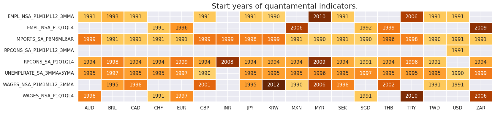
Availability #
It is important to assess data availability before conducting any analysis. It allows for the identification of any potential gaps or limitations in the dataset, which can impact the validity and reliability of analysis and ensure that a sufficient number of observations for each selected category and cross-section is available, as well as determining the appropriate time periods for analysis.
check_availability() functions list visualizes start years and the number of missing values at or before the end date of all selected cross-sections and across a list of categories. It also displays unavailable indicators as gray fields and color codes for the starting year of each series, with darker colors indicating more recent starting years.
The output below highlights the following:
-
Private consumption growth : most countries release quarterly data except for USA (USD) which produces a separate monthly-frequency data.
-
Employment growth : most countries release monthly-frequency data, but some countries, including Switzerland (CHF), the Eurozone (EUR), Mexico (MXN), Singapore (SGD), Thailand (THB) and South Africa (ZAR) only release quarterly data.
-
Wage growth : most countries in the selection release monthly data, apart from Australia (AUD), Switzerland (CHF), the Eurozone (EUR), Singapore (SGD), Turkey (TRY), and South Africa (ZAR).
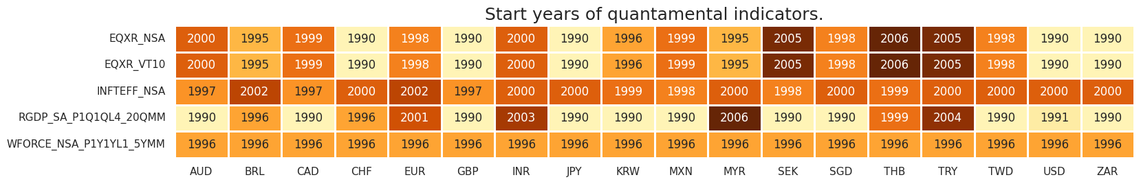
msm.check_availability(df, xcats=main, cids=cids, missing_recent=False)
msm.check_availability(df, xcats=xtra+rets, cids=cids, missing_recent=False)
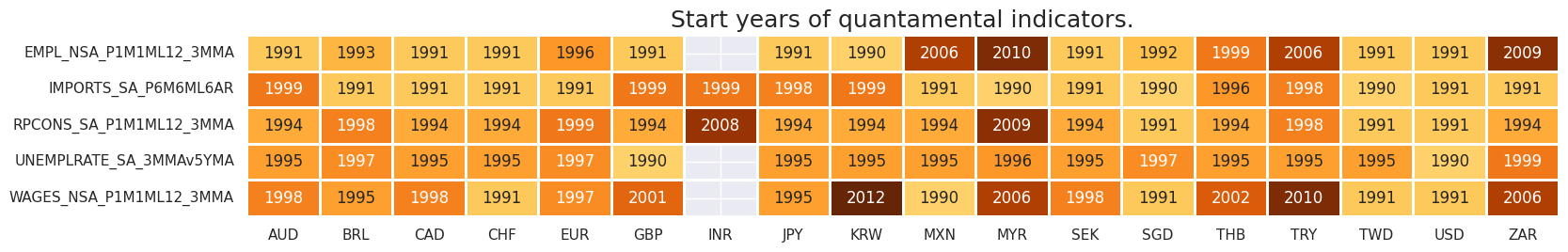
Rename categories #
Rename quarterly tickers to roughly equivalent monthly tickers to simplify subsequent operations ensuring that consistent indicators are available for all selected cross-sections.
dict_repl  = {
    "RPCONS_SA_P1Q1QL4": "RPCONS_SA_P1M1ML12_3MMA",
    "WAGES_NSA_P1Q1QL4": "WAGES_NSA_P1M1ML12_3MMA",
    "EMPL_NSA_P1Q1QL4": "EMPL_NSA_P1M1ML12_3MMA",
}

dfx['xcat'] = dfx['xcat'].replace(dict_repl)
Executing the check_availability() functions again verifies that the renaming process has successfully standardized the presence of consumption indicators throughout various segments of the dataset:
msm.check_availability(dfx, xcats=main, cids=cids, missing_recent=False)
Transformations and checks #
Features #
Here, we create five plausible indicators with complementary strengths that jointly give a good idea of consumer strength:
# Calculate logical excess trends

calcs = [
    "XRPCONS_SA_P1M1ML12_3MMA = RPCONS_SA_P1M1ML12_3MMA - RGDP_SA_P1Q1QL4_20QMM", # Excess consumption growth
    "XIMPORTS_SA_P6M6ML6AR = IMPORTS_SA_P6M6ML6AR - ( RGDP_SA_P1Q1QL4_20QMM + INFTEFF_NSA )", # Exces impport growth
    "XWAGES_NSA_P1M1ML12_3MMA = WAGES_NSA_P1M1ML12_3MMA - ( RGDP_SA_P1Q1QL4_20QMM - WFORCE_NSA_P1Y1YL1_5YMM + INFTEFF_NSA )", # Excess wage growth
    "XEMPL_NSA_P1M1ML12_3MMA = EMPL_NSA_P1M1ML12_3MMA - WFORCE_NSA_P1Y1YL1_5YMM", # Excess employment growth
]

dfa = msp.panel_calculator(dfx, calcs=calcs, cids=cids_eqx)
dfx = msm.update_df(dfx, dfa)
# For standardized directional theoretical impact changes sign of unemployment indicators

calcs = ["UNEMPLRATE_SA_3MMAv5YMAN = -1 * UNEMPLRATE_SA_3MMAv5YMA"]
dfa = msp.panel_calculator(dfx, calcs=calcs, cids=cids_eqx)
dfx = msm.update_df(dfx, dfa)
Normalized scores #
The process of standardizing the five indicators related to consumer spending and income prospects is achieved through the use of the
make_zn_scores()
function from the
macrosynergy
package. Normalization is a key step in macroeconomic analysis, especially when dealing with data across different categories that vary in units and time series characteristics. In this process, the indicators are centered around a neutral value (zero) using historical data. This normalization is recalculated monthly. To mitigate the impact of statistical outliers, a cutoff of 3 standard deviations is employed. Post-normalization, the indicators (z-scores) are labeled with the suffix
_ZNW3
, indicating their adjusted status.
alls = [
    "XRPCONS_SA_P1M1ML12_3MMA",
    "XIMPORTS_SA_P6M6ML6AR",
    "XWAGES_NSA_P1M1ML12_3MMA",
    "XEMPL_NSA_P1M1ML12_3MMA",
    "UNEMPLRATE_SA_3MMAv5YMAN",
]

dfa = pd.DataFrame(columns=dfx.columns)

for xc in alls:
    dfaa = msp.make_zn_scores(
        dfx,
        xcat=xc,
        cids=cids_eqx,
        sequential=True,
        min_obs=2 * 261,
        neutral="zero",
        pan_weight=1,
        thresh=3,
        postfix="_ZNW3",
        est_freq="M",
    )
    dfa = msm.update_df(dfa, dfaa)
dfx = msm.update_df(dfx, dfa)

allz = [x + "_ZNW3" for x in alls]
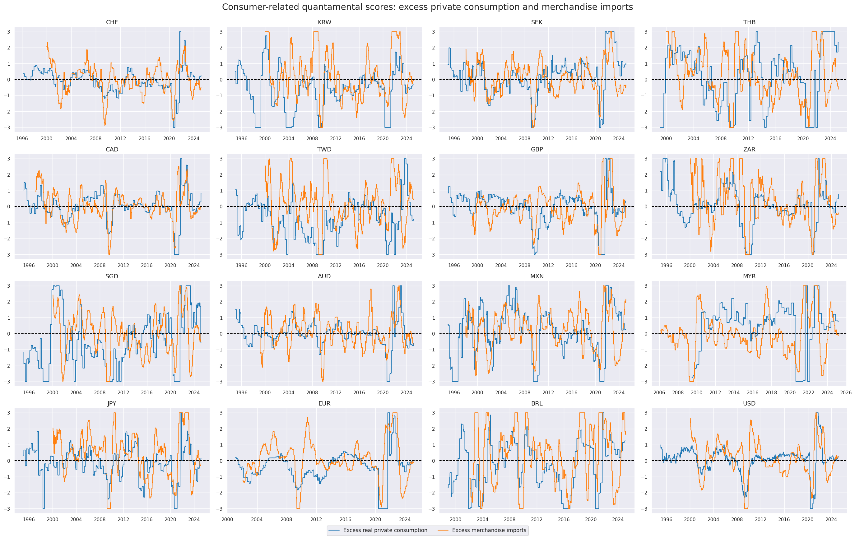
The z-scores of excess real private consumption and excess merchandise imports are displayed below with the help of
view_timelines()
from the
macrosynergy
package:
xcatx = allz[:2]
cidx = cids_eqx
sdate = "1995-01-01"

msp.view_timelines(
    dfx,
    xcats=xcatx,
    cids=cidx,
    ncol=4,
    cumsum=False,
    start=sdate,
    same_y=False,
    all_xticks=True,
    title="Consumer-related quantamental scores: excess private consumption and merchandise imports",
    title_fontsize=20,
    xcat_labels=["Excess real private consumption", "Excess merchandise imports"],
   )
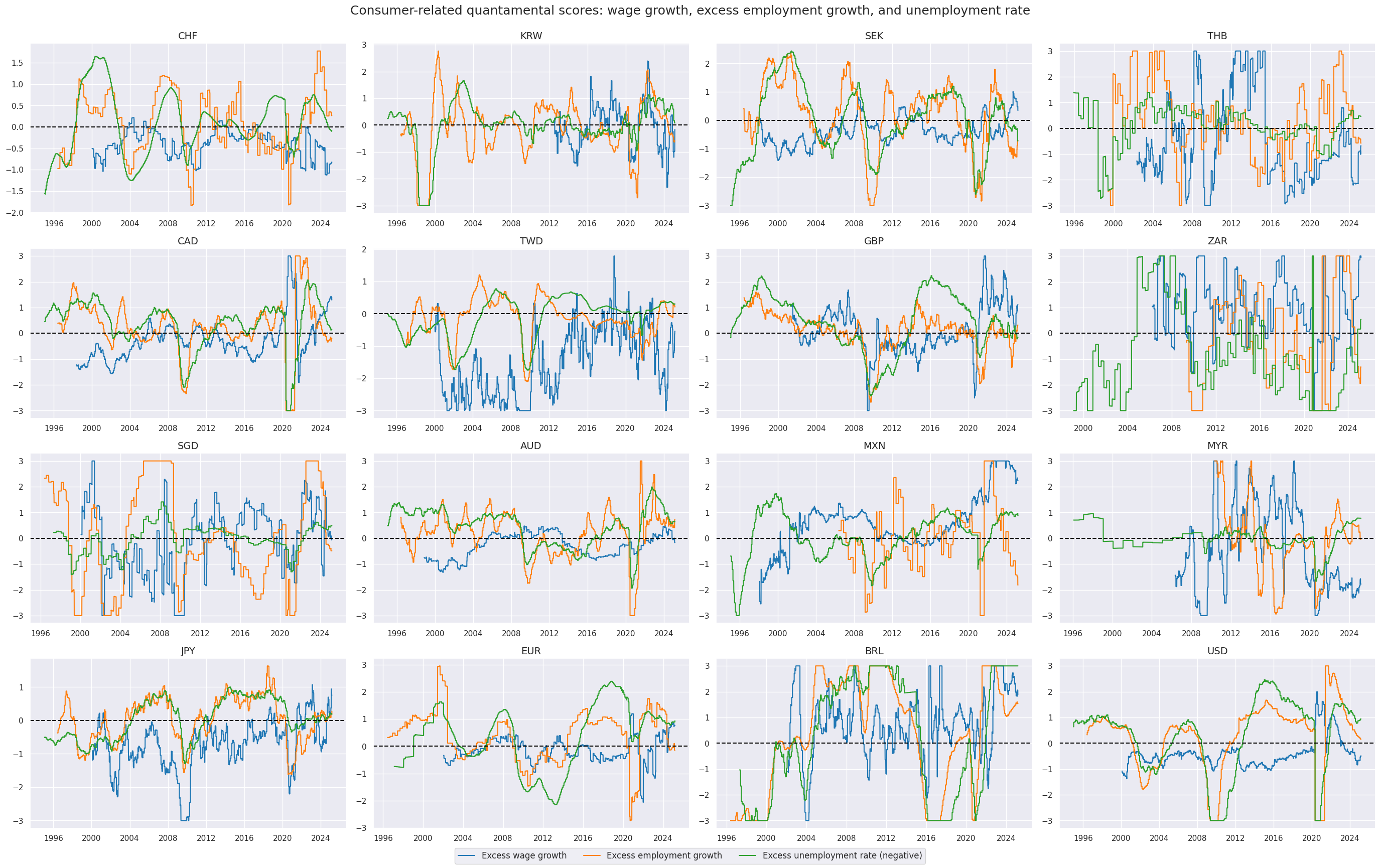
Labor-market related scores are displayed below:
xcatx = allz[2:]
cidx = cids_eqx
sdate = "1995-01-01"

msp.view_timelines(
    dfx,
    xcats=xcatx,
    cids=cidx,
    ncol=4,
    cumsum=False,
    start=sdate,
    same_y=False,
    all_xticks=True,
    title="Consumer-related quantamental scores: wage growth, excess employment growth, and unemployment rate",
    xcat_labels=["Excess wage growth", "Excess employment growth", "Excess unemployment rate (negative)"],

)
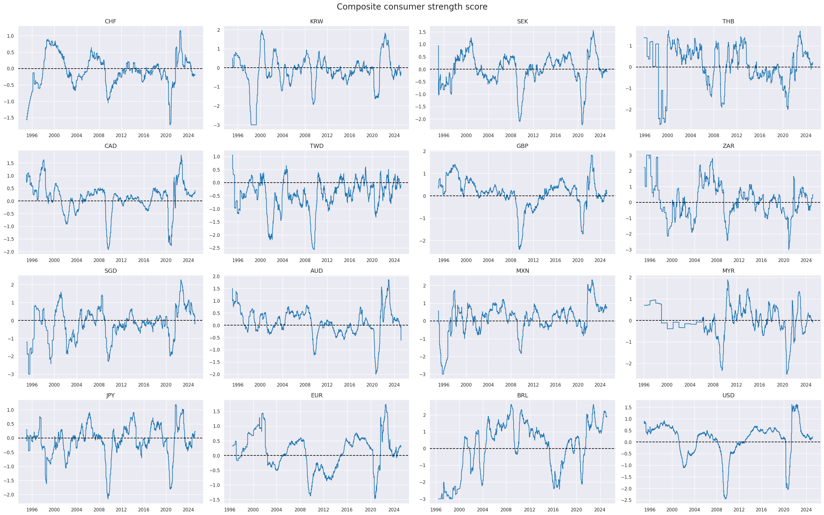
Composite score #
The
linear_composite
method from the
macrosynergy
package, as described in the Macrosynergy Academy’s documentation (Macrosynergy Academy), is employed to aggregate the individual category scores into a unified composite indicator. This method offers the flexibility to assign specific weights to each category, which can vary over time. In this instance, equal weights are applied to all categories, resulting in a composite indicator referred to as
ALL_CZN
. This approach ensures an even contribution from each category to the overall composite measure.
dfa = msp.linear_composite(
    dfx,
    xcats=allz,
    cids=cids_eqx,
    new_xcat = "ALL_CZN"
    )
dfx = msm.update_df(dfx, dfa)
ecoz = allz + ["ALL_CZN"]
view_timelines()
from the
macrosynergy
package is used to plot the timeline of the indicator across cross-sections:
xcatx = "ALL_CZN"
cidx = cids_eqx
sdate = "1995-01-01"

msp.view_timelines(
    dfx,
    xcats=xcatx,
    cids=cidx,
    ncol=4,
    cumsum=False,
    start=sdate,
    same_y=False,
    all_xticks=True,
    title="Composite consumer strength score",
    title_fontsize=20,
    )
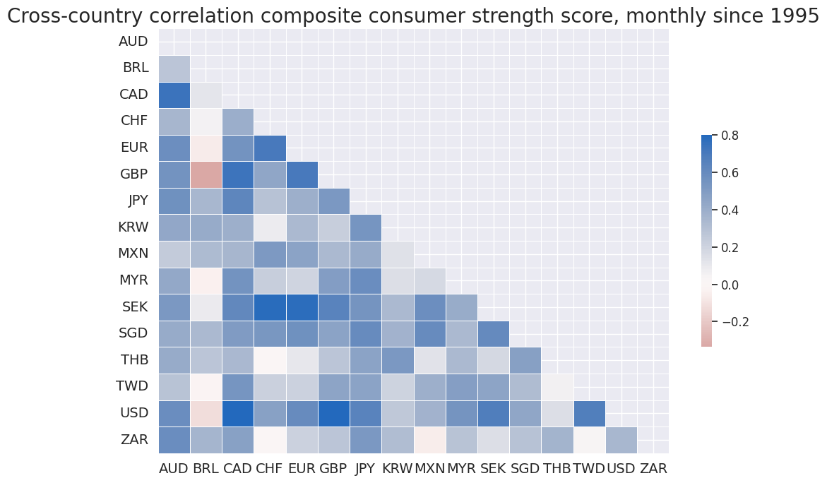
The function
correl_matrix()
of the
macrosynergy.panel
module allows to quickly visualize the historic international correlation of the signal category.
cidx = cids_eqx
msp.correl_matrix(
    dfx, xcats="ALL_CZN", freq="M", cids=cidx, start="1995-01-01", size=(10, 7), cluster=False,
    title="Cross-country correlation composite consumer strength score, monthly since 1995",
)
Targets #
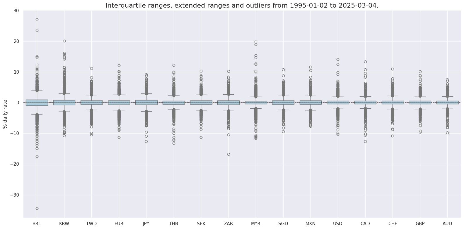
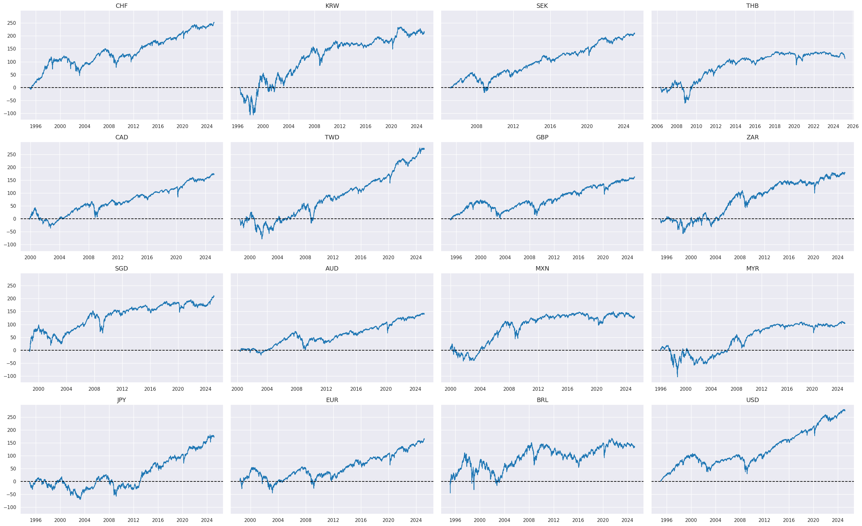
In this analysis, we use Equity index future returns in % of notional,
EQXR_NSA
, as our directional target. To effectively visualize the
EQXR_NSA
data across different countries, we utilize two helpful functions from the Macrosynergy package:
view_ranges()
and
view_timelines()
. The
view_ranges()
function is used for plotting the distributions of means and standard deviations, while
view_timelines()
is employed for illustrating the time series of these indicators, providing a comprehensive and clear visual representation of the data.
xcatx = ["EQXR_NSA"]
cidx = cids_eqx
sdate = "1995-01-01"

msp.view_ranges(
    dfx,
    cids=cidx,
    xcats=xcatx,
    kind="box",
    sort_cids_by="std",
    ylab="% daily rate",
    start=sdate,
)

msp.view_timelines(
    dfx,
    xcats=xcatx,
    cids=cidx,
    ncol=4,
    cumsum=True,
    start=sdate,
    same_y=True,
    all_xticks=True,

)
Value checks #
In this part of the analysis, the notebook calculates the naive PnLs (Profit and Loss) for Equity index future returns using individual consumer spending and income prospects indicators and the previously derived composite indicator. The PnLs are calculated based on simple trading strategies that utilize the indicators as signals (no regression is involved). The strategies involve going long (buying) or short (selling) on returns based purely on the direction of the score signals.
To evaluate the performance of these strategies, the notebook computes various metrics and ratios, including:
-
Correlation: Measures the relationship between indicator changes and consequent financial returns. Positive correlations indicate that the strategy moves in the same direction as the market, while negative correlations indicate an opposite movement.
-
Accuracy Metrics: These metrics assess the accuracy of the confidence score-based strategies in predicting market movements. Standard accuracy metrics include accuracy rate, balanced accuracy, precision, etc.
-
Performance Ratios: Various performance ratios, such as Sharpe ratio, Sortino ratio, Max draws, etc.
It’s important to note that the analysis deliberately disregards transaction costs and risk management considerations. This is done to provide a more straightforward comparison of the strategies’ raw performance without the additional complexity introduced by transaction costs and risk management, which can vary based on trading size, institutional rules, and regulations.
Specs and panel test #
feats = ecoz

targ = "EQXR_NSA"
cidx = cids_eqx
start = "1995-01-01"

dict_glb = {
    "sigs": feats,
    "sig": "ALL_CZN",
    "targ": targ,
    "cidx": cidx,
    "start": start,
    "srr": None,
    "pnls": None,
}
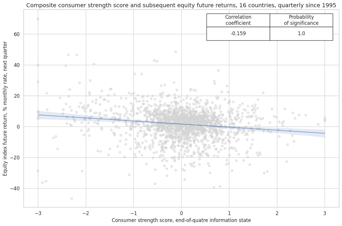
CategoryRelations()
function is used for quick visualization and analysis of two categories, in particular,
-
Composite consumer strength score
ALL_CZN, derived earlier, and -
subsequent equity future returns
EQXR_NSA.
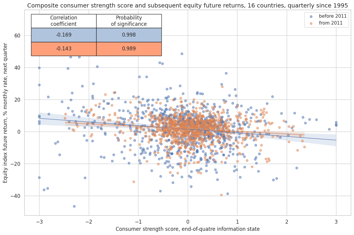
The
.reg_scatter()
method is convenient for visualizing the relationship between two categories, including the strength of the linear association and any potential outliers. It includes a regression line with a 95% confidence interval, which can help assess the significance of the relationship. The analysis is done on a quarterly basis. The same analysis is done for the whole available period and separately before and after 2011 to assess the stability of the relationship across time.
dix = dict_glb

sig = dix["sig"]
targ = dix["targ"]
cidx = dix["cidx"]
start = dix["start"]

crx = msp.CategoryRelations(
    dfx,
    xcats=[sig, targ],
    cids=cidx,
    freq="Q",
    lag=1,
    xcat_aggs=["last", "sum"],
    start=start,
    xcat_trims=[None, None],
)
crx.reg_scatter(
    labels=False,
    coef_box="upper right",
    title="Composite consumer strength score and subsequent equity future returns, 16 countries, quarterly since 1995",
    xlab="Consumer strength score, end-of-quatre information state",
    ylab="Equity index future return, % monthly rate, next quarter",
    size=(12, 8),
    prob_est="map"
)

crx.reg_scatter(
    labels=False,
    coef_box="upper left",
    title="Composite consumer strength score and subsequent equity future returns, 16 countries, quarterly since 1995",
    xlab="Consumer strength score, end-of-quatre information state",
    ylab="Equity index future return, % monthly rate, next quarter",
    size=(12, 8),
    prob_est="map",
    separator=2011,
)
Accuracy and correlation check #
The
SignalReturnRelations
class from the macrosynergy.signal module is designed to analyze, visualize, and compare the relationships between panels of trading signals and panels of subsequent returns.
dix = dict_glb

sigs = dix["sigs"]
targ = dix["targ"]
cidx = dix["cidx"]

srr = mss.SignalReturnRelations(
    dfx,
    cids=cidx,
    sigs=sigs,
    sig_neg=[True, True, True, True, True, True],
    rets=targ,
    freqs="M",
    start="2000-01-01",
)

dix["srr"] = srr
srrx = dix["srr"]
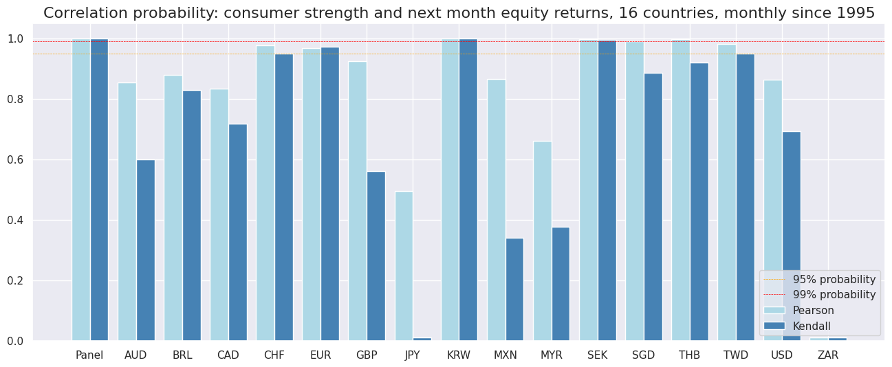
dix = dict_glb
srrx.correlation_bars(
    sigs="ALL_CZN",
    title="Correlation probability: consumer strength and next month equity returns, 16 countries, monthly since 1995",
    size=(16, 6)
)
display(srrx.multiple_relations_table().astype("float").round(3))
| accuracy | bal_accuracy | pos_sigr | pos_retr | pos_prec | neg_prec | pearson | pearson_pval | kendall | kendall_pval | auc | ||||
|---|---|---|---|---|---|---|---|---|---|---|---|---|---|---|
| Return | Signal | Frequency | Aggregation | |||||||||||
| EQXR_NSA | ALL_CZN_NEG | M | last | 0.507 | 0.511 | 0.474 | 0.583 | 0.594 | 0.428 | 0.110 | 0.000 | 0.047 | 0.000 | 0.511 |
| UNEMPLRATE_SA_3MMAv5YMAN_ZNW3_NEG | M | last | 0.487 | 0.500 | 0.421 | 0.583 | 0.583 | 0.417 | 0.058 | 0.000 | 0.031 | 0.002 | 0.500 | |
| XEMPL_NSA_P1M1ML12_3MMA_ZNW3_NEG | M | last | 0.500 | 0.511 | 0.436 | 0.582 | 0.594 | 0.427 | 0.072 | 0.000 | 0.030 | 0.003 | 0.511 | |
| XIMPORTS_SA_P6M6ML6AR_ZNW3_NEG | M | last | 0.506 | 0.513 | 0.460 | 0.585 | 0.600 | 0.427 | 0.095 | 0.000 | 0.034 | 0.001 | 0.514 | |
| XRPCONS_SA_P1M1ML12_3MMA_ZNW3_NEG | M | last | 0.510 | 0.510 | 0.502 | 0.584 | 0.593 | 0.426 | 0.084 | 0.000 | 0.040 | 0.000 | 0.510 | |
| XWAGES_NSA_P1M1ML12_3MMA_ZNW3_NEG | M | last | 0.525 | 0.504 | 0.620 | 0.587 | 0.590 | 0.417 | 0.037 | 0.014 | 0.008 | 0.432 | 0.504 |
Naive PnL #
The following dictionary provides user-friendly labels for both individual and composite consumer strength z-scores:
dict_labs = {
    "ALL_CZN": "Composite consumer strength score",
    "XRPCONS_SA_P1M1ML12_3MMA_ZNW3": "Excess real private consumption growth score",
    "XIMPORTS_SA_P6M6ML6AR_ZNW3": "Excess merchandise import growth score",
    "XWAGES_NSA_P1M1ML12_3MMA_ZNW3": "Excess wage growth score",
    "XEMPL_NSA_P1M1ML12_3MMA_ZNW3": "Excess employment growth score",
    "UNEMPLRATE_SA_3MMAv5YMAN_ZNW3": "Excess unemployment rate score",
}
Managed long #
NaivePnl()
class is designed to provide a quick and simple overview of a stylized PnL profile of a set of trading signals. The class is labeled naive because its methods do not consider transaction costs or position limitations, such as risk management considerations. This is deliberate because costs and limitations are specific to trading size, institutional rules, and regulations.
Important options within NaivePnl() function include:
-
zn_score_panoption transforms raw signals into z-scores around zero value based on the whole panel. The neutral level & standard deviation will use the cross-section of panels. zn-score here means standardized score with zero being the neutral level and standardization through division by mean absolute value. -
rebalancing frequency (
rebal_freq) for positions according to signal is chosen monthly, -
rebalancing slippage (
rebal_slip) in days is 1, which means that it takes one day to rebalance the position and that the new position produces PnL from the second day after the signal has been recorded, -
threshold value (
thresh) beyond which scores are winsorized, i.e., contained at that threshold. This is often realistic, as risk management and the potential of signal value distortions typically preclude outsized and concentrated positions within a strategy. We apply a threshold of 3. -
sig_add- this option creates a long-biased strategy, where 1 standard deviation for the long bias is added to the country score.
Long-only PnL is created with the label
               Long


               only
dix = dict_glb

sigx = dix["sigs"]
cidx = dix["cidx"]
targ = dix["targ"]
start = dix["start"]

naive_pnl = msn.NaivePnL(
    dfx,
    ret=targ,
    sigs=sigx,
    cids=cidx,
    start=start,
    bms=["USD_EQXR_NSA"],
)

for sig in sigx:
    naive_pnl.make_pnl(
        sig,
        sig_neg=True,
        sig_add=1,
        sig_op="zn_score_pan",
        thresh=3,
        rebal_freq="monthly",
        vol_scale=10,
        rebal_slip=1,
        pnl_name=sig + "_PZN",
    )

naive_pnl.make_long_pnl(vol_scale=10, label="Long only")
dix["pnls_ml"] = naive_pnl
The
plot_pnls()
method of the
NaivePnl()
class plots a line chart of cumulative PnL
The same method
plot_pnls()
of the
NaivePnl()
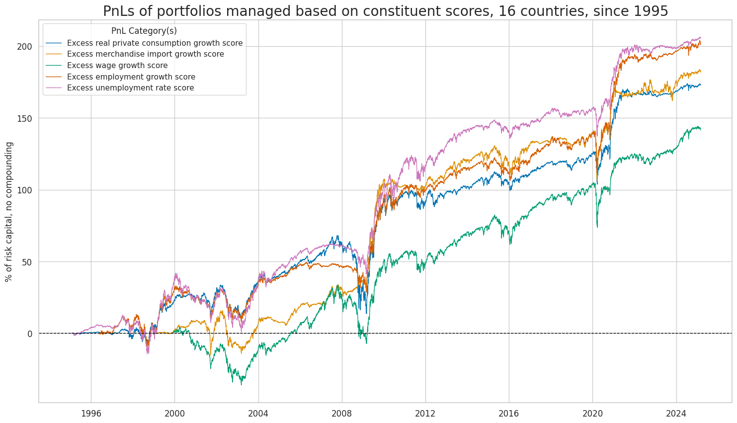
class can be used to plot a line chart of cumulative PnL for each of the five constituents of the composite consumer strength score.
dix = dict_glb
naive_pnl = dix["pnls_ml"]

start = dix["start"]
cidx = dix["cidx"]
sigx = dix["sigs"]
pnls = [s + "_PZN" for s in sigx if "ALL" not in s] #

new_keys = [x + "_PZN" for x in dict_labs.keys()]
dict_labx = {new_key: dict_labs[old_key] for new_key, old_key in zip(new_keys, dict_labs)}
labx = [dict_labx[x] for x in pnls]

naive_pnl.plot_pnls(
    pnl_cats=pnls,
    pnl_cids=["ALL"],
    start=start,
    title="PnLs of portfolios managed based on constituent scores, 16 countries, since 1995",
    xcat_labels=labx,
    figsize=(18, 10),
)
dix = dict_glb
naive_pnl = dix["pnls_ml"]

start = dix["start"]
sigx = dix["sigs"]
pnls = [sig + "_PZN" for sig in sigx] + ["Long only"]

df_eval = naive_pnl.evaluate_pnls(
    pnl_cats=pnls,
    pnl_cids=["ALL"],
    start=start
)
display(df_eval.transpose())
| Return % | St. Dev. % | Sharpe Ratio | Sortino Ratio | Max 21-Day Draw % | Max 6-Month Draw % | Peak to Trough Draw % | Top 5% Monthly PnL Share | USD_EQXR_NSA correl | Traded Months | |
|---|---|---|---|---|---|---|---|---|---|---|
| xcat | ||||||||||
| XRPCONS_SA_P1M1ML12_3MMA_ZNW3_PZN | 5.746219 | 10.0 | 0.574622 | 0.832716 | -30.029077 | -45.462352 | -54.558689 | 0.921452 | 0.509104 | 363 |
| XIMPORTS_SA_P6M6ML6AR_ZNW3_PZN | 6.953125 | 10.0 | 0.695313 | 1.08475 | -34.093228 | -29.982705 | -35.82187 | 0.917384 | 0.381973 | 363 |
| XWAGES_NSA_P1M1ML12_3MMA_ZNW3_PZN | 5.598326 | 10.0 | 0.559833 | 0.852863 | -29.546932 | -28.343951 | -40.768905 | 0.864386 | 0.554624 | 363 |
| XEMPL_NSA_P1M1ML12_3MMA_ZNW3_PZN | 6.986304 | 10.0 | 0.69863 | 1.030997 | -26.44476 | -23.138848 | -28.434665 | 0.821854 | 0.485288 | 363 |
| UNEMPLRATE_SA_3MMAv5YMAN_ZNW3_PZN | 6.812817 | 10.0 | 0.681282 | 0.976166 | -18.583233 | -26.961798 | -41.12412 | 0.821273 | 0.492516 | 363 |
| ALL_CZN_PZN | 7.495174 | 10.0 | 0.749517 | 1.095486 | -27.090622 | -28.642543 | -32.629871 | 0.823074 | 0.471819 | 363 |
| Long only | 4.783819 | 10.0 | 0.478382 | 0.660349 | -28.368634 | -44.578634 | -51.380704 | 0.79971 | 0.634963 | 363 |
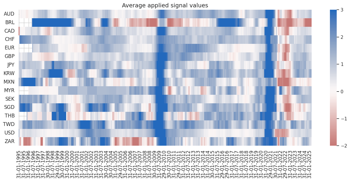
The
signal_heatmap
method creates a heatmap of signals for PnL across time and sections.
dix = dict_glb
naive_pnl = dix["pnls_ml"]

start = dix["start"]
sigx = [dix["sig"]]
pnls = sigx[0] + "_PZN"

naive_pnl.signal_heatmap(pnls, figsize=(16, 6))