Equity index future carry

The category group contains daily indicators of equity index carry. These are based on equity yields and local nominal or real funding costs. A currency area’s equity yield is estimated based on analysts’ dividends and earnings expectations for the most liquid available local index.

Nominal equity index carry

Ticker : EQCRY_NSA / EQCRY_VT10

Label : Nominal equity index future carry: % annualized / % annualized for 10% volatility target.

Definition : Estimated carry on main country equity index, based on the difference between (i) average of expected forward dividend and earnings yield and (ii) the main local-currency nominal short-term interest rate: % annualized of notional of the contract / % annualized of risk capital on position scaled to 10% (annualized) volatility target.

Notes :

• The index-related predicted dividend and earnings yields are based on forecasts of the IBES sample of analysts. Since both yields are used for carry calculation and there is no universally accepted convention, JPMaQS uses an average of the 12-month forward expectations of earnings and dividend yields. We call this average the “equity yield”.

• The nominal carry is the equity yield minus the local 1-month interbank or OIS rate or its closest proxy.

• For volatility targeting, positions are scaled to 10% vol-target based on historic standard deviation for an exponential moving average with a half-life of 11 days. Positions are rebalanced at the end of each month.

• See Appendix 1 for the list of equity indicies used for each currency area.

Alternative nominal equity index carry

Ticker : EQNASDAQCRY_NSA / EQRUSSELLCRY_NSA / EQTOPIXCRY_NSA / EQHANGSENGCRY_NSA / EQNASDAQCRY_VT10 / EQRUSSELLCRY_VT10 / EQTOPIXCRY_VT10 / EQHANGSENGCRY_VT10

Label : Nominal equity index future carry: % annualized NASDAQ 100 / % annualized Russell 2000 / % annualized TOPIX / % annualized Hang Seng / % annualized for 10% volatility target NASDAQ 100 / % annualized for 10% volatility target Russell 2000 / % annualized for 10% volatility target TOPIX / % annualized for 10% volatility target Hang Seng.

Definition : Estimated carry on alternative country equity index, based on the difference between (i) average of expected forward dividend and earnings yield and (ii) the main local-currency nominal short-term interest rate: % annualized of notional of the contract (NASDAQ 100) / % annualized of notional of the contract (RUSSELL 2000) / % annualized of notional of the contract (TOPIX) / % annualized of notional of the contract (HANG SENG) / % annualized of risk capital on position scaled to 10% (annualized) volatility target (NASDAQ 100) / % annualized of risk capital on position scaled to 10% (annualized) volatility target (RUSSELL 2000) / % annualized of risk capital on position scaled to 10% (annualized) volatility target (TOPIX) / % annualized of risk capital on position scaled to 10% (annualized) volatility target (HANG SENG).

Notes :

• Alternative indices are not the main equity index of the country but are available for suplementary analyses.

• See Appendix 2 for the list of alternative equity indices used. Alternative indices are available for HKD, JPY, and USD.

• See the important notes under “Nominal equity index carry” ( EQCRY_NSA ).

Real equity index carry

Ticker : EQCRR_NSA / EQCRR_VT10

Label : Real equity index future carry: % annualized / % annualized for 10% volatility target.

Definition : Estimated carry on main country equity index, based on the difference between (i) average of expected forward dividend and earnings yield and (ii) the main local-currency real short-term interest rate: % annualized of notional of the contract / % annualized of risk capital on position scaled to 10% (annualized) volatility target.

Notes :

• Real carry means that the conventional (nominal) carry is adjusted for the effect of expected inflation. Since high inflation does not conceptually reduce the equity yield, which is calculated on the basis of a real asset, but does reduce funding costs, which is calculated on the basis of a nominal liability, it is the only funding cost proxy that must be adjusted. Hence, rather than using a nominal interest rate, this carry indicator uses a real interest rate.

• The real interest rate is the main local 1-month interbank or OIS rate, or closest proxy, minus inflation expectation. The latter are the 1-year ahead estimated inflation expectations according to Macrosynergy methodology.

• See the notes on INFE1Y_JA in “Inflation expectations (Macrosynergy methodology)”.

Alternative real equity index carry

Ticker : EQNASDAQCRR_NSA / EQRUSSELLCRR_NSA / EQTOPIXCRR_NSA / EQHANGSENGCRR_NSA / EQNASDAQCRR_VT10 / EQRUSSELLCRR_VT10 / EQTOPIXCRR_VT10 / EQHANGSENGCRR_VT10

Label : Real equity index future carry: % annualized NASDAQ 100 / % annualized Russell 2000 / % annualized TOPIX / % annualized Hang Seng / % annualized for 10% volatility target NASDAQ 100 / % annualized for 10% volatility target Russell 2000 / % annualized for 10% volatility target TOPIX / % annualized for 10% volatility target Hang Seng.

Definition : Estimated carry on alternative country equity index, based on the difference between (i) average of expected forward dividend and earnings yield and (ii) the main local-currency real short-term interest rate: % annualized of notional of the contract (NASDAQ 100) / % annualized of notional of the contract (RUSSELL 2000) / % annualized of notional of the contract (TOPIX) / % annualized of notional of the contract (HANG SENG) / % annualized of risk capital on position scaled to 10% (annualized) volatility target (NASDAQ 100) / % annualized of risk capital on position scaled to 10% (annualized) volatility target (RUSSELL 2000) / % annualized of risk capital on position scaled to 10% (annualized) volatility target (TOPIX) / % annualized of risk capital on position scaled to 10% (annualized) volatility target (HANG SENG).

Notes :

• Alternative indices are not the main equity index of the country but are available for suplementary analyses.

• See Appendix 2 for the list of alternative equity indices used. Alternative indices are available for HKD, JPY, and USD.

• See the important notes under “Real equity index carry” ( EQCRR_NSA ).

Imports

Only the standard Python data science packages and the specialized macrosynergy package are needed.

import os
import pandas as pd

import macrosynergy.management as msm
import macrosynergy.panel as msp
import macrosynergy.signal as mss
import macrosynergy.visuals as msv

from macrosynergy.download import JPMaQSDownload

from timeit import default_timer as timer
from datetime import timedelta, date

import warnings

warnings.simplefilter("ignore")

The JPMaQS indicators we consider are downloaded using the J.P. Morgan Dataquery API interface within the macrosynergy package. This is done by specifying ticker strings , formed by appending an indicator category code <category> to a currency area code <cross_section> . These constitute the main part of a full quantamental indicator ticker, taking the form DB(JPMAQS,<cross_section>_<category>,<info>) , where <info> denotes the time series of information for the given cross-section and category. The following types of information are available:

• value giving the latest available values for the indicator

• eop_lag referring to days elapsed since the end of the observation period

• mop_lag referring to the number of days elapsed since the mean observation period

• grade denoting a grade of the observation, giving a metric of real time information quality.

After instantiating the JPMaQSDownload class within the macrosynergy.download module, one can use the download(tickers,start_date,metrics) method to easily download the necessary data, where tickers is an array of ticker strings, start_date is the first collection date to be considered and metrics is an array comprising the times series information to be downloaded.

# Cross-sections of interest

cids_dmeq = ['AUD', 'CAD', 'CHF', 'EUR', 'GBP', 'JPY', 'SEK', 'USD'] # NOK and NZD not available
cids_eueq = ["DEM", "ESP", "FRF", "ITL", "NLG"]
cids_aseq = ["CNY", "HKD", "INR", "KRW", "MYR", "SGD", "THB", "TWD"]
cids_exeq = ["BRL", "TRY", "ZAR"]
cids_nueq = ["MXN", "PLN"]
cids_emeq = list(set(cids_aseq + cids_exeq + cids_nueq)) # 'HKD', "ILS" not available

# For FX analyses

cids_nofx = ["USD", "EUR", "CNY", "SGD"]
cids_fx = list(set(cids_dmeq + cids_emeq) - set(cids_nofx))
cids_dmfx = list(set(cids_dmeq) - set(cids_nofx))
cids_emfx = list(set(cids_emeq) - set(cids_nofx))

cids_eur = ["CHF", "NOK", "SEK", "PLN", "HUF", "CZK"]  # trading against EUR
cids_eud = ["GBP"]  # trading against EUR and USD
cids_usd = list(set(cids_fx) - set(cids_eur + cids_eud))  # trading against USD


cids = sorted(cids_dmeq + cids_eueq + cids_aseq + cids_exeq + cids_nueq)

main = ["EQCRR_NSA", "EQCRR_VT10", "EQCRY_NSA", "EQCRY_VT10"]

econ = ["FXTARGETED_NSA",
    "FXUNTRADABLE_NSA",]  # economic context

mark = [
    "EQXR_NSA",
    "EQXR_VT10",
    "FXCRY_NSA", 
    "FXXR_VT10",
    "FXXR_NSA",
  ]  # market links

xcats = main + econ + mark

tickers = [cid + "_" + xcat for cid in cids for xcat in xcats]

# For alternative indices - Russell, Nasdaq, Topix, Hang Seng:

alt_markets = {
    "USD": ["EQNASDAQ", "EQRUSSELL"],
    "JPY": ["EQTOPIX"],
    "HKD": ["EQHANGSENG"]
}

suffixes = ["CRY_NSA", "XR_NSA", "CRY_VT10", "CRR_NSA", "CRR_VT10"]

alt_tickers = [
    f"{cid}_{market}{suffix}"
    for cid, markets in alt_markets.items()
    for market in markets
    for suffix in suffixes
]


tickers.extend(alt_tickers)
print(f"Maximum number of tickers is {len(tickers)}")

Maximum number of tickers is 306

# Download series from J.P. Morgan DataQuery by tickers

start_date = "2000-01-01"

# Retrieve credentials

client_id: str = os.getenv("DQ_CLIENT_ID")
client_secret: str = os.getenv("DQ_CLIENT_SECRET")

# Download from DataQuery

with JPMaQSDownload(client_id=client_id, client_secret=client_secret) as downloader:
    start = timer()
    assert downloader.check_connection()
    df = downloader.download(
        tickers=tickers,
        start_date=start_date,
        metrics=["value", "eop_lag", "mop_lag", "grading"],
        suppress_warning=True,
        show_progress=True,
    )
    end = timer()


print("Download time from DQ: " + str(timedelta(seconds=end - start)))

Downloading data from JPMaQS.
Timestamp UTC:  2025-03-06 15:55:52
Connection successful!

Requesting data: 100%|██████████| 62/62 [00:12<00:00,  4.86it/s]
Downloading data: 100%|██████████| 62/62 [00:38<00:00,  1.61it/s]

Some expressions are missing from the downloaded data. Check logger output for complete list.
132 out of 1224 expressions are missing. To download the catalogue of all available expressions and filter the unavailable expressions, set `get_catalogue=True` in the call to `JPMaQSDownload.download()`.
Download time from DQ: 0:00:56.889839

Availability

cids_exp = cids  # cids expected in category panels
msm.missing_in_df(df, xcats=main, cids=cids_exp)

No missing XCATs across DataFrame.
Missing cids for EQCRR_NSA:   []
Missing cids for EQCRR_VT10:  []
Missing cids for EQCRY_NSA:   []
Missing cids for EQCRY_VT10:  []

Quantamental indicators for equity index future carry are typically available, for developed markets, by the early 2000s. Many emerging markets only have data available from 2004 onwards.

For the explanation of currency symbols, which are related to currency areas or countries for which categories are available, please view Appendix 3 .

xcatx = main
cidx = cids_exp

dfx = msm.reduce_df(df, xcats=xcatx, cids=cidx)
dfs = msm.check_startyears(
    dfx,
)
msm.visual_paneldates(dfs, size=(18, 4))

print("Last updated:", date.today())

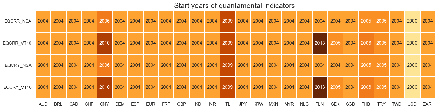
Last updated: 2025-03-06

Alternative indicators are available for HKD, JPY and USD. They enable suplementary analyses with different focuses when compared to the country’s main index (small caps, broader/narrower coverage, etc.). Quantamental indicators for equity index future carry are avaible since 2004 for most alternative indices, with the expection of NASDAQ 100 that starts in 2010.

suffixes = ["CRY_NSA", "CRY_VT10", "CRR_NSA", "CRR_VT10"]
alt_cats = [f"{market}{suffix}" for markets in alt_markets.values() for market in markets for suffix in suffixes]

# Define relevant currencies
cidx = list(alt_markets.keys())

# Check and validate start years
dfaa = msm.reduce_df(df, xcats=alt_cats, cids=cidx)
dfs = msm.check_startyears(
    dfaa,
)

# Creating the dataframe for alternative indices
dfs_alt = pd.DataFrame(
    [
        {
            f"{index}_{col}": dfs.loc[index, col]
            for index in dfs.index
            for col in dfs.columns
            if not pd.isna(dfs.loc[index, col])
        }
    ]
)
dfs_alt["idx"] = ""
dfs_alt = dfs_alt.set_index("idx")

msm.visual_paneldates(dfs_alt, size=(6, 4))

print("Last updated:", date.today())

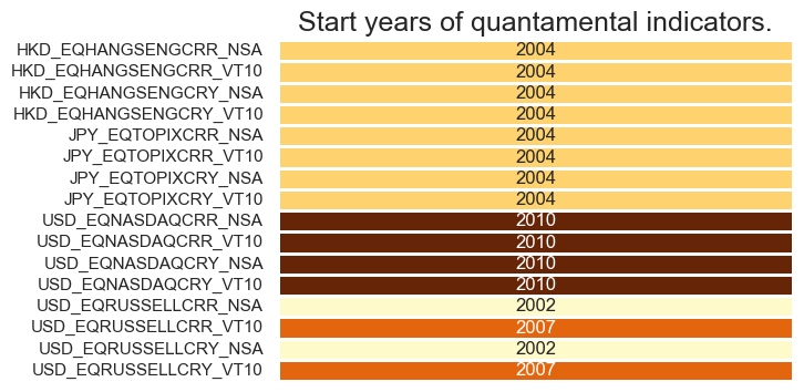
Last updated: 2025-03-06

History

Equity carry in % of notional

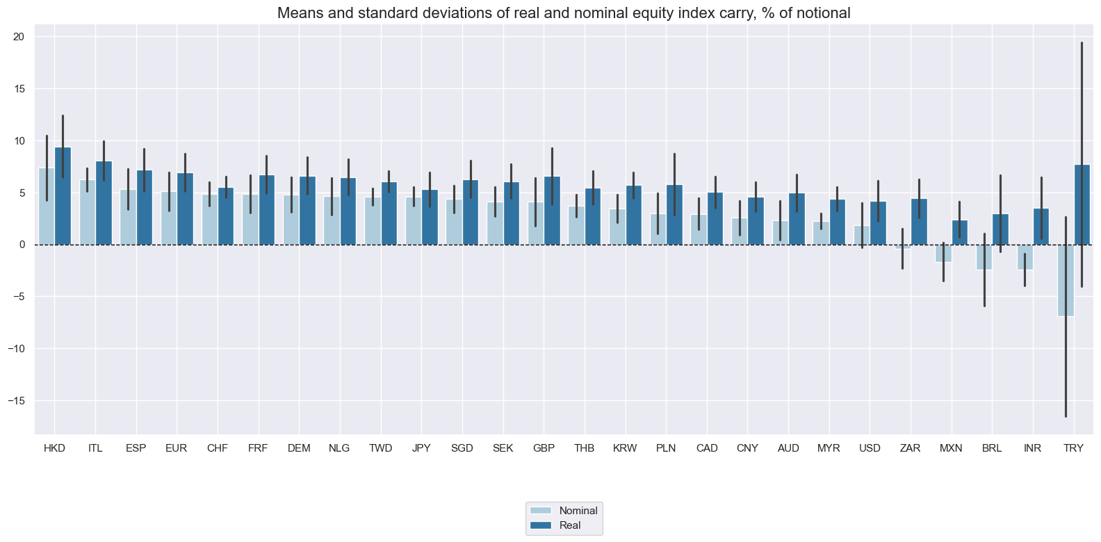
There have been large differences in real and nominal carry. Naturally, the nominal measure in high-inflation markets would have massively underestimated the real carry on a funded equity derivative. This illustrates that standard nominal equity carry can be misleading.

The importance of inflation suggests that real carry measures are economically more meaningful, even if there can be signficant estimation errors in real-time inflation expectations. Real carry measures are more even and comparable across countries.

xcatx = ["EQCRY_NSA", "EQCRR_NSA"]
cidx = cids_exp

msp.view_ranges(
    df,
    xcats=xcatx,
    cids=cidx,
    sort_cids_by="mean",
    start="2000-01-01",
    kind="bar",
    title="Means and standard deviations of real and nominal equity index carry, % of notional",
    xcat_labels=["Nominal", "Real"],
    size=(16, 8),
)

xcatx = ["EQCRY_NSA", "EQCRR_NSA"]
cidx = cids_exp

lab_dict = {
    "EQCRR_NSA": "Real equity index future carry: % ann",
    "EQCRY_NSA": "Nominal equity index future carry: % ann", 
   }
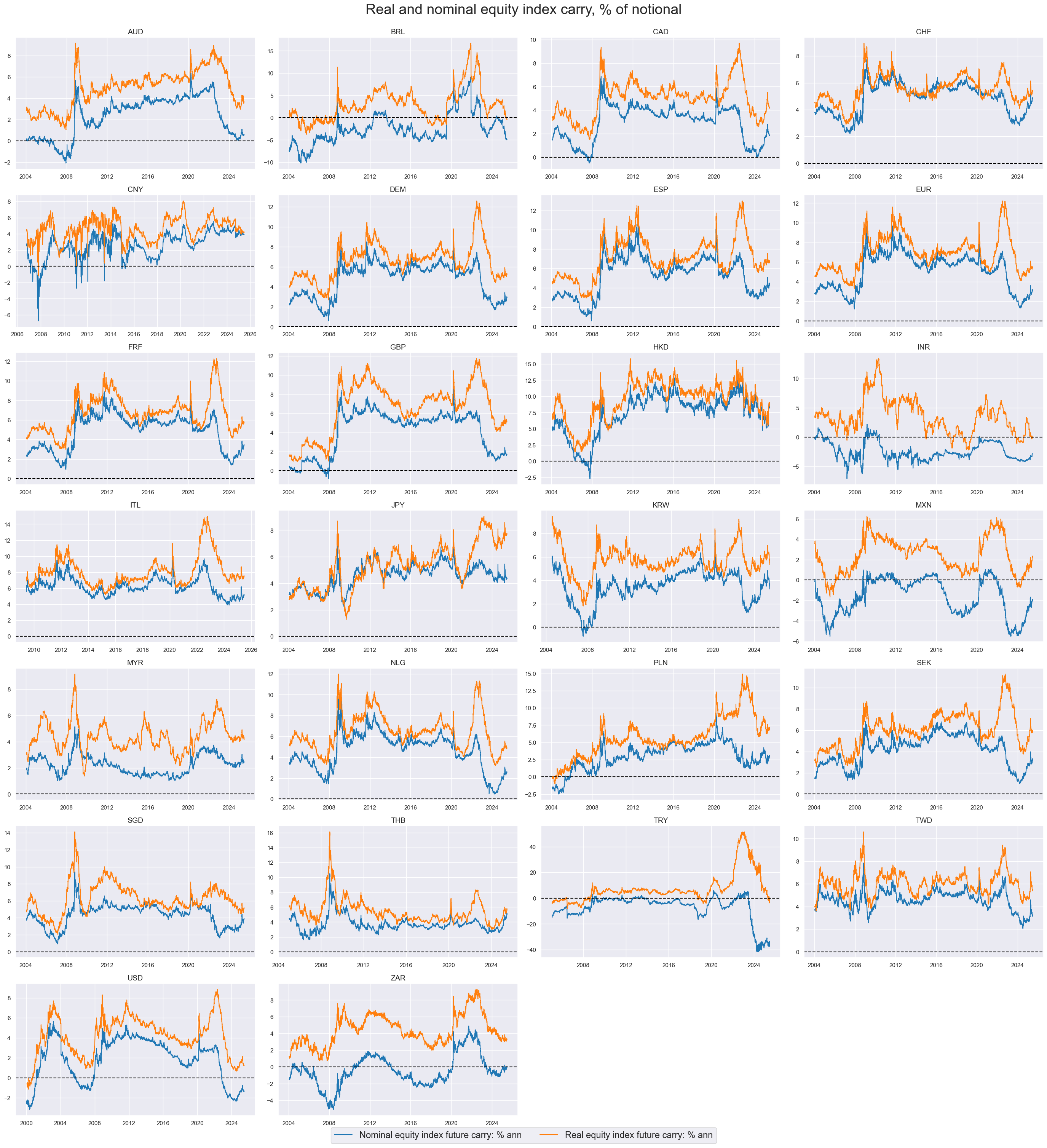
msp.view_timelines(
    df,
    xcats=xcatx,
    cids=cidx,
    start="2000-01-01",
    title="Real and nominal equity index carry, % of notional",
    title_fontsize=27,
    legend_fontsize=17,
    xcat_labels=lab_dict,
    ncol=4,
    same_y=False,
    size=(12, 7),
    all_xticks=True,
)

Despite their similarities, alternative indices provide a different lens to evaluate the market, revealing distinct return dynamics throughout history - such as the increase in the gap between the carry of Hang Seng China Enterprises vs Hang Seng after 2010.

lab_dict = {
    "EQCRY_NSA": "Nominal equity index future carry: % ann", 
    "EQRUSSELLCRY_NSA": "Nominal equity index future carry: % ann Russell 2000", 
    "EQNASDAQCRY_NSA": "Nominal equity index future carry: % ann NASDAQ 100", 
    "EQTOPIXCRY_NSA": "Nominal equity index future carry: % ann TOPIX", 
    "EQHANGSENGCRY_NSA": "Nominal equity index future carry: % ann Hang Seng",  
}



msp.view_timelines(
    df,
    xcats=["EQCRY_NSA", "EQNASDAQCRY_NSA", "EQRUSSELLCRY_NSA", "EQHANGSENGCRY_NSA", "EQTOPIXCRY_NSA"],
    cids=['HKD', 'JPY', 'USD'],
    start="2000-01-01",
    title="Nominal equity index carry on main local-currency equity index vs alternative index",
    title_fontsize=27,
    legend_fontsize=17,
    ncol=4,
    same_y=False,
    xcat_labels=lab_dict,
    size=(12, 7),
    aspect=1.5,
    all_xticks=True,
)

Cross-country correlations of real equity have been mostly postive since since 2000.

xcatx = "EQCRR_NSA"
cidx = cids_exp

msp.correl_matrix(
    df,
    xcats=xcatx,
    cids=cidx,
    title="Cross-sectional correlations of real equity index future carry, since 2000",
    size=(20, 14),
)

Vol-targeted equity index carry

Vol-targeted real equity carry has typically averaged 1%-5% across countries. Due to the combination of fast volatility-adjustment and sluggish equity yield revisions, the indicator has a lot more short-term variability than non-targeted carry. That volatility is all driven by recent market price fluctuations.

xcatx = ["EQCRY_VT10", "EQCRR_VT10"]
cidx = cids_exp

msp.view_ranges(
    df,
    xcats=xcatx,
    cids=cidx,
    sort_cids_by="mean",
    start="2000-01-01",
    kind="bar",
    title="Means and standard deviations of real and nominal equity index carry, % of notional, 10% vol-target",
    xcat_labels=["Nominal", "Real"],
    size=(16, 8),
)

xcatx = ["EQCRY_VT10", "EQCRR_VT10"]
cidx = cids_exp
lab_dict = {
    "EQCRR_VT10": "Real equity index future carry: % ann for 10% vol target",
    "EQCRY_VT10": "Nominal equity index future carry: % ann for 10% vol target",
 }



msp.view_timelines(
    df,
    xcats=xcatx,
    cids=cidx,
    start="2000-01-01",
    title="Real and nominal equity index carry, % of notional, 10% vol-targeting",
    title_fontsize=27,
    legend_fontsize=17,
    ncol=4,
    xcat_labels=lab_dict,
    same_y=True,
    size=(12, 7),
    all_xticks=True,
)

Importance

Research Links

“Forward earnings yields and equity carry are plausible indicators of risk premia embedded in equity index futures prices. Data for a panel of 25 developed and emerging markets from 2000 to 2018 show that index forward earnings yields have been correlated with market uncertainty across countries and time. Earnings yields have been highest in emerging countries. However, equity carries have not, because they depend on local funding conditions and only indicate the country risk premium that is specific to equity. Both yield and carry metrics display convincing and consistent positive correlation with subsequent index futures returns. Simulations show that for proper equity long-short strategies active volatility adjustment of both signals and positions is essential in order to balance risk premia with the actual state of riskiness of the market.” Macrosynergy

“Forward earnings yields are a key metric for the valuation of an equity market. Helpfully, I/B/E/S and DataStream publish forward earnings forecasts of analysts on a market-wide index basis. Unfortunately, updates of these data are delayed by multiple lags. This can make them inaccurate and misleading in times of rapidly changing macroeconomic conditions. Indeed, there is strong empirical evidence that equity index price changes predict future forward earnings revisions significantly and for all of the world’s 25 most liquid local equity markets. This predictability can be used to enhance the precision of real-time earnings yield data and avoid misleading trading signals.” Macrosynergy

“The results … indicate that carry is a strong predictor of expected returns, with consistently positive and statistically significant coefficients on carry, save for the commodity strategy, which can be tainted by strong seasonal effects in carry for commodities, and for call options.” “carry produces different and stronger return predictability than the standard predictor in all asset classes except for commodities and currencies, when they are the same” R Koijen, T Moskowitz, L Pedersen, E Vrugt

“We thus suggested that … evidence, in support of a depreciation of the German mark subsequent to the outperformance of the German over the US stock market, may not be due to risk aversion of investors but rather to carry trades,… that have a seasonal character ignored in the existing literature.” E Girardin, F Salimi Namin

“Carry strategies have become one of the main pillars of risk-premia investing.” D Tzotchev

Empirical Clues

Equity index carry and subsequent returns

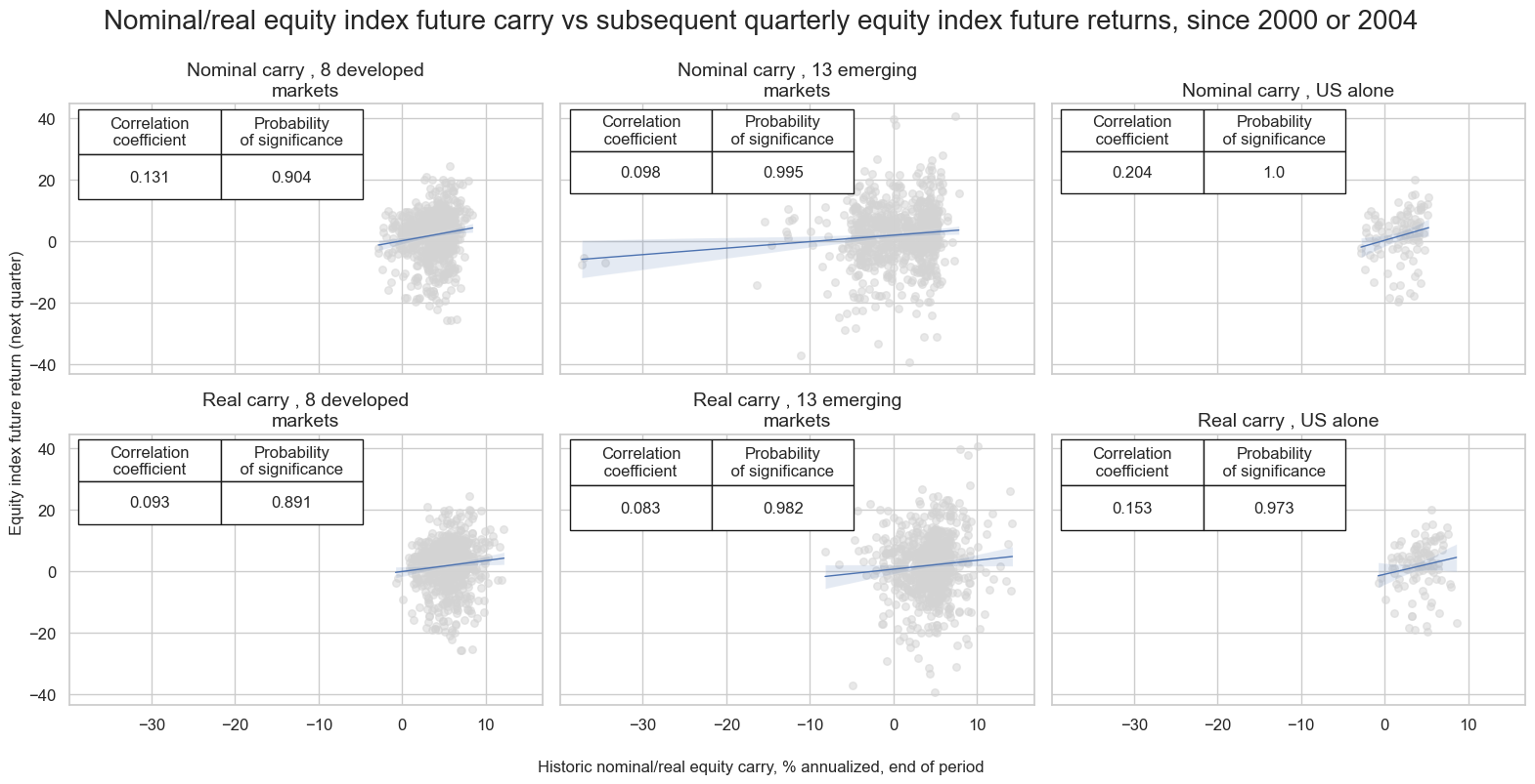
All other things equal, a higher equity index carry should herald higher medium-term returns. Carry indicates intertemporal and cross-country risk premia. In practice this relation is diluted by structural difference across country equity indices in companies, sectors, taxation, and regulatory rules. Indeed, there is pervasive evidence of a positive correlation between equity index carry and subsequent returns for both developed and emerging markets on quarterly, monthly and weekly frequency. The relationship has been particularly strong and significant for the U.S. market.

# U.S. FX market restrictions for blacklisting

dfx = df.copy()

dfb = dfx[dfx["xcat"].isin(["FXTARGETED_NSA", "FXUNTRADABLE_NSA"])].loc[
    :, ["cid", "xcat", "real_date", "value"]
]
dfba = (
    dfb.groupby(["cid", "real_date"])
    .aggregate(value=pd.NamedAgg(column="value", aggfunc="max"))
    .reset_index()
)
dfba["xcat"] = "FXBLACK"
fxblack = msp.make_blacklist(dfba, "FXBLACK")

# Define signal and target dictionaries
sigx_dict_eq = {
    "EQCRY_NSA": "Nominal carry",
    "EQCRR_NSA": "Real carry", 
}

targx_dict_eq = {
    "EQXR_NSA": "equity index future return",
}

cidx_dict_eq = {
    f"{len(set(cids_dmeq))} developed markets": list(set(cids_dmeq)),  # DM separate
    f"{len(set(cids_emeq))} emerging markets": list(set(cids_emeq)),  # EM separate
    "US alone": ["USD"],  # US gets its own row
}

# Create CategoryRelations instances
cr = {}

for cid_name, cid_list in cidx_dict_eq.items():
    for sig_name in sigx_dict_eq.keys():
        cr[f"cr_{sig_name}_{cid_name}"] = msp.CategoryRelations(
            dfx,
            xcats=[sig_name] + list(targx_dict_eq.keys()),  
            cids=cid_list,  
            freq="q",
            blacklist=fxblack,
            lag=1,
            xcat_aggs=["last", "sum"],
            start="2000-01-01",
        )

# Define the correct order for rows

row_order = [
    [("EQCRY_NSA", f"{len(set(cids_dmeq))} developed markets"), ("EQCRY_NSA", f"{len(set(cids_emeq))} emerging markets"), ("EQCRY_NSA", "US alone")],  
    [("EQCRR_NSA", f"{len(set(cids_dmeq))} developed markets"), ("EQCRR_NSA", f"{len(set(cids_emeq))} emerging markets"), ("EQCRR_NSA", "US alone")],     
]


# Dynamically generate ordered instances
ordered_instances = [
    cr[f"cr_{sig_name}_{cid_name}"]
    for row in row_order  # Iterate through rows
    for sig_name, cid_name in row  # Iterate through specific pairs in each row
]

# Dynamically generate subplot titles
subplot_titles = [
    f"{sigx_dict_eq[sig_name]} , {cid_name}"
    for row in row_order
    for sig_name, cid_name in row
]


# Plot with proper layout
msv.multiple_reg_scatter(
    ordered_instances,
    title="Nominal/real equity index future carry vs subsequent quarterly equity index future returns, since 2000 or 2004",
    xlab="Historic nominal/real equity carry, % annualized, end of period",
    ylab="Equity index future return (next quarter)",
    ncol=3,
    nrow=2,
    figsize=(16, 8),
    prob_est="map",
    coef_box_size=(0.6, 2.8),
    subplot_titles=subplot_titles,
    coef_box="upper left",
)

Relative index equity carry and subsequent relative equity returns

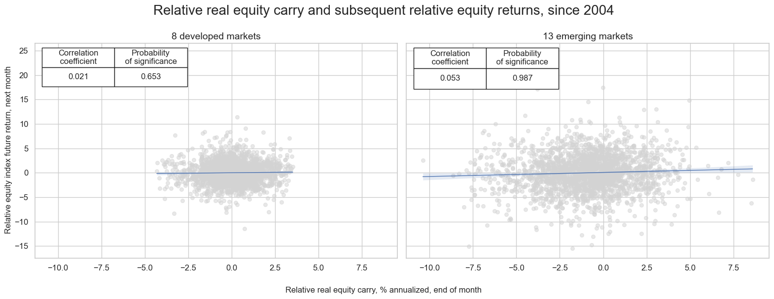
The predictive power of equity carry arises not solely from intertemporal relations (high carry today predicts high returns tomorrow) but also from cross-sectional relations (higher carry in country a versus country predicts higher return). This is show below by the relation between relative real index carry and relative subsequent equity returns for the developed and emerging markets country sets respectively. For both the predictive relation has been positive, albeit only for emerging countries the evidence has been statistically significant.

# Generate relative value data for DM and EM equities
xcatx = ["EQCRR_NSA", "EQXR_NSA", "EQCRR_VT10", "EQXR_VT10"]


dfa = msp.make_relative_value(
    dfx,
    xcats=xcatx,
    cids=cids_dmeq,
    rel_xcats=[xc + "vDM" for xc in xcatx],
)
dfx = msm.update_df(dfx, dfa)

dfa = msp.make_relative_value(
    dfx,
    xcats=xcatx,
    cids=cids_emeq,
    rel_xcats=[xc + "vEM" for xc in xcatx],
)

dfx = msm.update_df(dfx, dfa)

# Define common parameters
common_params = {
    "df": dfx,
    "freq": "m",
    "lag": 1,
    "xcat_aggs": ["last", "sum"],
    "blacklist": fxblack,
}

# Define CategoryRelations for Developed Markets
common_params["cids"] = cids_dmeq
cr_dm = msp.CategoryRelations(**common_params, xcats=["EQCRR_NSAvDM", "EQXR_NSAvDM"])

# Update parameters for Emerging Markets
common_params["cids"] = cids_emeq
cr_em = msp.CategoryRelations(**common_params, xcats=["EQCRR_NSAvEM", "EQXR_NSAvEM"])

# Define plot settings
msv.multiple_reg_scatter(
    [
        cr_dm,
        cr_em,
    ],
    title="Relative real equity carry and subsequent relative equity returns, since 2004",
    xlab="Relative real equity carry, % annualized, end of month",
    ylab="Relative equity index future return, next month",
    ncol=2,
    nrow=1,
    figsize=(16, 6),
    prob_est="map",
    subplot_titles=[
        f"{len(cids_dmeq)} developed markets",
        f"{len(cids_emeq)} emerging markets",
    ],
    coef_box="upper left",
)

Appendices

Appendix 1: Equity index specification

The following equity indices have been used for futures return calculations in each currency area:

• AUD: Standard and Poor’s / Australian Stock Exchange 200

• BRL: Brazil Bovespa

• CAD: Standard and Poor’s / Toronto Stock Exchange 60 Index

• CHF: Swiss Market (SMI)

• CNY: Shanghai Shenzhen CSI 300

• DEM: DAX 30 Performance (Xetra)

• ESP: IBEX 35

• EUR: EURO STOXX 50

• FRF: CAC 40

• GBP: FTSE 100

• HKD: Hang Seng China Enterprises

• INR: CNX Nifty (50)

• ITL: FTSE MIB Index

• JPY: Nikkei 225 Stock Average

• KRW: Korea Stock Exchange KOSPI 200

• MXN: Mexico IPC (Bolsa)

• MYR: FTSE Bursa Malaysia KLCI

• NLG: AEX Index (AEX)

• PLN: Warsaw General Index 20

• SEK: OMX Stockholm 30 (OMXS30)

• SGD: MSCI Singapore (Free)

• THB: Bangkok S.E.T. 50

• TRY: Bist National 30

• TWD: Taiwan Stock Exchange Weighed TAIEX

• USD: Standard and Poor’s 500 Composite

• ZAR: FTSE / JSE Top 40

For the older history of the Standard and Poor 500 (1990s), earnings yields have been used rather than the average of dividend and earnings yields.

See Appendix 3 for the list of currency symbols used to represent each cross-section.

Appendix 2: Alternative equity index specification

Alternative equity indices are available for the following currency areas:

• HKD: Hang Seng

• JPY: TOPIX

• USD: NASDAQ 100

• USD: Russell 2000

See Appendix 3 for the list of currency symbols used to represent each cross-section.

Appendix 3: Currency symbols

The word ‘cross-section’ refers to currencies, currency areas or economic areas. In alphabetical order, these are AUD (Australian dollar), BRL (Brazilian real), CAD (Canadian dollar), CHF (Swiss franc), CLP (Chilean peso), CNY (Chinese yuan renminbi), COP (Colombian peso), CZK (Czech Republic koruna), DEM (German mark), ESP (Spanish peseta), EUR (Euro), FRF (French franc), GBP (British pound), HKD (Hong Kong dollar), HUF (Hungarian forint), IDR (Indonesian rupiah), ITL (Italian lira), JPY (Japanese yen), KRW (Korean won), MXN (Mexican peso), MYR (Malaysian ringgit), NLG (Dutch guilder), NOK (Norwegian krone), NZD (New Zealand dollar), PEN (Peruvian sol), PHP (Phillipine peso), PLN (Polish zloty), RON (Romanian leu), RUB (Russian ruble), SEK (Swedish krona), SGD (Singaporean dollar), THB (Thai baht), TRY (Turkish lira), TWD (Taiwanese dollar), USD (U.S. dollar), ZAR (South African rand).