Diversified trend following in emerging FX markets

Get packages and JPMaQS data

# Set up environment

import numpy as np
import pandas as pd
import matplotlib.pyplot as plt
import seaborn as sns
from scipy.stats import norm
import itertools


import macrosynergy.management as msm
import macrosynergy.panel as msp
import macrosynergy.signal as mss
import macrosynergy.pnl as msn
import macrosynergy.visuals as msv
from macrosynergy.download import JPMaQSDownload
from macrosynergy.management.utils import merge_categories


from datetime import timedelta, date, datetime
from itertools import combinations
import warnings
import os

warnings.simplefilter("ignore")

# Cross section lists

cids_g3 = ["EUR", "JPY", "USD"]  # DM large currency areas
cids_dmsc = ["AUD", "CAD", "CHF", "GBP", "NOK", "NZD", "SEK"]  # DM small currency areas
cids_latm = ["BRL", "COP", "CLP", "MXN", "PEN"]  # Latam
cids_emea = ["CZK", "HUF", "ILS", "PLN", "RON", "RUB", "TRY", "ZAR"]  # EMEA
cids_emas = ["IDR", "INR", "KRW", "MYR", "PHP", "THB", "TWD"]  # EM Asia ex China

cids_dm = cids_g3 + cids_dmsc
cids_em = cids_latm + cids_emea + cids_emas
cids = cids_dm + cids_em
cids.sort()

# FX cross-section lists

cids_nofx = ["EUR", "USD", "RUB"]  # not suitable for analysis
cids_fx = list(set(cids) - set(cids_nofx))
cids_fx.sort()

cids_dmfx = list(set(cids_dm).intersection(cids_fx))
cids_dmfx.sort()
cids_emfx = list(set(cids_em).intersection(cids_fx))
cids_emfx.sort()

cids_eur = ["CHF", "CZK", "HUF", "NOK", "PLN", "RON", "SEK"]  # trading against EUR
cids_eud = ["GBP", "TRY"]  # trading against EUR and USD
cids_usd = list(set(cids_fx) - set(cids_eur + cids_eud))  # trading against USD

# Category lists

xbts = [  # long-term trends
    "MTBGDPRATIO_SA_3MMAv60MMA",
    "CABGDPRATIO_SA_3MMAv60MMA",
    "CABGDPRATIO_SA_1QMAv20QMA",
]

xbds = [  # shorter-term dynamcis
    "MTBGDPRATIO_SA_3MMA_D1M1ML3",
    "MTBGDPRATIO_SA_6MMA_D1M1ML6",
    "CABGDPRATIO_SA_3MMA_D1M1ML3",
    "CABGDPRATIO_SA_1QMA_D1Q1QL1"
]

xbs = xbts + xbds

niip = [  # NIIP
    "NIIPGDP_NSA_D1M1ML12",
    "NIIPGDP_NSA_D1Mv2YMA",
    "NIIPGDP_NSA_D1Mv5YMA",
]

il = [  # International Liabilities
    "IIPLIABGDP_NSA_D1M1ML12",
    "IIPLIABGDP_NSA_D1Mv2YMA",
    "IIPLIABGDP_NSA_D1Mv5YMA",
]

nils = niip + il

gdp = [
    # Intutive growth estimates
    "INTRGDP_NSA_P1M1ML12_3MMA",
    "INTRGDPv5Y_NSA_P1M1ML12_3MMA",
    "INTRGDP_NSA_P1M1ML12_D3M3ML3",
    # Technical growth estimates
    "RGDPTECH_SA_P1M1ML12_3MMA",
    "RGDPTECHv5Y_SA_P1M1ML12_3MMA",
    "RGDPTECH_SA_P1M1ML12_D3M3ML3",
]

# Excess inflation
cpi = [
    "CPIH_SA_P1M1ML12",
    "CPIH_SJA_P6M6ML6AR",
    "CPIC_SA_P1M1ML12",
    "CPIC_SJA_P6M6ML6AR",
]

cpi_aux = [
    "INFTEFF_NSA", 
    "INFTARGET_NSA",
    "INFE2Y_JA" 
]

inf = cpi + cpi_aux

reer = [ # Real appreciation
    "REER_NSA_P1M12ML1", 
    "REER_NSA_P1M60ML1"
    ]

pcr = [
    "PCREDITBN_SJA_P1M1ML12", 
    "PCREDITGDP_SJA_D1M1ML12"
    ]

exp = [
    "EXPORTS_SA_P1M1ML12_3MMA",
    "EXPORTS_SA_P6M6ML6AR",
]

oth = reer + pcr + exp

main = xbs + nils + gdp + inf + oth

rets = [
    "FXXR_NSA",
    "FXXR_VT10",
    "FXCRY_NSA",
    "EQXR_NSA",
    "FXTARGETED_NSA",
    "FXUNTRADABLE_NSA",
]

xcats = main + rets

# Resultant tickers

tickers = [cid + "_" + xcat for cid in cids for xcat in xcats]
print(f"Maximum number of tickers is {len(tickers)}")

Maximum number of tickers is 1140

# Download series from J.P. Morgan DataQuery by tickers

start_date = "1998-01-01"
end_date = None

# Retrieve credentials

client_id: str = os.getenv("DQ_CLIENT_ID")
client_secret: str = os.getenv("DQ_CLIENT_SECRET")

with JPMaQSDownload(client_id=client_id, client_secret=client_secret) as dq:
    df = dq.download(
        tickers=tickers,
        start_date=start_date,
        end_date=end_date,
        suppress_warning=True,
        metrics=["value"],
        report_time_taken=True,
        show_progress=True,
    )

Downloading data from JPMaQS.
Timestamp UTC:  2025-10-23 16:09:02
Connection successful!

Requesting data: 100%|██████████| 57/57 [00:11<00:00,  4.94it/s]
Downloading data: 100%|██████████| 57/57 [01:49<00:00,  1.93s/it] 

Time taken to download data: 	125.65 seconds.
Some expressions are missing from the downloaded data. Check logger output for complete list.
79 out of 1140 expressions are missing. To download the catalogue of all available expressions and filter the unavailable expressions, set `get_catalogue=True` in the call to `JPMaQSDownload.download()`.

dfx = df.copy()
dfx.info()

<class 'pandas.core.frame.DataFrame'>
RangeIndex: 7151073 entries, 0 to 7151072
Data columns (total 4 columns):
 #   Column     Dtype         
---  ------     -----         
 0   real_date  datetime64[ns]
 1   cid        object        
 2   xcat       object        
 3   value      float64       
dtypes: datetime64[ns](1), float64(1), object(2)
memory usage: 218.2+ MB

Blacklist, renamings, and availability check

Blacklist dictionary

dfb = df[df["xcat"].isin(["FXTARGETED_NSA", "FXUNTRADABLE_NSA"])].loc[
    :, ["cid", "xcat", "real_date", "value"]
]
dfba = (
    dfb.groupby(["cid", "real_date"])
    .aggregate(value=pd.NamedAgg(column="value", aggfunc="max"))
    .reset_index()
)
dfba["xcat"] = "FXBLACK"
fxblack = msp.make_blacklist(dfba, "FXBLACK")
fxblack

{'BRL': (Timestamp('2012-12-03 00:00:00'), Timestamp('2013-09-30 00:00:00')),
 'CHF': (Timestamp('2011-10-03 00:00:00'), Timestamp('2015-01-30 00:00:00')),
 'CZK': (Timestamp('2014-01-01 00:00:00'), Timestamp('2017-07-31 00:00:00')),
 'ILS': (Timestamp('1999-01-01 00:00:00'), Timestamp('2005-12-30 00:00:00')),
 'INR': (Timestamp('1999-01-01 00:00:00'), Timestamp('2004-12-31 00:00:00')),
 'MYR_1': (Timestamp('1999-01-01 00:00:00'), Timestamp('2007-11-30 00:00:00')),
 'MYR_2': (Timestamp('2018-07-02 00:00:00'), Timestamp('2025-10-22 00:00:00')),
 'PEN': (Timestamp('2021-07-01 00:00:00'), Timestamp('2021-07-30 00:00:00')),
 'RON': (Timestamp('1999-01-01 00:00:00'), Timestamp('2005-11-30 00:00:00')),
 'RUB_1': (Timestamp('1999-01-01 00:00:00'), Timestamp('2005-11-30 00:00:00')),
 'RUB_2': (Timestamp('2022-02-01 00:00:00'), Timestamp('2025-10-22 00:00:00')),
 'THB': (Timestamp('2007-01-01 00:00:00'), Timestamp('2008-11-28 00:00:00')),
 'TRY_1': (Timestamp('1999-01-01 00:00:00'), Timestamp('2003-09-30 00:00:00')),
 'TRY_2': (Timestamp('2020-01-01 00:00:00'), Timestamp('2024-07-31 00:00:00'))}

Availability check

# Replace quarterly tickers with approximately equivalent monthly tickers

dict_repl = {
    "CABGDPRATIO_SA_1QMAv20QMA": "CABGDPRATIO_SA_3MMAv60MMA",
    "CABGDPRATIO_SA_1QMA_D1Q1QL1": "CABGDPRATIO_SA_3MMA_D1M1ML3",
}
dfx["xcat"] = dfx["xcat"].replace(dict_repl, regex=False)

xcatx = [xb for xb in xbs if xb not in dict_repl.keys()]
cidx = cids
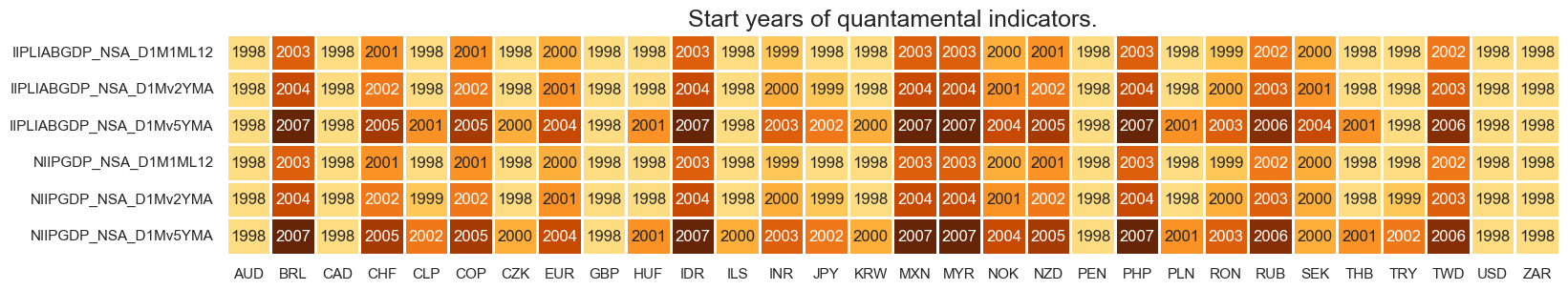
msm.check_availability(dfx, xcats=xcatx, cids=cidx, missing_recent=False)

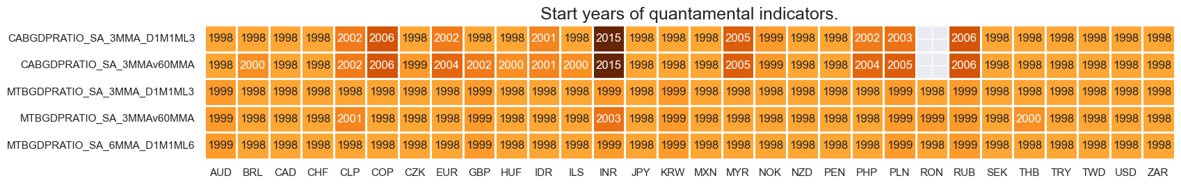
xcatx = nils
cidx = cids
msm.check_availability(dfx, xcats=xcatx, cids=cidx, missing_recent=False)

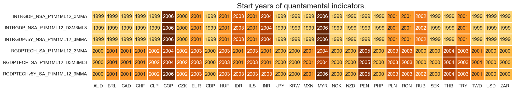
xcatx = gdp
cidx = cids
msm.check_availability(dfx, xcats=xcatx, cids=cidx, missing_recent=False)

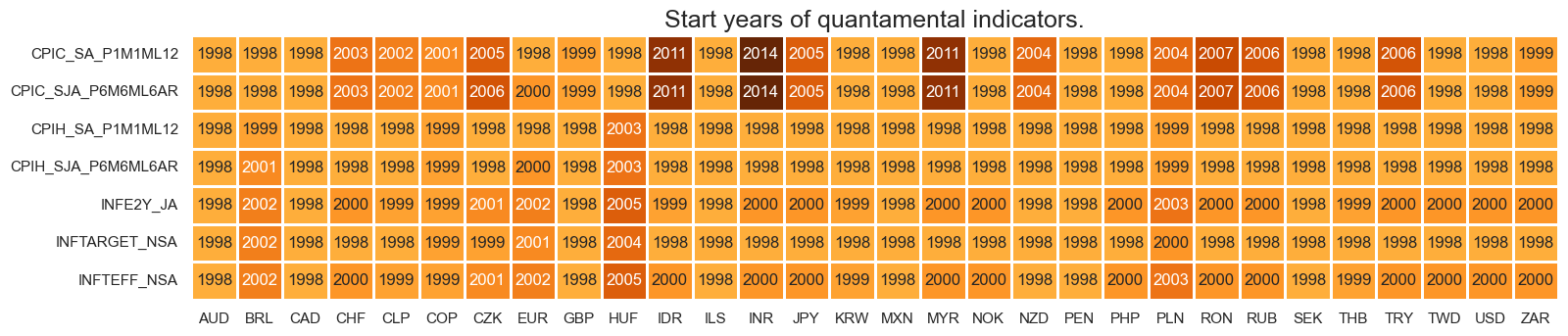
xcatx = inf
cidx = cids
msm.check_availability(dfx, xcats=xcatx, cids=cidx, missing_recent=False)

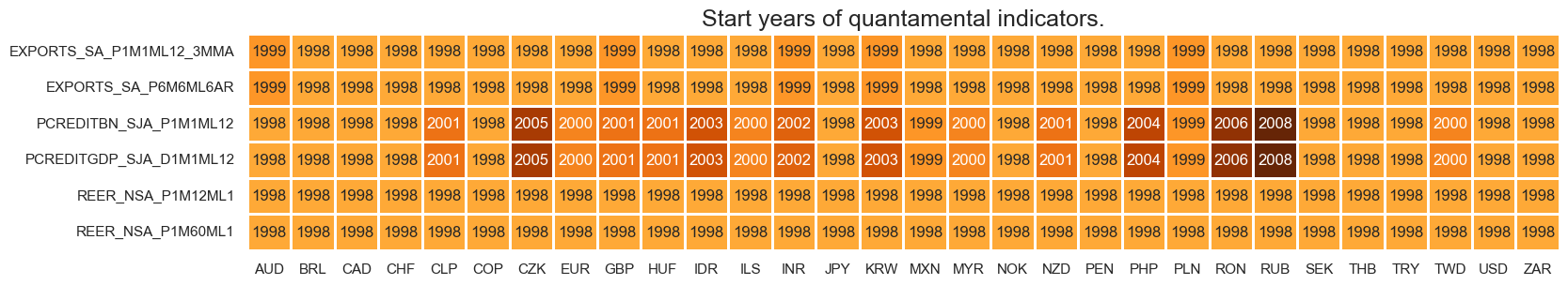
xcatx = oth
cidx = cids
msm.check_availability(dfx, xcats=xcatx, cids=cidx, missing_recent=False)

Feature engineering and checks

External balance trends

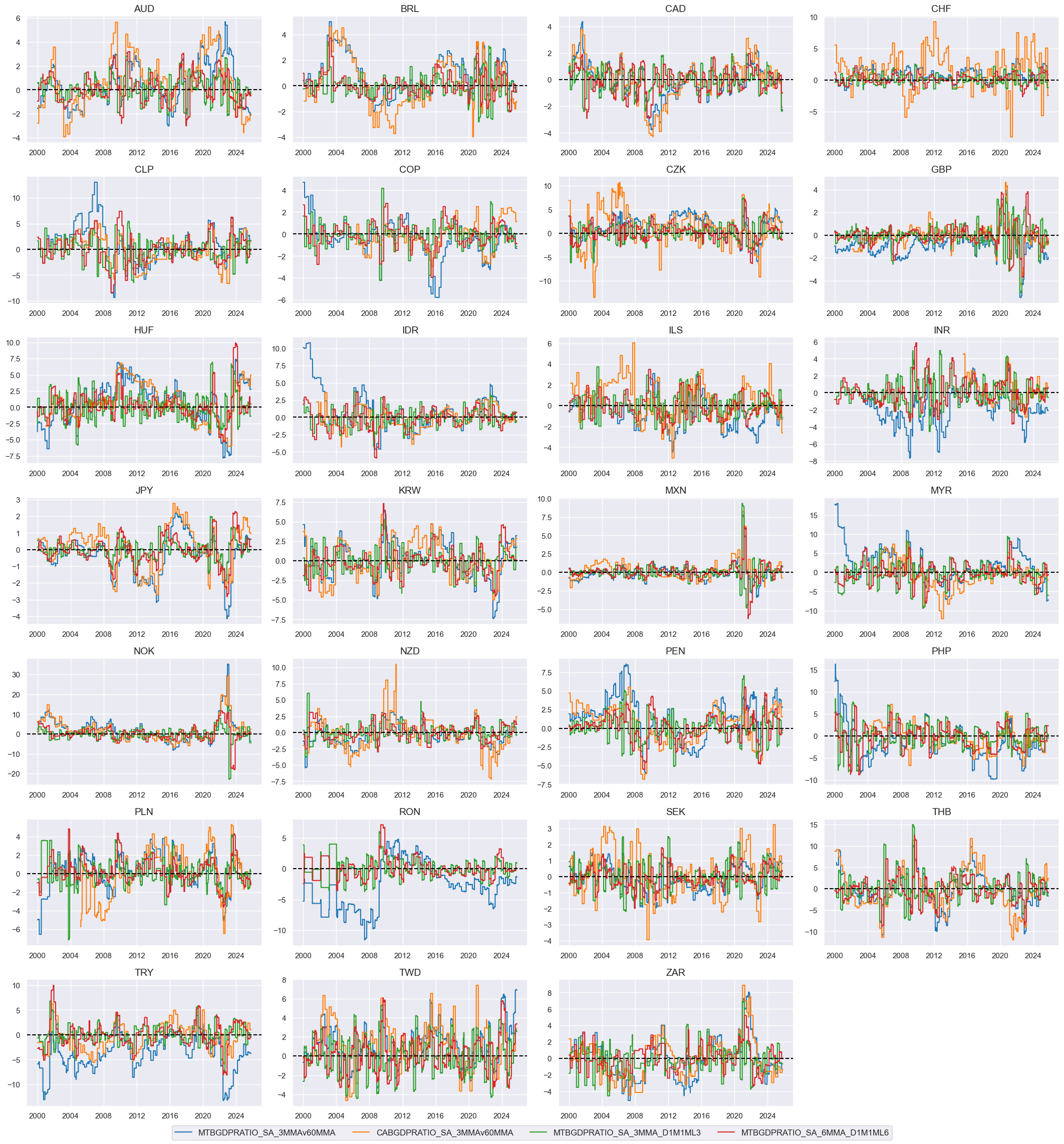
# Indicator list and visualization

xbx = [
    "MTBGDPRATIO_SA_3MMAv60MMA",
    "CABGDPRATIO_SA_3MMAv60MMA",
    "MTBGDPRATIO_SA_3MMA_D1M1ML3",
    "MTBGDPRATIO_SA_6MMA_D1M1ML6",
]

xcatx = xbx
cidx = cids_fx

msp.view_timelines(
    dfx,
    xcats=xcatx,
    cids=cidx,
    ncol=4,
    start="2000-01-01",
    same_y=False,
    height=2.2,
    size=(10, 10),
    all_xticks=True,
)

# Indicator scores

xcatx = xbx  # shorter term dynamics
cidx = cids_fx

dfa = pd.DataFrame(columns=dfx.columns)
for xc in xcatx:
    dfaa = msp.make_zn_scores(
        dfx,
        xcat=xc,
        cids=cidx,
        sequential=True,
        min_obs=522,  # oos scaling after 2 years of panel data
        est_freq="m",
        neutral="zero",
        pan_weight=1,
        thresh=3,
        postfix="_ZN",
    )
    dfa = msm.update_df(dfa, dfaa)
dfx = msm.update_df(dfx, dfa)

# Weighted factor score

dict_indx = {
    "MTBGDPRATIO_SA_3MMA_D1M1ML3_ZN": 1 / 4,
    "MTBGDPRATIO_SA_6MMA_D1M1ML6_ZN": 1 / 4,
    "MTBGDPRATIO_SA_3MMAv60MMA_ZN": 1 / 4,
    "CABGDPRATIO_SA_3MMAv60MMA_ZN": 1 / 4,
}
fact = "XBTREND"

xcatx = list(dict_indx.keys())
weights = list(dict_indx.values())
cidx = cids_fx

# Create weighted composite

dfa = msp.linear_composite(
    dfx,
    xcats=xcatx,
    weights=weights,
    cids=cidx,
    complete_xcats=False,
    new_xcat=fact,
)
dfx = msm.update_df(dfx, dfa)

# Re-score the composite factor

dfa = msp.make_zn_scores(
    dfx,
    xcat=fact,
    cids=cidx,
    sequential=True,
    min_obs=522,  # oos scaling after 2 years of panel data
    est_freq="m",
    neutral="zero",
    pan_weight=1,
    thresh=3,
    postfix="_ZN",
)

dfx = msm.update_df(dfx, dfa)

# Visualize factor score

msp.view_timelines(
    dfx,
    xcats=[fact + "_ZN"],
    cids=cidx,
    ncol=4,
    start="2000-01-01",
    same_y=True,
    height=2.2,
    size=(10, 10),
    all_xticks=True,
)

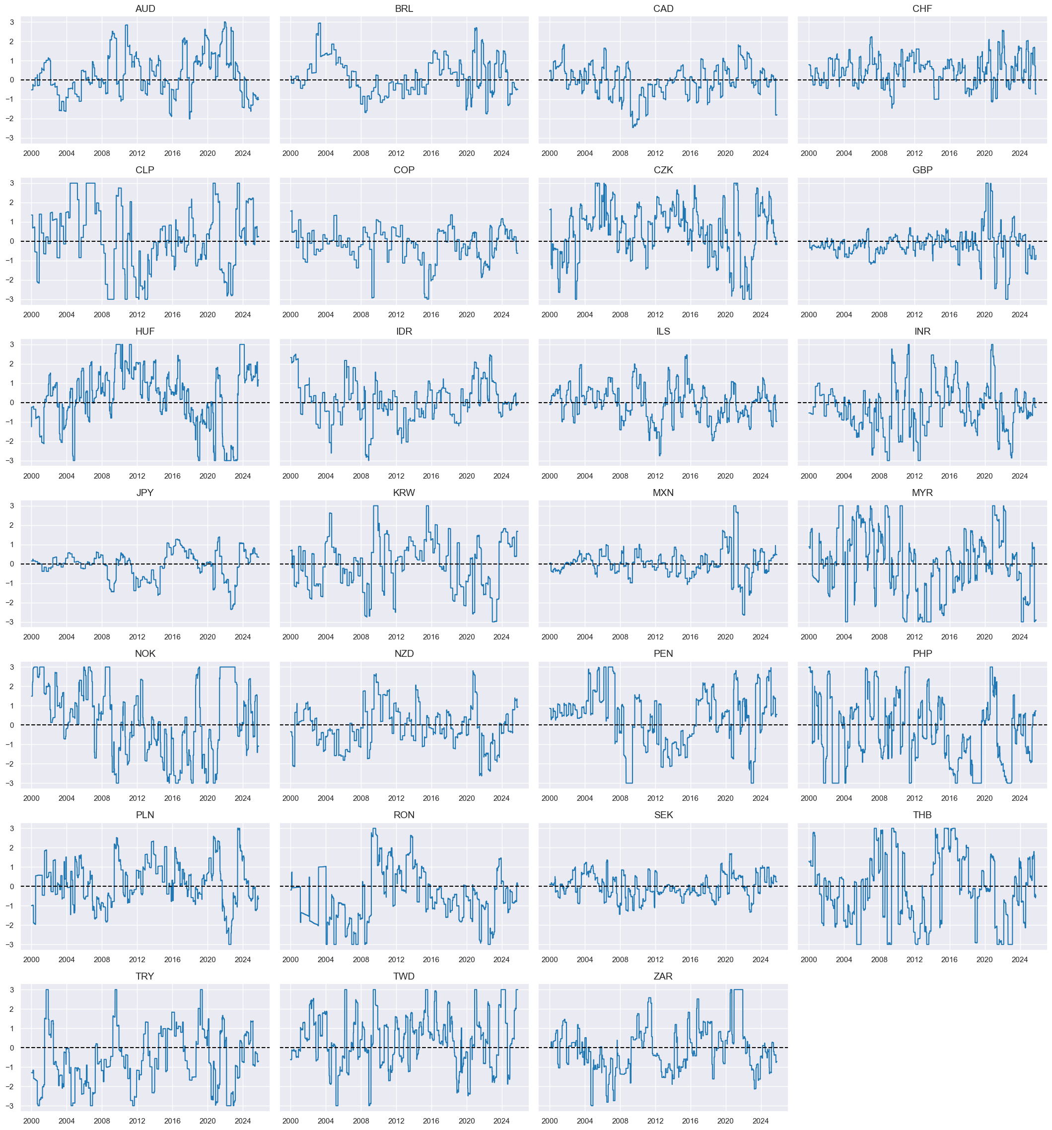
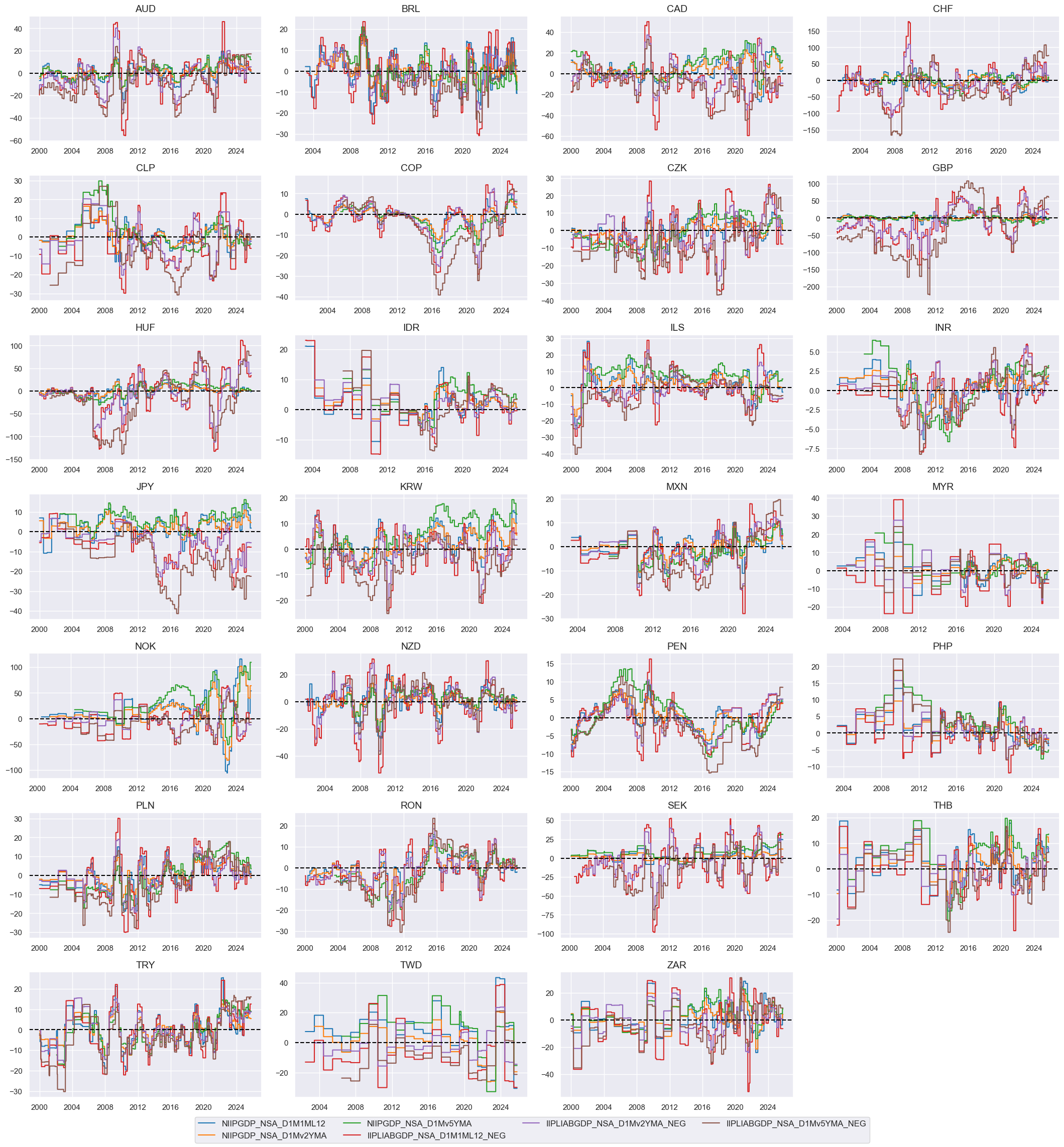
International investment trends

# Change sign of liability growth

xcatx = nils
cidx = cids_fx

calcs = []

for xc in xcatx:
    if "IIPLIABGDP" in xc:
        calcs.append(f"{xc}_NEG = - {xc}")
dfa = msp.panel_calculator(dfx, calcs=calcs, cids=cidx)
dfx = msm.update_df(dfx, dfa)

# Indicator list and visualization

nilx = [
    "NIIPGDP_NSA_D1M1ML12",
    "NIIPGDP_NSA_D1Mv2YMA",
    "NIIPGDP_NSA_D1Mv5YMA",
    "IIPLIABGDP_NSA_D1M1ML12_NEG",
    "IIPLIABGDP_NSA_D1Mv2YMA_NEG",
    "IIPLIABGDP_NSA_D1Mv5YMA_NEG",
]

xcatx = nilx
cidx = cids_fx

msp.view_timelines(
    dfx,
    xcats=xcatx,
    cids=cidx,
    ncol=4,
    start="2000-01-01",
    same_y=False,
    height=2.2,
    size=(10, 10),
    all_xticks=True,
)

# Indicator scores

xcatx = nilx  # shorter term dynamics
cidx = cids_fx

dfa = pd.DataFrame(columns=dfx.columns)
for xc in xcatx:
    dfaa = msp.make_zn_scores(
        dfx,
        xcat=xc,
        cids=cidx,
        sequential=True,
        min_obs=522,  # oos scaling after 2 years of panel data
        est_freq="m",
        neutral="zero",
        pan_weight=1,
        thresh=3,
        postfix="_ZN",
    )
    dfa = msm.update_df(dfa, dfaa)
dfx = msm.update_df(dfx, dfa)

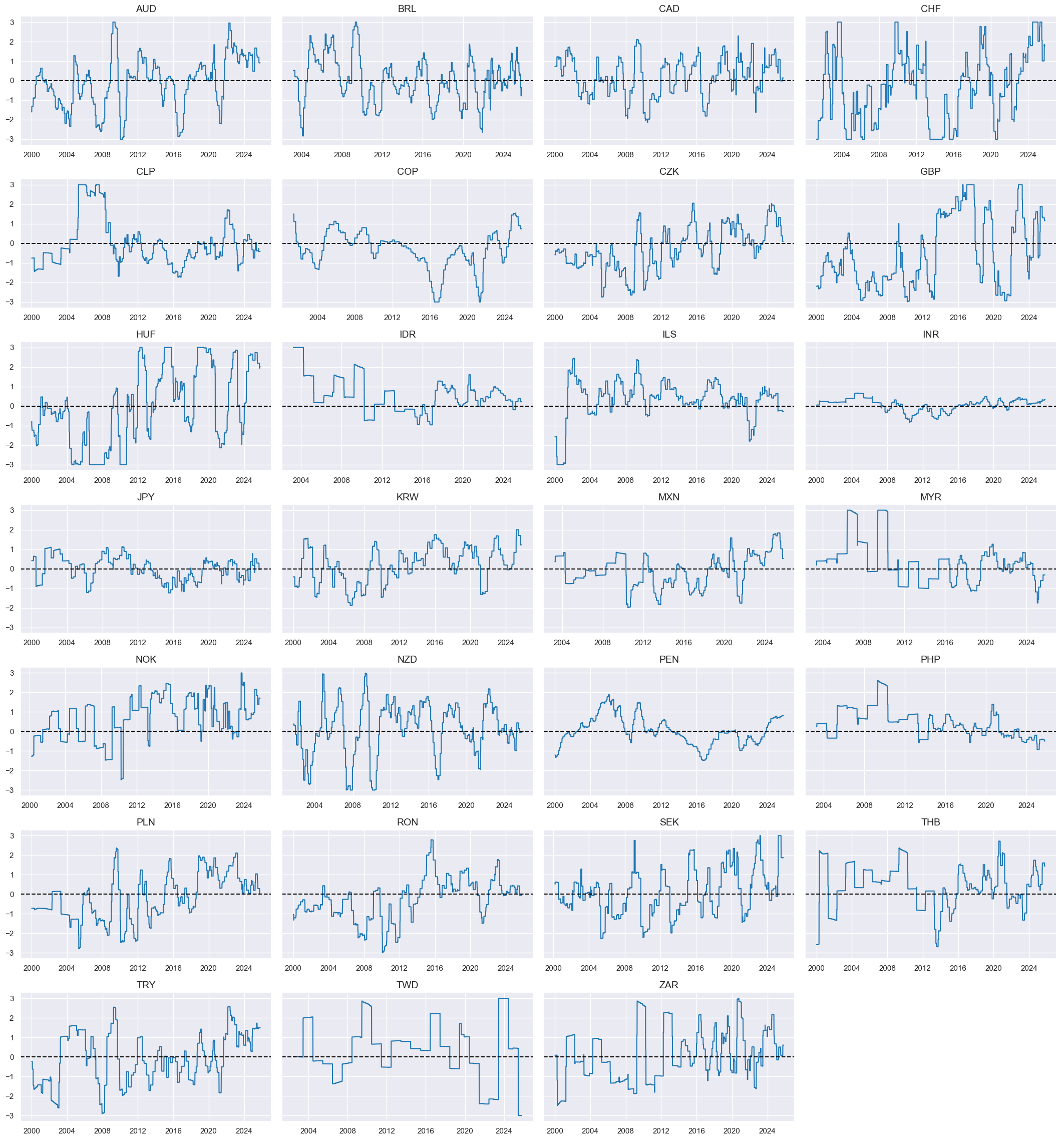
# Weighted factor score

dict_indx = {
    "NIIPGDP_NSA_D1M1ML12_ZN": 1 / 6,
    "NIIPGDP_NSA_D1Mv2YMA_ZN": 1 / 6,
    "NIIPGDP_NSA_D1Mv5YMA_ZN": 1 / 6,
    "IIPLIABGDP_NSA_D1M1ML12_NEG_ZN": 1 / 6,
    "IIPLIABGDP_NSA_D1Mv2YMA_NEG_ZN": 1 / 6,
    "IIPLIABGDP_NSA_D1Mv5YMA_NEG_ZN": 1 / 6,
}
fact = "IITREND"

xcatx = list(dict_indx.keys())
weights = list(dict_indx.values())
cidx = cids_fx

# Create weighted composite

dfa = msp.linear_composite(
    dfx,
    xcats=xcatx,
    weights=weights,
    cids=cidx,
    complete_xcats=False,
    new_xcat=fact,
)
dfx = msm.update_df(dfx, dfa)

# Re-score the composite factor

dfa = msp.make_zn_scores(
    dfx,
    xcat=fact,
    cids=cidx,
    sequential=True,
    min_obs=522,  # oos scaling after 2 years of panel data
    est_freq="m",
    neutral="zero",
    pan_weight=1,
    thresh=3,
    postfix="_ZN",
)

dfx = msm.update_df(dfx, dfa)

# Visualize factor score

msp.view_timelines(
    dfx,
    xcats=[fact + "_ZN"],
    cids=cidx,
    ncol=4,
    start="2000-01-01",
    same_y=True,
    height=2.2,
    size=(10, 10),
    all_xticks=True,
)

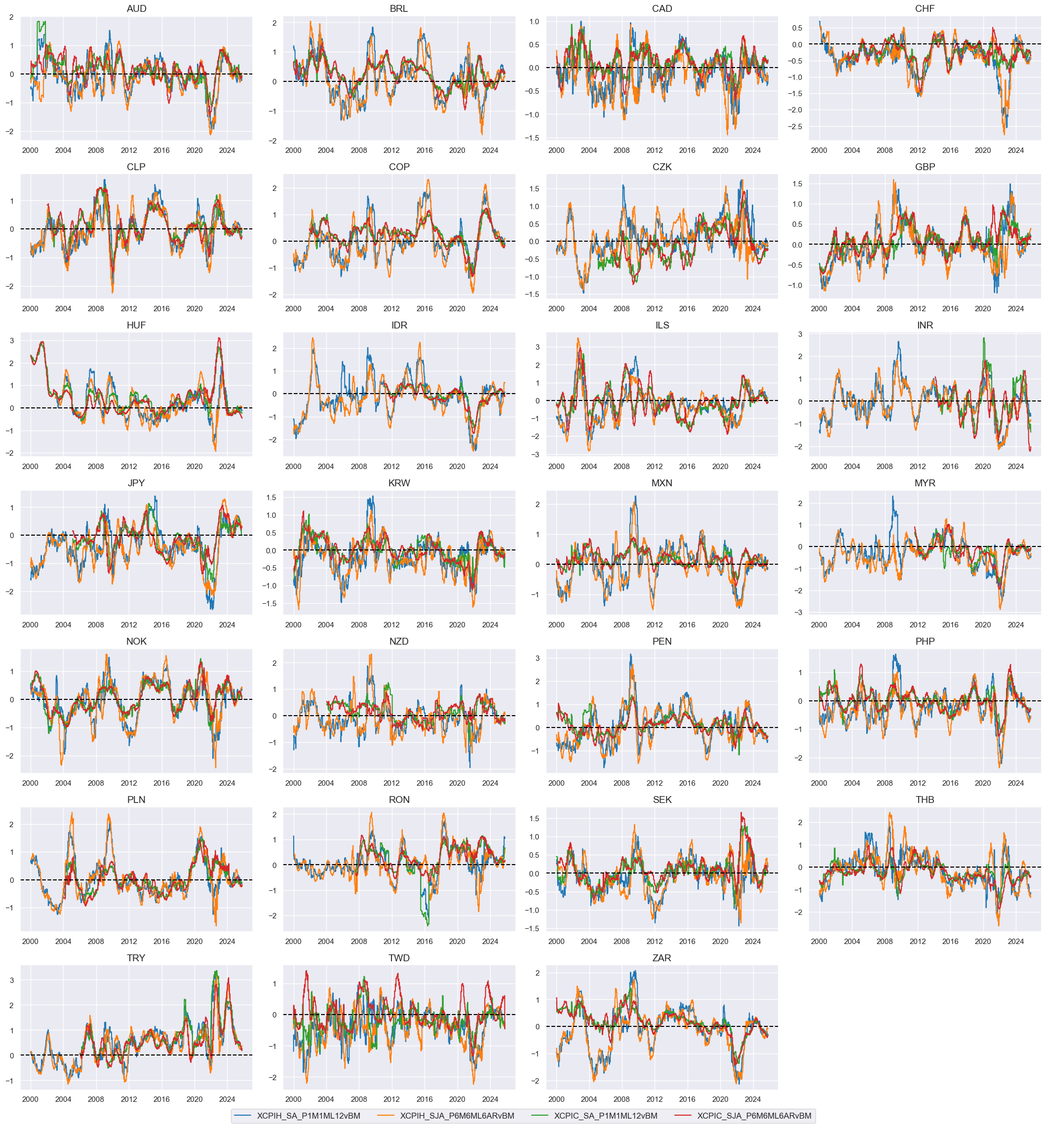
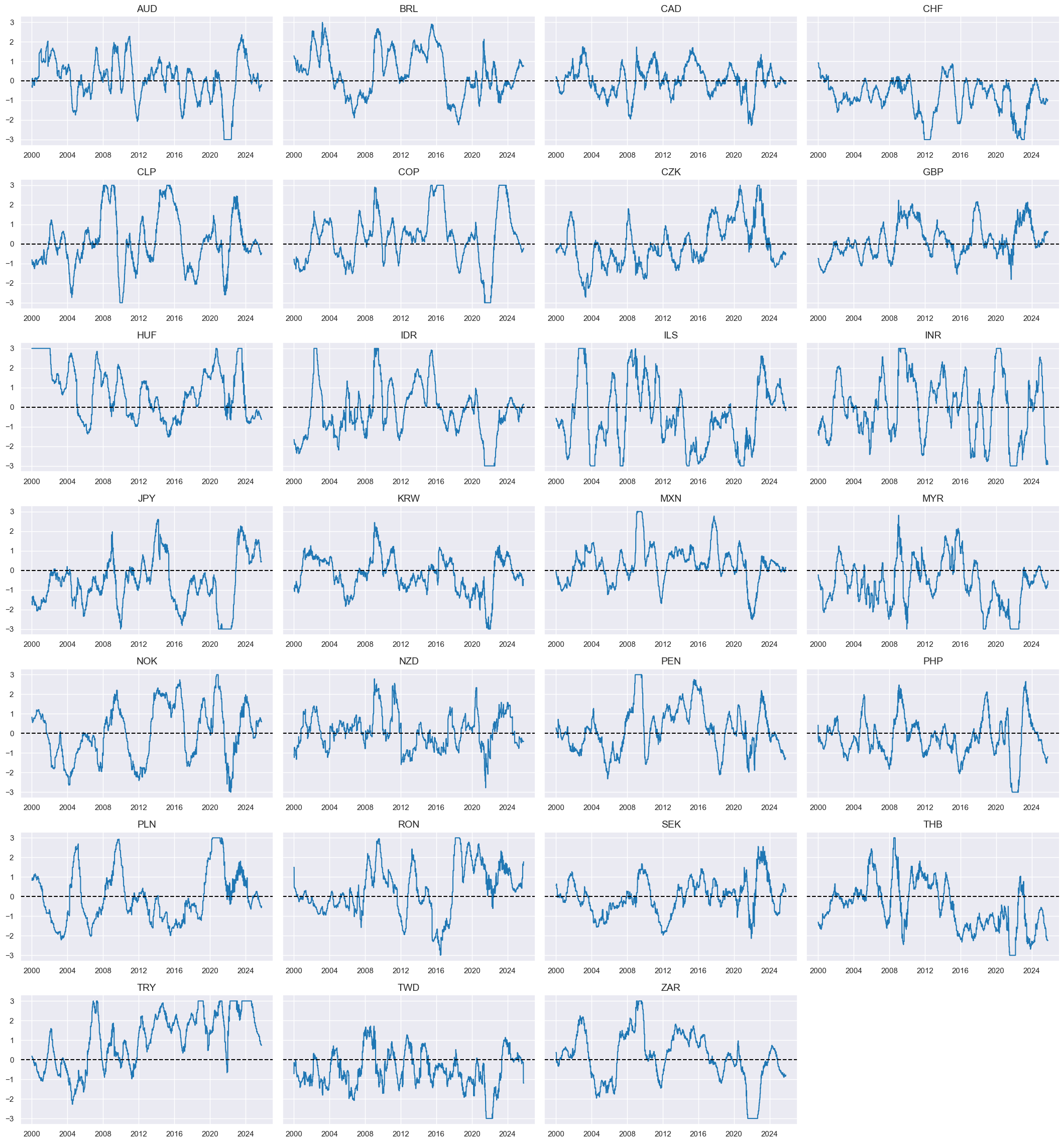
Relative excess inflation rates

# Backward-extension of INFTARGET_NSA

# Duplicate targets
cidx = cids
calcs = [f"INFTARGET_BX = INFTARGET_NSA"]
dfa = msp.panel_calculator(dfx, calcs, cids=cidx)

# Add all dates back to 1990 to the frame, filling "value " with NaN
all_dates = np.sort(dfx['real_date'].unique())
all_combinations = pd.DataFrame(
    list(itertools.product(dfa['cid'].unique(), dfa['xcat'].unique(), all_dates)),
    columns=['cid', 'xcat', 'real_date']
)
dfax = pd.merge(all_combinations, dfa, on=['cid', 'xcat', 'real_date'], how='left')

# Backfill the values with first target value
dfax = dfax.sort_values(by=['cid', 'xcat', 'real_date'])
dfax['value'] = dfax.groupby(['cid', 'xcat'])['value'].bfill()

dfx = msm.update_df(dfx, dfax)

# Extended effective inflation target by hierarchical merging

hierarchy = ["INFTEFF_NSA", "INFTARGET_BX"]
dfa = merge_categories(dfx, xcats=hierarchy, new_xcat="INFTEFF_BX")
dfx = msm.update_df(dfx, dfa)

# Excess inflation rates relative to target inflation - minimum denominator of 2% to avoid extreme values

xcatx = cpi
calcs = [f"X{xc} = ( {xc} - INFTEFF_BX ) / np.clip( INFTEFF_BX , 2 , 9999 )" for xc in xcatx]

dfa = msp.panel_calculator(
    dfx,
    calcs=calcs,
    cids=cids,
)
dfx = msm.update_df(dfx, dfa)

# Relative excess inflation rates

xcatx = cpi

dfa = pd.DataFrame(columns=list(dfx.columns))
for xc in xcatx:
    calc_eur = [f"X{xc}vBM = X{xc} - iEUR_X{xc}"]
    calc_usd = [f"X{xc}vBM = X{xc} - iUSD_X{xc}"]
    calc_eud = [f"X{xc}vBM = X{xc} - 0.5 * ( iEUR_X{xc} + iUSD_X{xc} )"]

    dfa_eur = msp.panel_calculator(dfx, calcs=calc_eur, cids=cids_eur)
    dfa_usd = msp.panel_calculator(dfx, calcs=calc_usd, cids=cids_usd)
    dfa_eud = msp.panel_calculator(dfx, calcs=calc_eud, cids=cids_eud)

    dfa = msm.update_df(dfa, pd.concat([dfa_eur, dfa_usd, dfa_eud]))

dfx = msm.update_df(dfx, dfa)

# Indicator list and visualization

rxi = [
    "XCPIH_SA_P1M1ML12vBM",
    "XCPIH_SJA_P6M6ML6ARvBM",
    "XCPIC_SA_P1M1ML12vBM",
    "XCPIC_SJA_P6M6ML6ARvBM",
]

xcatx = rxi
cidx = cids_fx

msp.view_timelines(
    dfx,
    xcats=xcatx,
    cids=cidx,
    ncol=4,
    start="2000-01-01",
    same_y=False,
    height=2.2,
    size=(10, 10),
    all_xticks=True,
)

# Indicator scores

xcatx = rxi
cidx = cids_fx

dfa = pd.DataFrame(columns=dfx.columns)
for xc in xcatx:
    dfaa = msp.make_zn_scores(
        dfx,
        xcat=xc,
        cids=cidx,
        sequential=True,
        min_obs=522,  # oos scaling after 2 years of panel data
        est_freq="m",
        neutral="zero",
        pan_weight=1,
        thresh=3,
        postfix="_ZN",
    )
    dfa = msm.update_df(dfa, dfaa)
dfx = msm.update_df(dfx, dfa)

# Weighted factor score

dict_indx = {
    "XCPIH_SA_P1M1ML12vBM_ZN": 1 / 4,
    "XCPIH_SJA_P6M6ML6ARvBM_ZN": 1 / 4,
    "XCPIC_SA_P1M1ML12vBM_ZN": 1 / 4,
    "XCPIC_SJA_P6M6ML6ARvBM_ZN": 1 / 4,
}
fact = "RXINFTREND"

xcatx = list(dict_indx.keys())
weights = list(dict_indx.values())
cidx = cids_fx

# Create weighted composite

dfa = msp.linear_composite(
    dfx,
    xcats=xcatx,
    weights=weights,
    cids=cidx,
    complete_xcats=False,
    new_xcat=fact,
)
dfx = msm.update_df(dfx, dfa)

# Re-score the composite factor

dfa = msp.make_zn_scores(
    dfx,
    xcat=fact,
    cids=cidx,
    sequential=True,
    min_obs=522,  # oos scaling after 2 years of panel data
    est_freq="m",
    neutral="zero",
    pan_weight=1,
    thresh=3,
    postfix="_ZN",
)

dfx = msm.update_df(dfx, dfa)

# Visualize factor score

msp.view_timelines(
    dfx,
    xcats=[fact + "_ZN"],
    cids=cidx,
    ncol=4,
    start="2000-01-01",
    same_y=True,
    height=2.2,
    size=(10, 10),
    all_xticks=True,
)

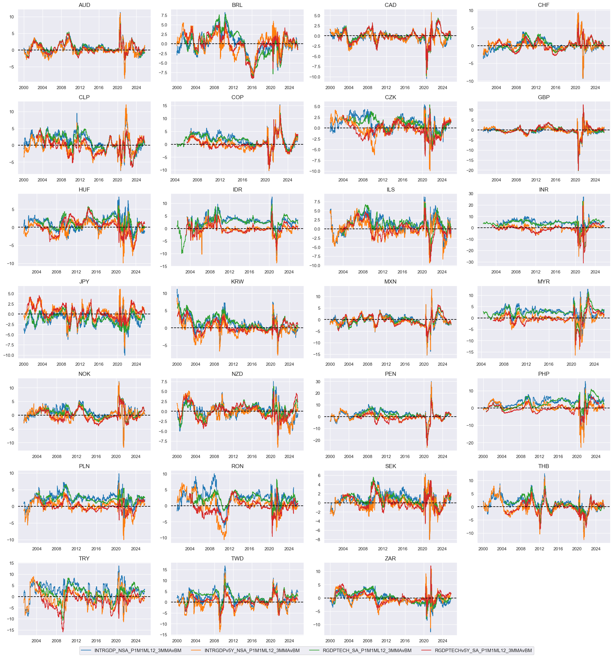
Relative growth trends

# Relative growth rates

grow = [
    "INTRGDP_NSA_P1M1ML12_3MMA",
    "INTRGDPv5Y_NSA_P1M1ML12_3MMA",
    "RGDPTECH_SA_P1M1ML12_3MMA",
    "RGDPTECHv5Y_SA_P1M1ML12_3MMA",
]
xcatx = grow

dfa = pd.DataFrame(columns=list(dfx.columns))
for xc in xcatx:
    calc_eur = [f"{xc}vBM = {xc} - iEUR_{xc}"]
    calc_usd = [f"{xc}vBM = {xc} - iUSD_{xc}"]
    calc_eud = [f"{xc}vBM = {xc} - 0.5 * ( iEUR_{xc} + iUSD_{xc} )"]

    dfa_eur = msp.panel_calculator(dfx, calcs=calc_eur, cids=cids_eur)
    dfa_usd = msp.panel_calculator(dfx, calcs=calc_usd, cids=cids_usd)
    dfa_eud = msp.panel_calculator(dfx, calcs=calc_eud, cids=cids_eud)

    dfa = msm.update_df(dfa, pd.concat([dfa_eur, dfa_usd, dfa_eud]))

dfx = msm.update_df(dfx, dfa)

# Indicator list and visualization

rgrow = [g + "vBM" for g in grow]

xcatx = rgrow
cidx = cids_fx

msp.view_timelines(
    dfx,
    xcats=xcatx,
    cids=cidx,
    ncol=4,
    start="2000-01-01",
    same_y=False,
    height=2.2,
    size=(10, 10),
    all_xticks=True,
)

# Indicator scores

xcatx = rgrow 
cidx = cids_fx

dfa = pd.DataFrame(columns=dfx.columns)
for xc in xcatx:
    dfaa = msp.make_zn_scores(
        dfx,
        xcat=xc,
        cids=cidx,
        sequential=True,
        min_obs=522,  # oos scaling after 2 years of panel data
        est_freq="m",
        neutral="zero",
        pan_weight=1,
        thresh=3,
        postfix="_ZN",
    )
    dfa = msm.update_df(dfa, dfaa)
dfx = msm.update_df(dfx, dfa)

# Weighted factor score

dict_indx = {
    "INTRGDP_NSA_P1M1ML12_3MMAvBM_ZN": 1 / 4,
    "INTRGDPv5Y_NSA_P1M1ML12_3MMAvBM_ZN": 1 / 4,
    "RGDPTECH_SA_P1M1ML12_3MMAvBM_ZN": 1 / 4,
    "RGDPTECHv5Y_SA_P1M1ML12_3MMAvBM_ZN": 1 / 4,
}
fact = "RGDPTREND"

xcatx = list(dict_indx.keys())
weights = list(dict_indx.values())
cidx = cids_fx

# Create weighted composite

dfa = msp.linear_composite(
    dfx,
    xcats=xcatx,
    weights=weights,
    cids=cidx,
    complete_xcats=False,
    new_xcat=fact,
)
dfx = msm.update_df(dfx, dfa)

# Re-score the composite factor

dfa = msp.make_zn_scores(
    dfx,
    xcat=fact,
    cids=cidx,
    sequential=True,
    min_obs=522,  # oos scaling after 2 years of panel data
    est_freq="m",
    neutral="zero",
    pan_weight=1,
    thresh=3,
    postfix="_ZN",
)

dfx = msm.update_df(dfx, dfa)

# Visualize factor score

msp.view_timelines(
    dfx,
    xcats=[fact + "_ZN"],
    cids=cidx,
    ncol=4,
    start="2000-01-01",
    same_y=True,
    height=2.2,
    size=(10, 10),
    all_xticks=True,
)

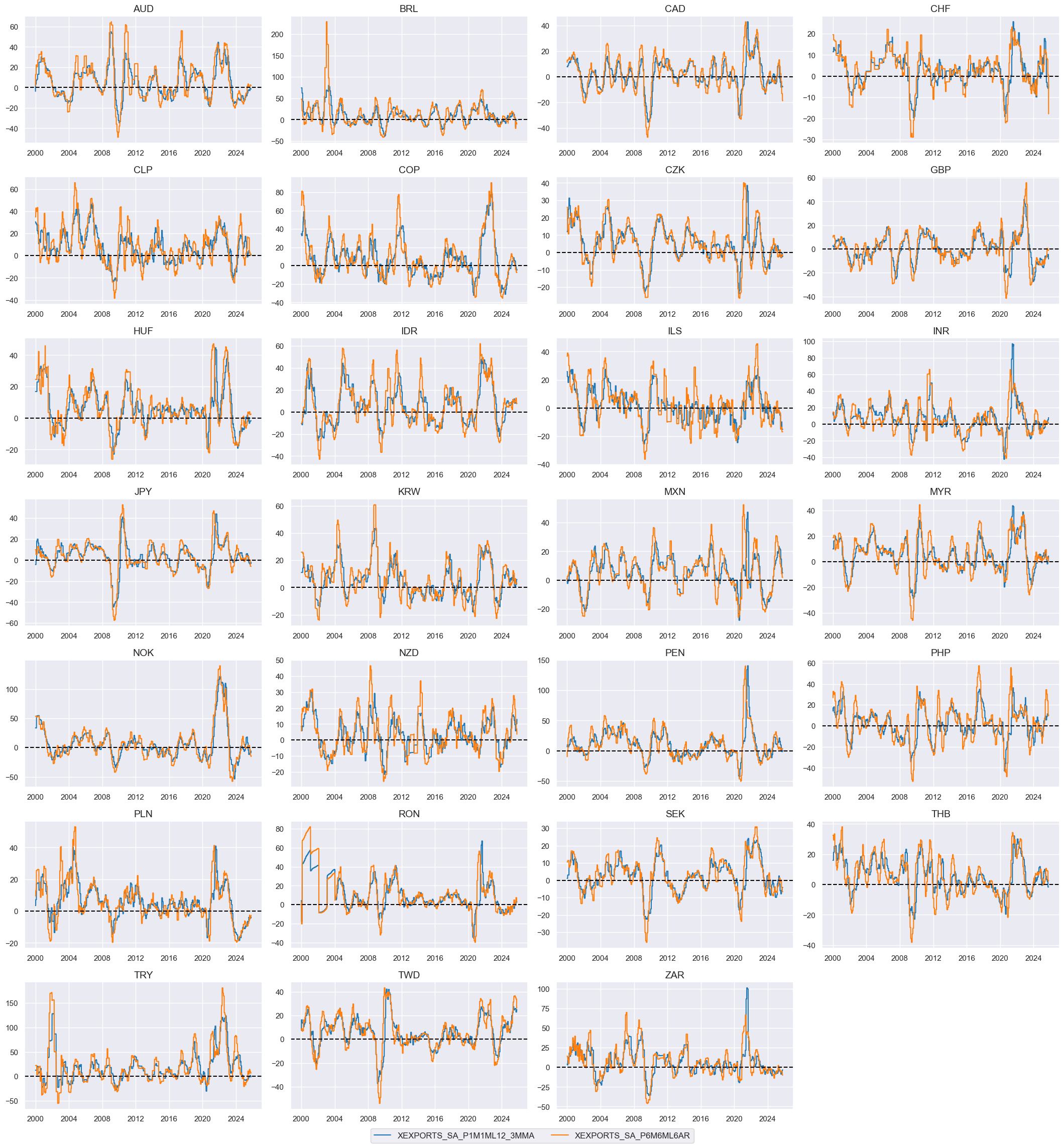
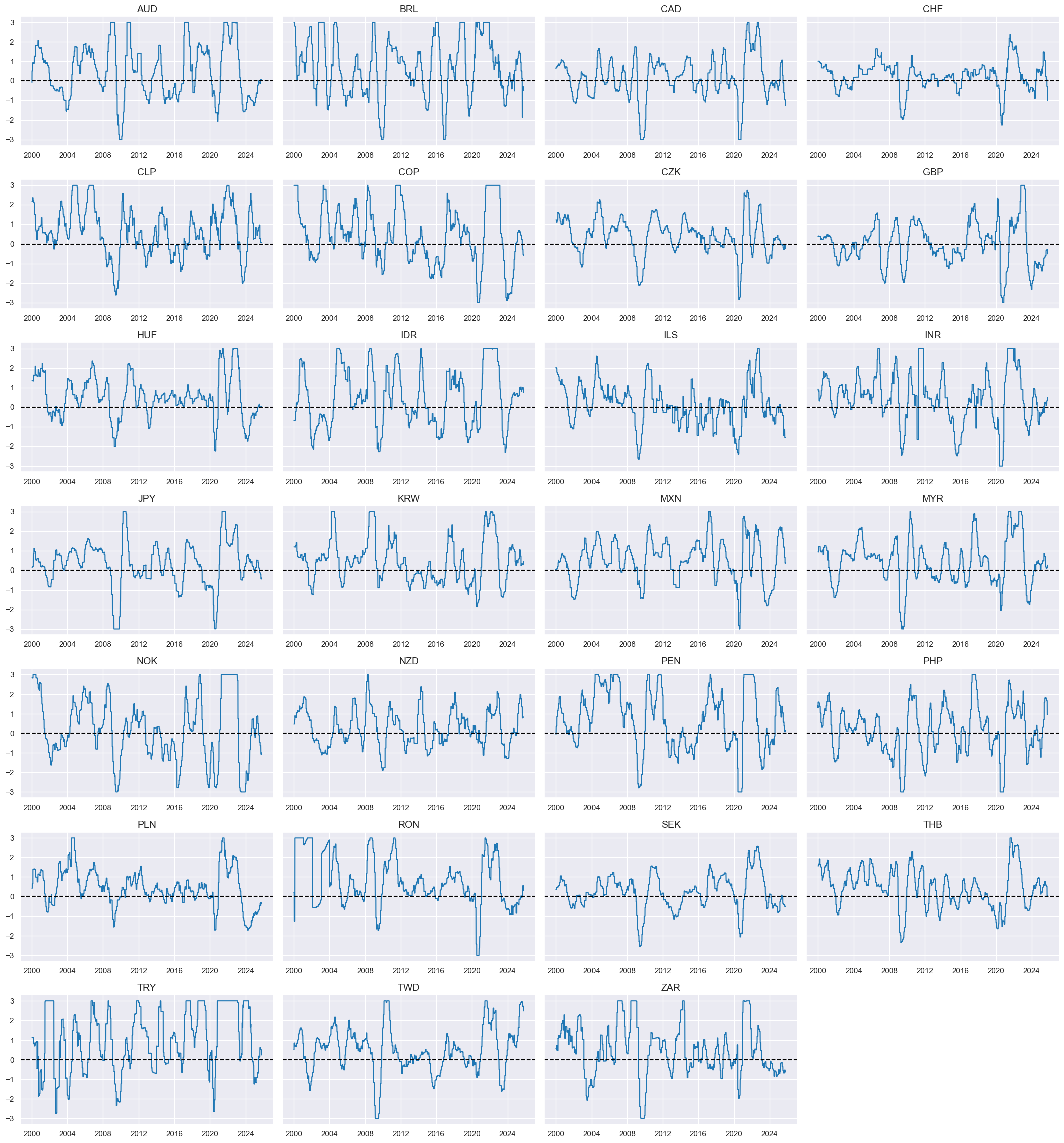
Local-currency currency export growth

# Excess export growth rates (in excess of inflation target)

lcexp = [
    "EXPORTS_SA_P1M1ML12_3MMA",
    "EXPORTS_SA_P6M6ML6AR",
]

xcatx = lcexp
calcs = [f"X{xc} = {xc} - ( INFTEFF_BX )" for xc in xcatx]

dfa = msp.panel_calculator(
    dfx,
    calcs=calcs,
    cids=cids,
)
dfx = msm.update_df(dfx, dfa)

xexp = ["X" + xc for xc in lcexp]
xcatx = xexp
cidx = cids_fx

msp.view_timelines(
    dfx,
    xcats=xcatx,
    cids=cidx,
    ncol=4,
    start="2000-01-01",
    same_y=False,
    height=2.2,
    size=(10, 10),
    all_xticks=True,
)

# Indicator scores

xcatx = xexp
cidx = cids_fx

dfa = pd.DataFrame(columns=dfx.columns)
for xc in xcatx:
    dfaa = msp.make_zn_scores(
        dfx,
        xcat=xc,
        cids=cidx,
        sequential=True,
        min_obs=522,  # oos scaling after 2 years of panel data
        est_freq="m",
        neutral="zero",
        pan_weight=1,
        thresh=3,
        postfix="_ZN",
    )
    dfa = msm.update_df(dfa, dfaa)
dfx = msm.update_df(dfx, dfa)

# Weighted factor score

dict_indx = {
    "XEXPORTS_SA_P1M1ML12_3MMA_ZN": 1 / 2,
    "XEXPORTS_SA_P6M6ML6AR_ZN": 1 / 2,
}
fact = "XEXPTREND"

xcatx = list(dict_indx.keys())
weights = list(dict_indx.values())
cidx = cids_fx

# Create weighted composite

dfa = msp.linear_composite(
    dfx,
    xcats=xcatx,
    weights=weights,
    cids=cidx,
    complete_xcats=False,
    new_xcat=fact,
)
dfx = msm.update_df(dfx, dfa)

# Re-score the composite factor

dfa = msp.make_zn_scores(
    dfx,
    xcat=fact,
    cids=cidx,
    sequential=True,
    min_obs=522,  # oos scaling after 2 years of panel data
    est_freq="m",
    neutral="zero",
    pan_weight=1,
    thresh=3,
    postfix="_ZN",
)

dfx = msm.update_df(dfx, dfa)

# Visualize factor score

msp.view_timelines(
    dfx,
    xcats=[fact + "_ZN"],
    cids=cidx,
    ncol=4,
    start="2000-01-01",
    same_y=True,
    height=2.2,
    size=(10, 10),
    all_xticks=True,
)

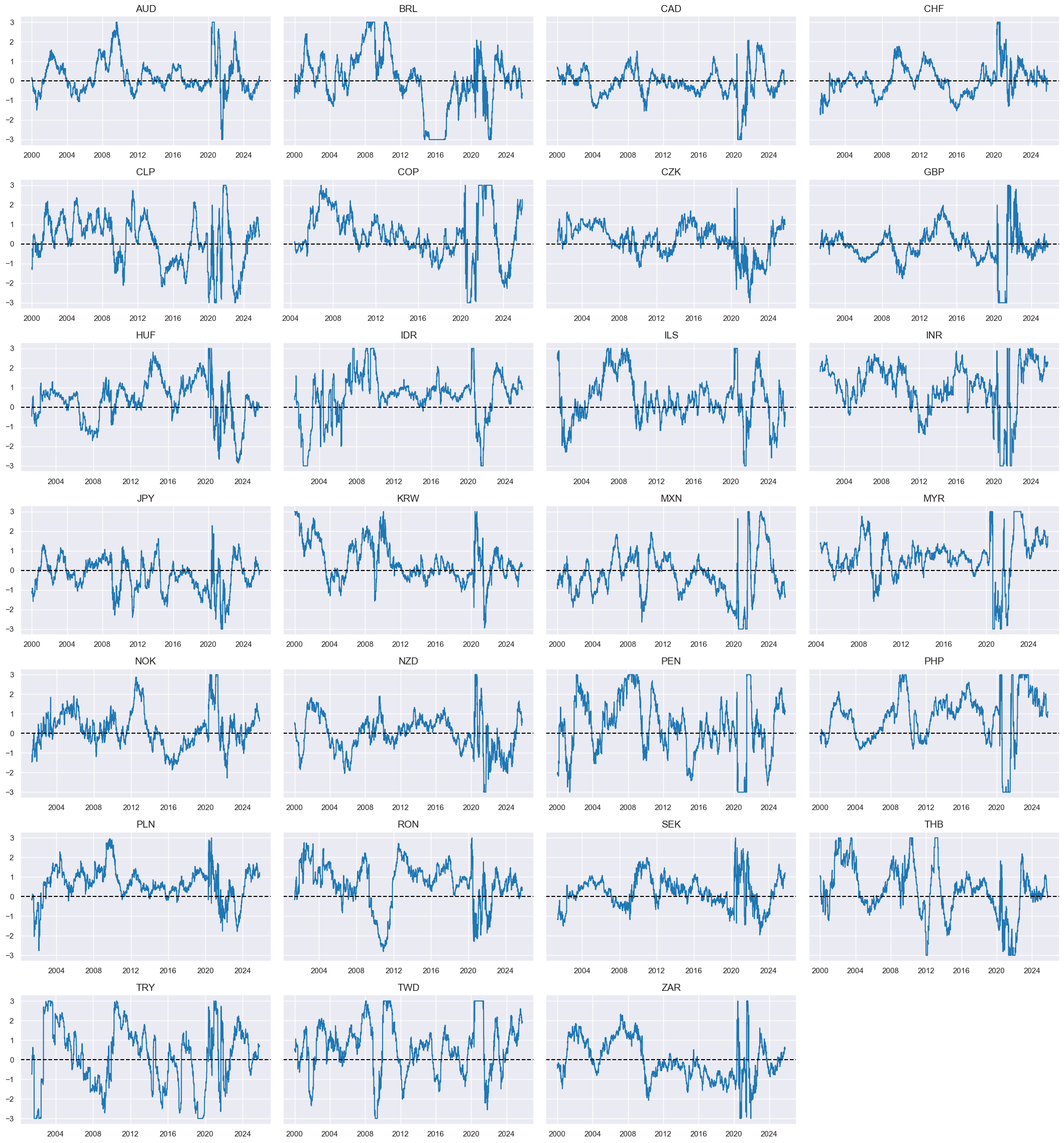
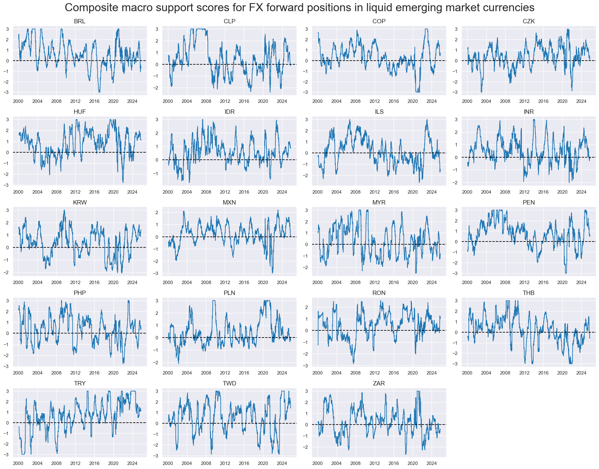
Composite macro support scores

# Weighted linear combinations
factz = [
    "XBTREND_ZN",
    "IITREND_ZN",
    "RGDPTREND_ZN",
    "RXINFTREND_ZN",
    "XEXPTREND_ZN",
]
xcatx = factz
sdate = "2000-01-01"
new_cat = "MACRO"
cidx = cids_fx

dfa = msp.linear_composite(
    dfx,
    xcats=xcatx,
    cids=cidx,
    complete_xcats=False,
    start=sdate,
    new_xcat=new_cat,
)
dfx = msm.update_df(dfx, dfa)

dfa = msp.make_zn_scores(
    dfx,
    xcat=new_cat,
    cids=cidx,
    sequential=True,
    min_obs=261 * 5,
    neutral="zero",
    pan_weight=1,
    thresh=3,
    postfix="_ZC",
    est_freq="m",
)
dfx = msm.update_df(dfx, dfa)

xcatx = ["MACRO_ZC"]
cidx = cids_emfx

msp.view_timelines(
    dfx,
    xcats=xcatx,
    cids=cidx,
    ncol=4,
    start="2000-01-01",
    same_y=False,
    title="Composite macro support scores for FX forward positions in liquid emerging market currencies",
    title_fontsize=26,
    height=2,
    size=(10, 10),
    all_xticks=True,
)

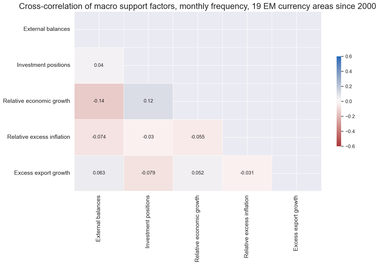
xcatx = factz

factz_labels = {
    "XBTREND_ZN": "External balances",
    "IITREND_ZN": "Investment positions",
    "RGDPTREND_ZN": "Relative economic growth",
    "RXINFTREND_ZN": "Relative excess inflation",
    "XEXPTREND_ZN": "Excess export growth",
}

msp.correl_matrix(
    dfx,
    xcats=xcatx,
    cids=cidx,
    freq="M",
    title="Cross-correlation of macro support factors, monthly frequency, 19 EM currency areas since 2000",
    title_fontsize=20,
    size=(13, 9),
    max_color=0.6,
    xcat_labels=factz_labels,
    show=True,
    annot=True
)

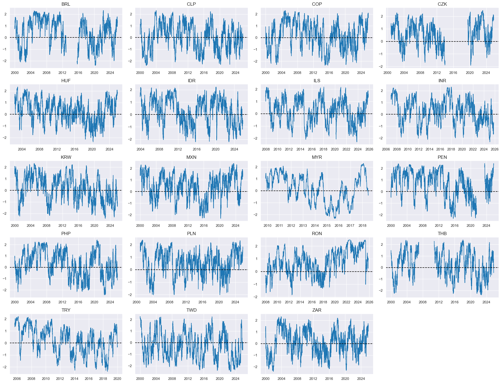
Trends

Robust trends

# Returns and adjustment scores

fxrs = ["FXXR_NSA"]

scoresz = [
    "XBTREND_ZN",
    "IITREND_ZN",
    "RGDPTREND_ZN",
    "RXINFTREND_ZN",
    "XEXPTREND_ZN",
    "MACRO_ZC",
]

# Creating a function that returns the cdf as dataframe
def norm_cdf_df(df):
    """Apply scipy.stats.norm.cdf to a DataFrame and return a DataFrame."""
    return pd.DataFrame(norm.cdf(df.values), index=df.index, columns=df.columns)

# T-stat trend following strategy (Tzotchev, D. (2018).

cidx = cids_fx
lookbacks = [32, 64, 126, 252, 504] # 1.5, 3, 6, 12, 24 months

calcs = []
for fxr in fxrs:
    
    signals = []
    for lb in lookbacks:
        mean_calc = f"{fxr}_MEAN_{lb} = {fxr}.rolling( {lb} ).mean( )"
        std_calc = f"{fxr}_STD_{lb} = {fxr}.rolling( {lb} ).std( ddof=1 )"
        tstat_calc = (
            f"{fxr}_TSTAT_{lb} = {fxr}_MEAN_{lb} / ( {fxr}_STD_{lb} / np.sqrt( {lb} ) )"
        )
        prob_calc = f"{fxr}_PROB_{lb} = norm_cdf_df( {fxr}_TSTAT_{lb} )"
        signal_calc = f"{fxr}_SIGNAL_{lb} = 2 * {fxr}_PROB_{lb} - 1"

        signals.append( f"{fxr}_SIGNAL_{lb}" )
        
        calcs += [mean_calc, std_calc, tstat_calc, prob_calc, signal_calc]

    composite_signal = f"{fxr}_RTS = ( {' + '.join(signals)} ) / {len(lookbacks)}"
    calcs.append(composite_signal)


# Calculate the signals
dfa = msp.panel_calculator(dfx, calcs, cids=cidx, blacklist=fxblack, external_func={"norm_cdf_df": norm_cdf_df})
dfx = msm.update_df(dfx, dfa)

# Rename trends for simplicity
dict_rename = {
    "FXXR_NSA_RTS": "ROBFXR_TREND",
    "FXNA_NSA_RTS": "ROBFNA_TREND",
}
dfx["xcat"] = dfx["xcat"].replace(dict_rename, regex=True)

# Composite signals names:
robtrends = ["ROBFXR_TREND"]

# Normalize trend signals sequentially (for modification)
xcatx = robtrends
cidx = cids_fx

for xc in xcatx:
    dfaa = msp.make_zn_scores(
        dfx,
        xcat=xc,
        cids=cidx,
        sequential=True,
        min_obs=522,  # oos scaling after 2 years of panel data
        est_freq="m",
        neutral="zero",
        pan_weight=1,
        thresh=3,
        postfix="Z",
    )
    dfa = msm.update_df(dfa, dfaa)

dfx = msm.update_df(dfx, dfa)

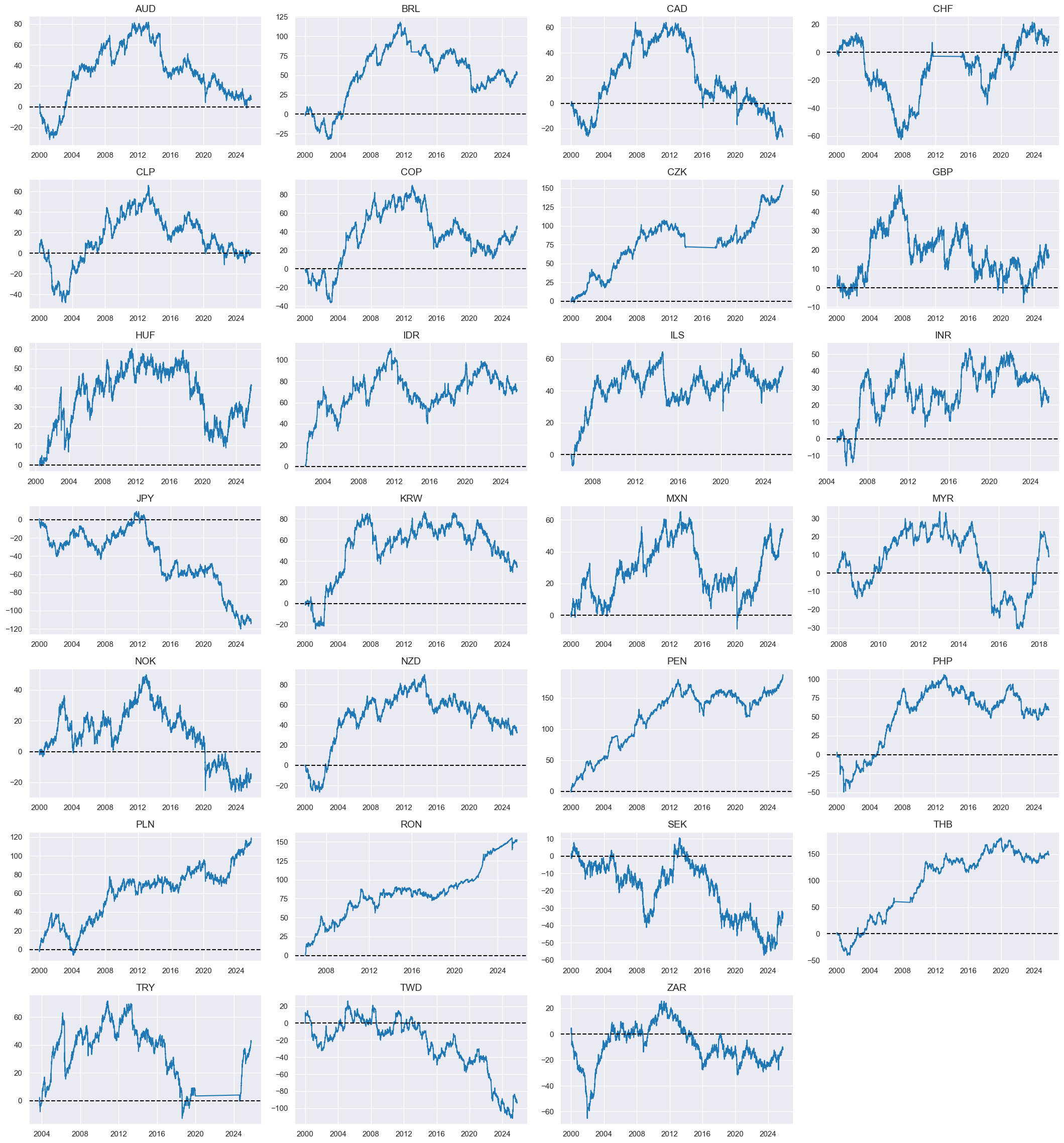
robtrends = [tr + "Z" for tr in robtrends]

xcatx = robtrends
cidx = cids_emfx

msp.view_timelines(
    dfx,
    xcats=xcatx,
    cids=cidx,
    ncol=4,
    start="2000-01-01",
    same_y=False,
    height=2.2,
    size=(10, 10),
    all_xticks=True,
)

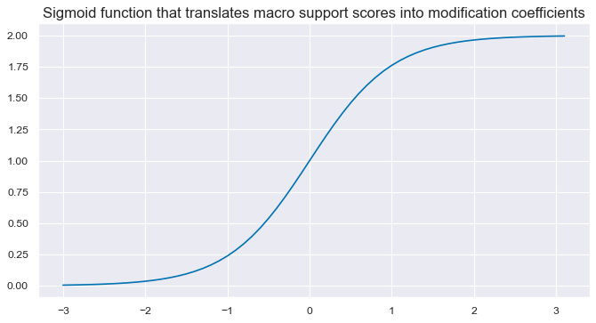
Modified robust trends

# Illustrate sigmoid function

def sigmoid(x):
    return 2 / (1 + np.exp(-2 * x))


ar = np.arange(-3, 3.2, 0.1)
plt.figure(figsize=(10, 5), dpi=80)
plt.plot(ar, sigmoid(ar))
plt.title(
    "Sigmoid function that translates macro support scores into modification coefficients",
    fontsize=15,
)
plt.show()

# Calculate general modification coefficients (independent of sign)

calcs = []

for zd in scoresz:
    calcs += [f"{zd}_C = ( {zd} ).applymap( lambda x: 2 / (1 + np.exp( - 2 * x)) ) "]
dfa = msp.panel_calculator(dfx, calcs=calcs, cids=cidx)
dfx = msm.update_df(dfx, dfa)

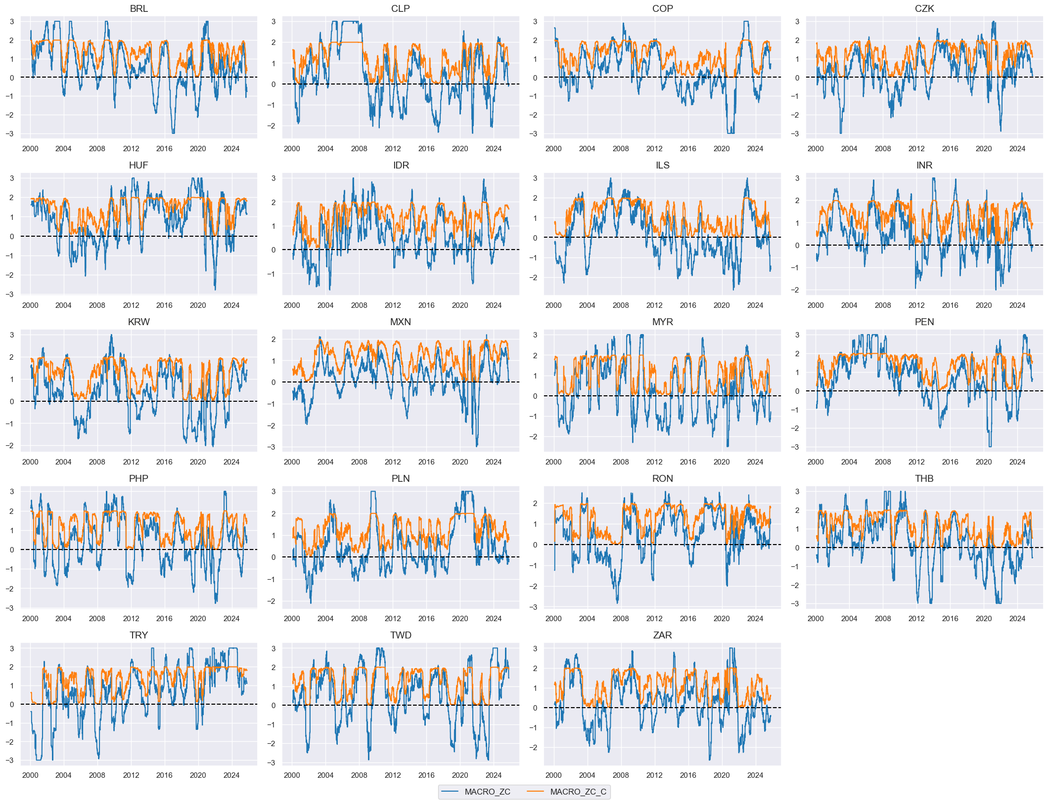
# Visualize general modification coefficients

xcatx = ["MACRO_ZC", "MACRO_ZC_C"]
cidx = cids_emfx

msp.view_timelines(
    dfx,
    xcats=xcatx,
    cids=cidx,
    ncol=4,
    start="2000-01-01",
    same_y=False,
    height=2.2,
    size=(10, 10),
    all_xticks=True,
)

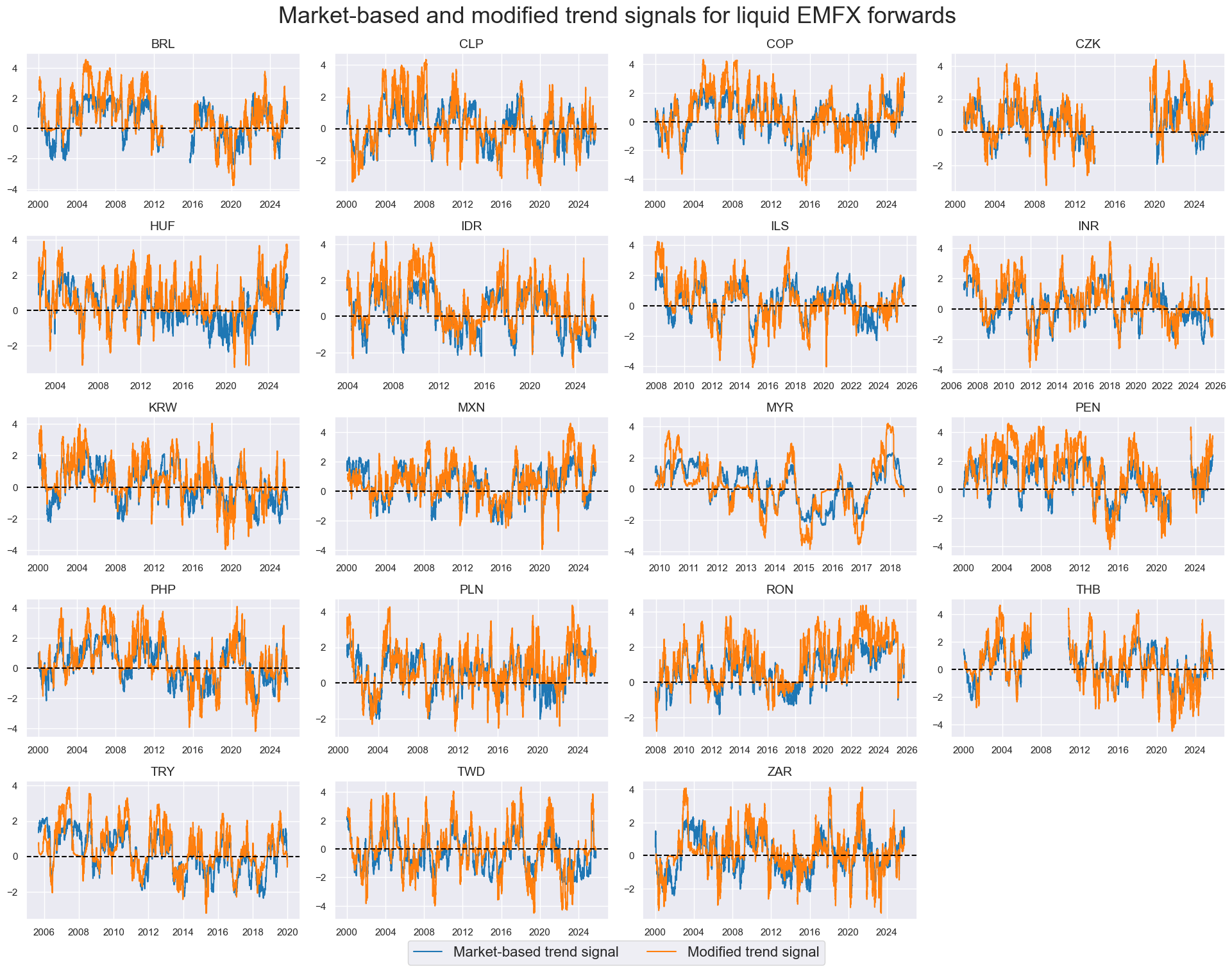
# Modified robust trends based on sign-dependent modification

calcs = []
for tr in robtrends:
    for xs in scoresz:
        trxs = tr + "m" + xs.split("_")[0]
        calcs += [f"{trxs}_C = (1 - np.sign( {tr} )) + np.sign( {tr} ) * {xs}_C"]
        calcs += [f"{trxs} = {trxs}_C * {tr}"]

dfa = msp.panel_calculator(dfx, calcs=calcs, cids=cids_fx, blacklist=fxblack)
dfx = msm.update_df(dfx, dfa)

rob_trends_mod = [xc for xc in dfa["xcat"].unique() if not xc.endswith("_C")]

xcatx = ["ROBFXR_TRENDZ", "ROBFXR_TRENDZmMACRO"]
cidx = cids_emfx

dict_labs = {
    "ROBFXR_TRENDZ": "Market-based trend signal",
    "ROBFXR_TRENDZmMACRO": "Modified trend signal",
}

msp.view_timelines(
    dfx,
    xcats=xcatx,
    cids=cidx,
    ncol=4,
    start="2000-01-01",
    same_y=False,
    title="Market-based and modified trend signals for liquid EMFX forwards",
    title_fontsize=26,
    height=2,
    size=(8, 8),
    all_xticks=True,
    xcat_labels=dict_labs,
    legend_fontsize=16,
)

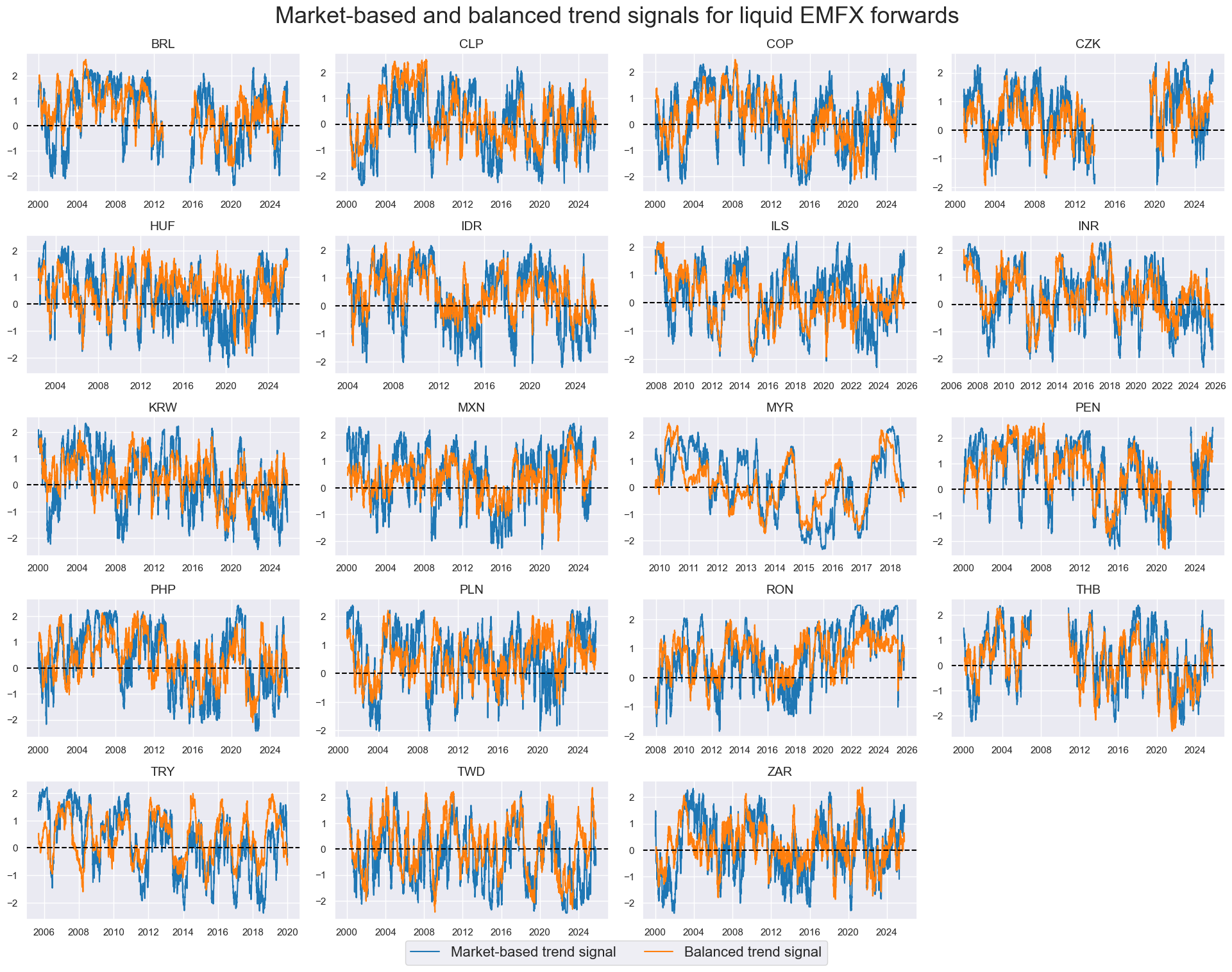
Balanced robust trends

# Balanced robust trend calculation

calcs = []
for tr in robtrends:
    for xs in scoresz:
        trxs = tr + "b" + xs.split("_")[0]
        calcs += [f"{trxs} = ( {tr} + ( {xs} ) ) / 2"]

dfa = msp.panel_calculator(dfx, calcs=calcs, cids=cids_fx, blacklist=fxblack)
dfx = msm.update_df(dfx, dfa)

rob_trends_bal = [xc for xc in dfa["xcat"].unique() if not xc.endswith("_C")]

xcatx = ["ROBFXR_TRENDZ", "ROBFXR_TRENDZbMACRO"]
cidx = cids_emfx

dict_labs = {
    "ROBFXR_TRENDZ": "Market-based trend signal",
    "ROBFXR_TRENDZbMACRO": "Balanced trend signal",
}

msp.view_timelines(
    dfx,
    xcats=xcatx,
    cids=cidx,
    ncol=4,
    start="2000-01-01",
    same_y=False,
    title="Market-based and balanced trend signals for liquid EMFX forwards",
    title_fontsize=26,
    height=2,
    size=(8, 8),
    all_xticks=True,
    xcat_labels=dict_labs,
    legend_fontsize=16,
)

Targets

Directional vol-targeted returns

xcatx = ["FXXR_VT10"]
cidx = cids_fx

msp.view_timelines(
    dfx,
    xcats=xcatx,
    cids=cidx,
    ncol=4,
    cumsum=True,
    start="2000-01-01",
    same_y=False,
    height=2.2,
    size=(10, 10),
    all_xticks=True,
    blacklist=fxblack,
)

Value checks

Specs and panel test

sigs = [
    "ROBFXR_TRENDZ",
    "ROBFXR_TRENDZmMACRO",
    "ROBFXR_TRENDZbMACRO",
]

targ = "FXXR_VT10"
cidx = cids_emfx

dict_rob = {
    "sigs": sigs,
    "targ": targ,
    "cidx": cidx,
    "black": fxblack,
    "srr": None,
    "pnls": None,
}

dix = dict_rob

sigs = dix["sigs"]
targ = dix["targ"]
cidx = dix["cidx"]
blax = dix["black"]

# Dictionary to store CategoryRelations objects
crx = []

# Create CategoryRelations objects for all signals
for sig in sigs:
    crx.append(
        msp.CategoryRelations(
        dfx,
        xcats=[sig, targ],
        cids=cidx,
        freq="M",
        lag=1,
        xcat_aggs=["last", "sum"],
        start="2000-01-01",
        blacklist=blax,
        xcat_trims=[None, None],
        )
    )

# Display scatter plots for all signals
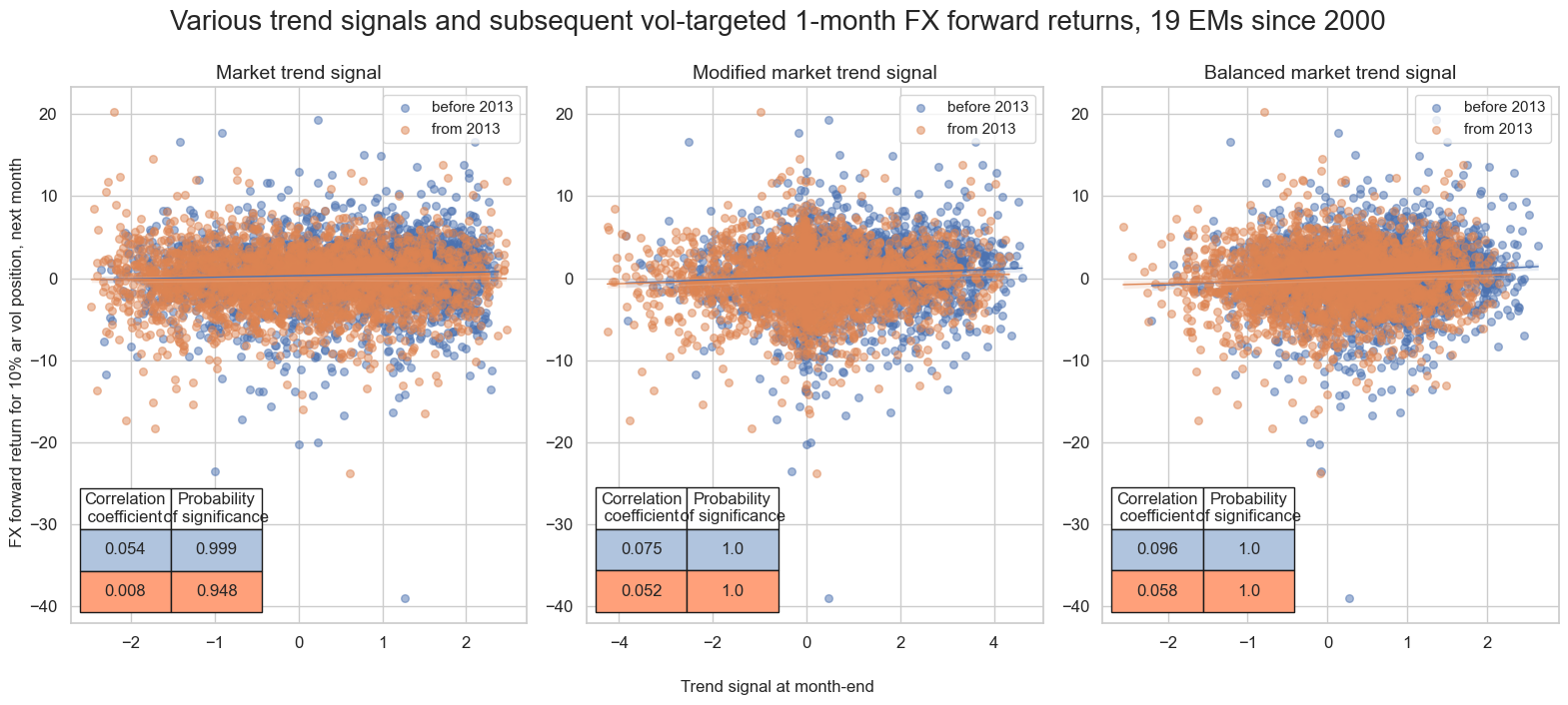
msv.multiple_reg_scatter(
    cat_rels=crx,
    coef_box="lower left",
    ncol=3,
    nrow=1,
    separator=2013,
    xlab="Trend signal at month-end",
    ylab="FX forward return for 10% ar vol position, next month",
    title="Various trend signals and subsequent vol-targeted 1-month FX forward returns, 19 EMs since 2000",
    title_fontsize=20,
    figsize=(16, 7),
    prob_est="map",
    subplot_titles=["Market trend signal", "Modified market trend signal", "Balanced market trend signal"],
    share_axes=False,
)

Accuracy and correlation check

dix = dict_rob

sigs = dix["sigs"]
targ = dix["targ"]
cidx = dix["cidx"]
blax = dix["black"]

srr = mss.SignalReturnRelations(
    dfx,
    cids=cidx,
    sigs=sigs,
    rets=targ,
    freqs="M",
    start="2000-01-01",
    blacklist=blax,
)

dix["srr"] = srr

dix = dict_rob
srrx = dix["srr"]
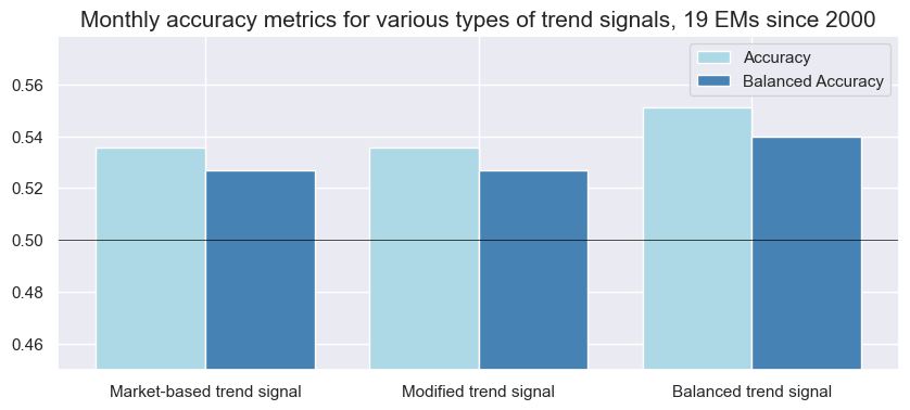
display(srrx.multiple_relations_table().round(3))

dict_labs = {
    "ROBFXR_TRENDZ": "Market-based trend signal",
    "ROBFXR_TRENDZmMACRO": "Modified trend signal",
    "ROBFXR_TRENDZbMACRO": "Balanced trend signal",
}

srrx.accuracy_bars(type="signals", 
                  title="Monthly accuracy metrics for various types of trend signals, 19 EMs since 2000", 
                  freq="m",
                  size=(10, 4),
                  title_fontsize=15,
                  x_labels=dict_labs
                  )

				accuracy	bal_accuracy	pos_sigr	pos_retr	pos_prec	neg_prec	pearson	pearson_pval	kendall	kendall_pval	auc
Return	Signal	Frequency	Aggregation
FXXR_VT10	ROBFXR_TRENDZ	M	last	0.536	0.527	0.607	0.547	0.568	0.485	0.043	0.002	0.035	0.0	0.526
	ROBFXR_TRENDZbMACRO	M	last	0.551	0.540	0.667	0.547	0.574	0.506	0.089	0.000	0.060	0.0	0.536
	ROBFXR_TRENDZmMACRO	M	last	0.536	0.527	0.607	0.547	0.568	0.485	0.076	0.000	0.049	0.0	0.526

Naive PnL

dix = dict_rob

sigx = dix["sigs"]
targ = dix["targ"]
cidx = dix["cidx"]
blax = dix["black"]

naive_pnl = msn.NaivePnL(
    dfx,
    ret=targ,
    sigs=sigx,
    cids=cidx,
    start="2000-01-01",
    blacklist=blax,
    bms=["USD_EQXR_NSA"],
)

for sig in sigx:
    naive_pnl.make_pnl(
        sig,
        sig_neg=False,
        sig_op="raw",
        thresh=5,
        rebal_freq="daily",
        vol_scale=10,
        rebal_slip=1,
        pnl_name=sig + "_PZN",
    )


naive_pnl.make_long_pnl(vol_scale=10, label="Long only")
dix["pnls"] = naive_pnl

dix = dict_rob

sigx = dix["sigs"]
cidx = dix["cidx"]
naive_pnl = dix["pnls"]
pnls = [sig + "_PZN" for sig in sigx] + ["Long only"]

dict_labs = {
    "ROBFXR_TRENDZ_PZN": "Market-based trend signal",
    "ROBFXR_TRENDZmMACRO_PZN": "Modified trend signal",
    "ROBFXR_TRENDZbMACRO_PZN": "Balanced trend signal",
    "Long only": "Long-only risk parity",
}

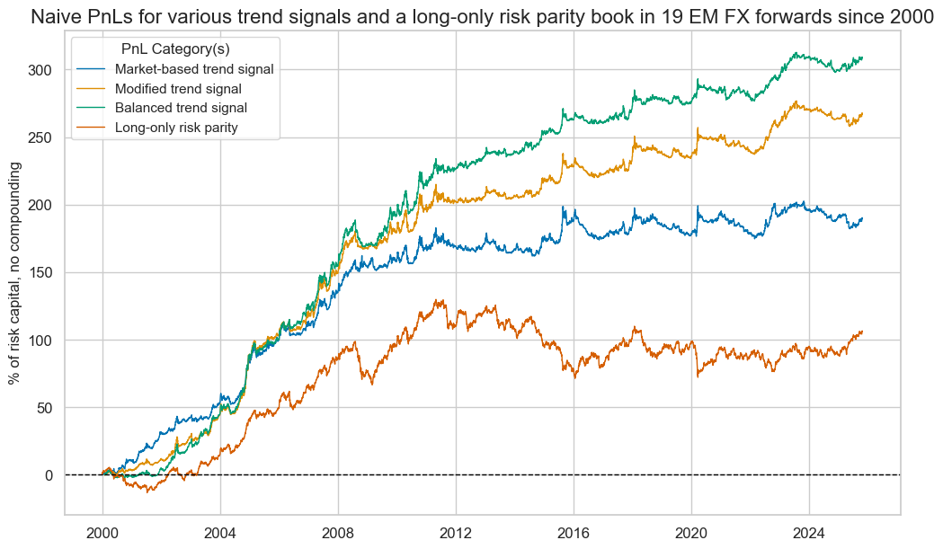
naive_pnl.plot_pnls(
    pnl_cats=pnls,
    pnl_cids=["ALL"],
    start="2000-01-01",
    title="Naive PnLs for various trend signals and a long-only risk parity book in 19 EM FX forwards since 2000",
    title_fontsize=16,
    xcat_labels=dict_labs,
    figsize=(12, 7),
)

df_eval = naive_pnl.evaluate_pnls(
    pnl_cats=pnls,
    pnl_cids=["ALL"],
    start="2000-01-01",
)
display(df_eval.transpose().astype("float").round(2))

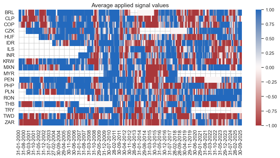
naive_pnl.signal_heatmap(
    pnl_name='ROBFXR_TRENDZ_PZN',
    pnl_cids=cidx,
    freq="m",
    start="2000-01-01",
    figsize=(12, 6)
)

naive_pnl.signal_heatmap(
    pnl_name='ROBFXR_TRENDZbMACRO_PZN',
    pnl_cids=cidx,
    freq="m",
    start="2020-01-01",
    figsize=(12, 6)
)

	Return %	St. Dev. %	Sharpe Ratio	Sortino Ratio	Max 21-Day Draw %	Max 6-Month Draw %	Peak to Trough Draw %	Top 5% Monthly PnL Share	USD_EQXR_NSA correl	Traded Months
xcat
ROBFXR_TRENDZ_PZN	7.35	10.0	0.73	1.04	-12.73	-18.51	-24.88	0.76	-0.03	310.0
ROBFXR_TRENDZmMACRO_PZN	10.38	10.0	1.04	1.49	-16.03	-12.57	-19.85	0.61	0.04	310.0
ROBFXR_TRENDZbMACRO_PZN	11.99	10.0	1.20	1.73	-17.40	-17.71	-19.91	0.51	0.08	310.0
Long only	4.10	10.0	0.41	0.56	-21.26	-26.00	-58.50	1.08	0.32	310.0

Naive PnL of binary strategy

dix = dict_rob

sigx = dix["sigs"]
targ = dix["targ"]
cidx = dix["cidx"]
blax = dix["black"]

naive_pnl = msn.NaivePnL(
    dfx,
    ret=targ,
    sigs=sigx,
    cids=cidx,
    start="2000-01-01",
    blacklist=blax,
    bms=["USD_EQXR_NSA"],
)

for sig in sigx:
    naive_pnl.make_pnl(
        sig,
        sig_neg=False,
        sig_op="binary",
        entry_barrier=1.0,
        exit_barrier=0.25,
        rebal_freq="daily",
        vol_scale=10,
        rebal_slip=1,
        pnl_name=sig + "_BIN",
    )


naive_pnl.make_long_pnl(vol_scale=10, label="Long only")
dix["pnls2"] = naive_pnl

dix = dict_rob

sigx = dix["sigs"]
cidx = dix["cidx"]
naive_pnl = dix["pnls2"]
pnls = [sig + "_BIN" for sig in sigx] + ["Long only"]

dict_labs = {
    "ROBFXR_TRENDZ_BIN": "Binary market trend signal",
    "ROBFXR_TRENDZmMACRO_BIN": "Binary modified trend signal",
    "ROBFXR_TRENDZbMACRO_BIN": "Binary balanced trend signal",
    "Long only": "Long-only risk parity",
}

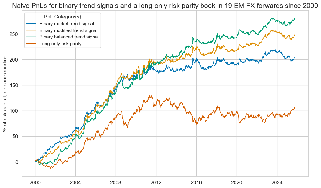
naive_pnl.plot_pnls(
    pnl_cats=pnls,
    pnl_cids=["ALL"],
    start="2000-01-01",
    title="Naive PnLs for binary trend signals and a long-only risk parity book in 19 EM FX forwards since 2000",
    title_fontsize=16,
    xcat_labels=dict_labs,
    figsize=(12, 7),
)

df_eval = naive_pnl.evaluate_pnls(
    pnl_cats=pnls,
    pnl_cids=["ALL"],
    start="2000-01-01",
)
display(df_eval.transpose().astype("float").round(2))

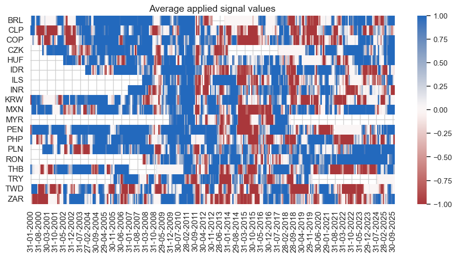
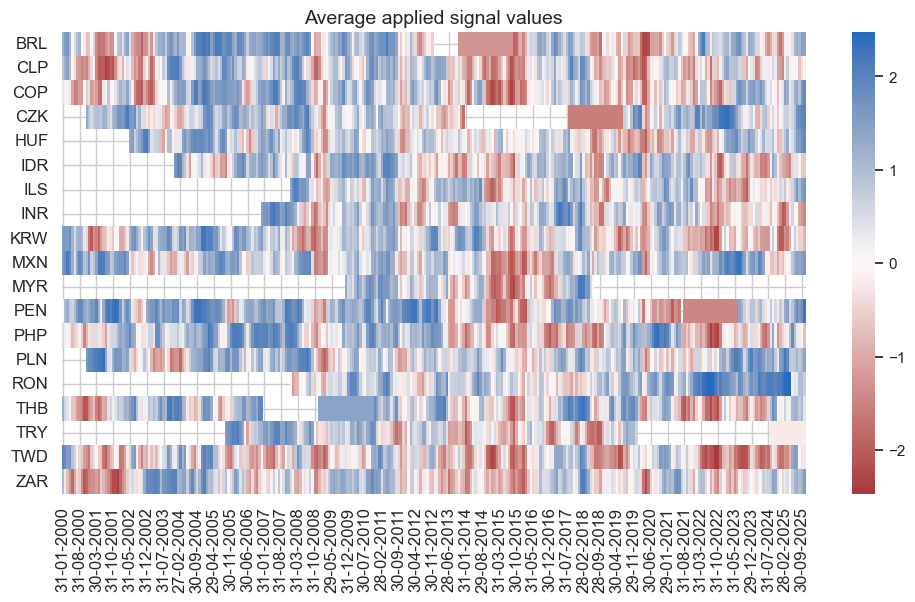
naive_pnl.signal_heatmap(
    pnl_name='ROBFXR_TRENDZ_BIN',
    pnl_cids=cidx,
    freq="m",
    start="2000-01-01",
    figsize=(12, 5)
)

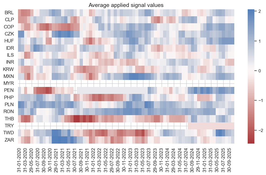
naive_pnl.signal_heatmap(
    pnl_name='ROBFXR_TRENDZmMACRO_BIN',
    pnl_cids=cidx,
    freq="m",
    start="2000-01-01",
    figsize=(12, 5)
)

	Return %	St. Dev. %	Sharpe Ratio	Sortino Ratio	Max 21-Day Draw %	Max 6-Month Draw %	Peak to Trough Draw %	Top 5% Monthly PnL Share	USD_EQXR_NSA correl	Traded Months
xcat
ROBFXR_TRENDZ_BIN	7.93	10.0	0.79	1.13	-14.70	-21.23	-25.36	0.62	-0.01	310.0
ROBFXR_TRENDZmMACRO_BIN	9.63	10.0	0.96	1.38	-16.82	-17.74	-20.91	0.54	0.03	310.0
ROBFXR_TRENDZbMACRO_BIN	10.81	10.0	1.08	1.56	-16.73	-21.16	-23.73	0.49	0.08	310.0
Long only	4.10	10.0	0.41	0.56	-21.26	-26.00	-58.50	1.08	0.32	310.0