Check out JPMaQS #
This notebook demonstrates how to download JPMaQS data using the
macrosynergy
package, a specialized library for macro quantamental research, and perform some basic transformation and analysis, using the popular
pandas
library.
Import Packages & JPMaQS data access #
JPMaQS data is accessed using the
JPMaQSDownload
class in the
macrosynergy.download
subpackage. This wraps around the
DataQuery API
.
For more information see here or use the free dataset on Kaggle .
# Uncomment below if running on Kaggle
"""
%%capture
! pip install macrosynergy --upgrade"""

import numpy as np
import pandas as pd
import matplotlib as mpl
import matplotlib.pyplot as plt
import seaborn as sns
from macrosynergy.download import JPMaQSDownload
import os

import warnings
warnings.simplefilter("ignore")
Each time series in JPMaQS is uniquely identified by a ticker, formed as:
<cid>_<xcat>
e.g.
USD_CPIC_SJA_P6M6ML6AR
with
-
Cross-sections (
cid): typically country or currency codes (e.g.,USD,EUR) -
Data categories (
xcat): macro or market indicator types (e.g., inflation, credit, returns)
Each ticker includes one or more metrics, such as:
-
value: indicator value -
eop_lag,mop_lag: lag between observation and release dates -
grade: data quality (1 to 3)
Focus of this notebook: countries with active interest rate swap (IRS) markets.
Full definitions of xcat codes can be found on the Macro Quantamental Academy , JPMorgan Markets (with login), or Kaggle (for the demo dataset).
# List of cross-sections
cids_dm = ["AUD", "CAD", "CHF", "EUR", "GBP", "JPY", "NOK", "NZD", "SEK", "USD"]
cids_em = [
    "CLP",
    "COP",
    "CZK",
    "HUF",
    "IDR",
    "ILS",
    "INR",
    "KRW",
    "MXN",
    "PLN",
    "THB",
    "TRY",
    "TWD",
    "ZAR"
]
cids = cids_dm + cids_em

# Main quantamental and return categories
macro_xcats = [
    # Inflation
    "CPIC_SA_P1M1ML12",
    "CPIC_SJA_P3M3ML3AR",
    "CPIC_SJA_P6M6ML6AR",
    "CPIH_SA_P1M1ML12",
    "CPIH_SJA_P3M3ML3AR",
    "CPIH_SJA_P6M6ML6AR",
    "INFTEFF_NSA",
    # Growth
    "INTRGDP_NSA_P1M1ML12_3MMA",
    "INTRGDPv5Y_NSA_P1M1ML12_3MMA",
    "RGDP_SA_P1Q1QL4_20QMA",
    # Interest rates
    "RYLDIRS02Y_NSA",
    "RYLDIRS05Y_NSA",
    # Private credit
    "PCREDITGDP_SJA_D1M1ML12",
    "PCREDITBN_SJA_P1M1ML12",
]

return_xcats = [
    # Interest rate swaps
    "DU02YXR_NSA",
    "DU05YXR_NSA",
    "DU02YXR_VT10",
    "DU05YXR_VT10",
    # Equity index futures
    "EQXR_NSA",
    "EQXR_VT10",
    # FX forwards
    "FXXR_NSA",
    "FXXR_VT10",
]

xcats = macro_xcats + return_xcats
The
download
method of
JPMaQSDownload
accepts a list of tickers, which we generate using all combinations of
cids
and
xcats
defined above.
Credentials are required and it is recommended to store these as secure environment variables.
# Uncomment if running on Kaggle
"""for dirname, _, filenames in os.walk('/kaggle/input'):
    for filename in filenames:
        print(os.path.join(dirname, filename))

df = pd.read_csv('../input/fixed-income-returns-and-macro-trends/JPMaQS_Quantamental_Indicators.csv', index_col=0, parse_dates=['real_date'])"""

# Comment below if running on Kaggle
start_date = "2000-01-01"
tickers = [f"{cid}_{xcat}" for cid in cids for xcat in xcats]

client_id: str = os.getenv("DQ_CLIENT_ID")
client_secret: str = os.getenv("DQ_CLIENT_SECRET")

with JPMaQSDownload(client_id=client_id, client_secret=client_secret) as dq:
    df = dq.download(
        tickers=tickers,
        start_date=start_date,
        metrics=["value"],
        show_progress=True,
    )
Downloading data from JPMaQS.
Timestamp UTC:  2025-07-23 11:58:46
Connection successful!
Requesting data: 100%|██████████| 27/27 [00:05<00:00,  4.92it/s]
Downloading data: 100%|██████████| 27/27 [00:16<00:00,  1.67it/s]
Some expressions are missing from the downloaded data. Check logger output for complete list.
18 out of 528 expressions are missing. To download the catalogue of all available expressions and filter the unavailable expressions, set `get_catalogue=True` in the call to `JPMaQSDownload.download()`.
Handling JPMaQS dataframes #
The downloaded JPMaQS dataset is a standard long-format DataFrame with four key columns:
real_date
,
cid
,
xcat
, and
value
.
An example can be seen below.
df
| real_date | cid | xcat | value | |
|---|---|---|---|---|
| 0 | 2001-07-04 | AUD | DU05YXR_VT10 | -0.233174 |
| 1 | 2001-07-05 | AUD | DU05YXR_VT10 | 0.651543 |
| 2 | 2001-07-06 | AUD | DU05YXR_VT10 | 0.012344 |
| 3 | 2001-07-09 | AUD | DU05YXR_VT10 | 0.406206 |
| 4 | 2001-07-10 | AUD | DU05YXR_VT10 | -0.037190 |
| ... | ... | ... | ... | ... |
| 3180467 | 2025-07-16 | ZAR | RYLDIRS05Y_NSA | 3.032594 |
| 3180468 | 2025-07-17 | ZAR | RYLDIRS05Y_NSA | 3.097594 |
| 3180469 | 2025-07-18 | ZAR | RYLDIRS05Y_NSA | 3.062594 |
| 3180470 | 2025-07-21 | ZAR | RYLDIRS05Y_NSA | 3.082594 |
| 3180471 | 2025-07-22 | ZAR | RYLDIRS05Y_NSA | 2.997594 |
3180472 rows × 4 columns
Standard
pandas
and
matplotlib
operations can be performed on the standard JPMaQS dataframe, such as those for visualization and transformation.
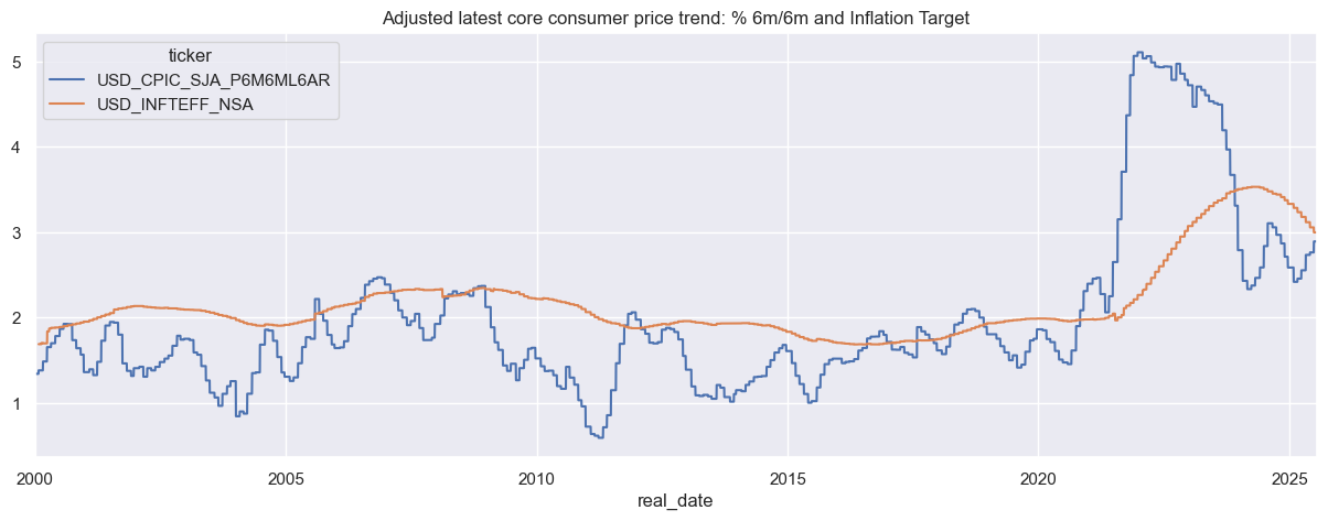
# Get 6m/6m core inflation and inflation target for the US
dfx = df[
    df.xcat.isin(['CPIC_SJA_P6M6ML6AR', 'INFTEFF_NSA']) &
    (df.cid == "USD")
]

# Pivot to wide format
dfx["ticker"] = dfx["cid"] + "_" + dfx["xcat"]
dfw = dfx.pivot_table(index="real_date", columns="ticker", values="value").replace(0, np.nan)

# Plot
sns.set(rc={"figure.figsize": (15, 5)})
dfw.plot(title="Adjusted latest core consumer price trend: % 6m/6m and Inflation Target")
plt.show()
Summary statistics #
# Get inflation and growth statistics for 4 different countries
xcatx = ["CPIC_SJA_P6M6ML6AR", "INTRGDPv5Y_NSA_P1M1ML12_3MMA"]
cidx = cids_dm[2:6]
dfx = df[df["xcat"].isin(xcatx) & df["cid"].isin(cidx)]

# Simplify xcat names for ease
nicknames = {"CPIC_SJA_P6M6ML6AR": "CORE_CPI_TREND","INTRGDPv5Y_NSA_P1M1ML12_3MMA": "GDP_TREND"}
dfx["xcat"] = dfx["xcat"].map(nicknames)

# Pivot to wide format
dfx["ticker"] = dfx["cid"] + "_" + dfx["xcat"]
dfw = dfx.pivot_table(index="real_date", columns="ticker", values="value").replace(0, np.nan)

# Check out double category panel
print("Inflation and growth dataframe summary:\n")
print(dfw.info())

print("\nFirst 5 rows:")
display(dfw.head())
Inflation and growth dataframe summary:

<class 'pandas.core.frame.DataFrame'>
DatetimeIndex: 6667 entries, 2000-01-03 to 2025-07-22
Data columns (total 8 columns):
 #   Column              Non-Null Count  Dtype
---  ------              --------------  -----
 0   CHF_CORE_CPI_TREND  5802 non-null   float64
 1   CHF_GDP_TREND       6667 non-null   float64
 2   EUR_CORE_CPI_TREND  6650 non-null   float64
 3   EUR_GDP_TREND       6321 non-null   float64
 4   GBP_CORE_CPI_TREND  6667 non-null   float64
 5   GBP_GDP_TREND       6667 non-null   float64
 6   JPY_CORE_CPI_TREND  5235 non-null   float64
 7   JPY_GDP_TREND       6667 non-null   float64
dtypes: float64(8)
memory usage: 468.8 KB
None

First 5 rows:
| ticker | CHF_CORE_CPI_TREND | CHF_GDP_TREND | EUR_CORE_CPI_TREND | EUR_GDP_TREND | GBP_CORE_CPI_TREND | GBP_GDP_TREND | JPY_CORE_CPI_TREND | JPY_GDP_TREND |
|---|---|---|---|---|---|---|---|---|
| real_date | ||||||||
| 2000-01-03 | NaN | 0.381352 | NaN | NaN | 0.314695 | -0.283961 | NaN | -0.407442 |
| 2000-01-04 | NaN | 0.381352 | NaN | NaN | 0.314695 | -0.283961 | NaN | -0.407442 |
| 2000-01-05 | NaN | 0.381352 | NaN | NaN | 0.314695 | -0.283961 | NaN | -0.407442 |
| 2000-01-06 | NaN | 0.381352 | NaN | NaN | 0.314695 | -0.283961 | NaN | -0.407442 |
| 2000-01-07 | NaN | 0.347481 | NaN | NaN | 0.314695 | -0.283961 | NaN | -0.407442 |
# Mean and standard deviation
dfw.aggregate(["mean", "std"])
| ticker | CHF_CORE_CPI_TREND | CHF_GDP_TREND | EUR_CORE_CPI_TREND | EUR_GDP_TREND | GBP_CORE_CPI_TREND | GBP_GDP_TREND | JPY_CORE_CPI_TREND | JPY_GDP_TREND |
|---|---|---|---|---|---|---|---|---|
| mean | 0.443162 | -0.289337 | 1.629545 | -0.479751 | 2.185978 | -0.641548 | 0.675772 | 0.030875 |
| std | 0.780606 | 1.615642 | 1.037796 | 2.493975 | 1.406263 | 3.241864 | 1.419324 | 2.206299 |
# Summary stats from March 2020 to March 2021
dfw.loc["2020-03":"2021-03"].agg(["mean", "max", "min"])
| ticker | CHF_CORE_CPI_TREND | CHF_GDP_TREND | EUR_CORE_CPI_TREND | EUR_GDP_TREND | GBP_CORE_CPI_TREND | GBP_GDP_TREND | JPY_CORE_CPI_TREND | JPY_GDP_TREND |
|---|---|---|---|---|---|---|---|---|
| mean | -0.052870 | -2.791305 | 0.915864 | -6.486250 | 2.035952 | -10.043104 | -0.100639 | -4.085330 |
| max | 0.451175 | -0.188694 | 1.410560 | -0.897233 | 3.289897 | -0.655196 | 0.834353 | -0.529565 |
| min | -0.824449 | -8.404835 | -0.201780 | -12.695249 | 1.309598 | -22.994717 | -1.140706 | -8.702678 |
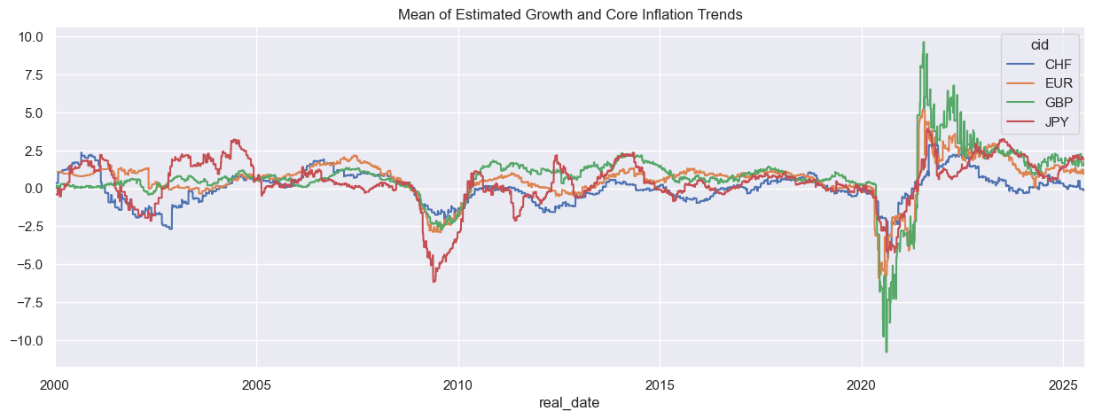
Applying mathematical operations #
JPMaQS time series panels with aligned columns and overlapping dates can be combined using standard mathematical operations.
# Convert to wide format
dfx_pivot = dfx.pivot(index = ["cid", "real_date"], columns="xcat",values="value")

# Calculate mean
dfx_pivot["CPI_GDP_MEAN"] = dfx_pivot.mean(axis = 1)

# Plot
dfx_pivot.unstack(0)["CPI_GDP_MEAN"].plot(figsize=(15, 5), title="Mean of Estimated Growth and Core Inflation Trends")
plt.show()
Wide format
pandas
dataframes can be melted back into long-format dataframes and standard JPMaQS quantamental dataframes.
# Melt dataframe
dfx_mean = dfx_pivot.iloc[:,-1:].reset_index().melt(id_vars=["cid", "real_date"])

# dfx has a ticker column, so add ticker column and add CPI_GDP_MEAN to dfx
dfx_mean["ticker"] = dfx_mean["cid"] + "_" + dfx_mean["xcat"]
dfx_new = pd.concat([dfx, dfx_mean], axis=0, ignore_index=True)
dfx_new
| real_date | cid | xcat | value | ticker | |
|---|---|---|---|---|---|
| 0 | 2000-01-03 | CHF | GDP_TREND | 0.381352 | CHF_GDP_TREND |
| 1 | 2000-01-04 | CHF | GDP_TREND | 0.381352 | CHF_GDP_TREND |
| 2 | 2000-01-05 | CHF | GDP_TREND | 0.381352 | CHF_GDP_TREND |
| 3 | 2000-01-06 | CHF | GDP_TREND | 0.381352 | CHF_GDP_TREND |
| 4 | 2000-01-07 | CHF | GDP_TREND | 0.347481 | CHF_GDP_TREND |
| ... | ... | ... | ... | ... | ... |
| 77412 | 2025-07-16 | JPY | CPI_GDP_MEAN | 1.894238 | JPY_CPI_GDP_MEAN |
| 77413 | 2025-07-17 | JPY | CPI_GDP_MEAN | 1.894238 | JPY_CPI_GDP_MEAN |
| 77414 | 2025-07-18 | JPY | CPI_GDP_MEAN | 1.889408 | JPY_CPI_GDP_MEAN |
| 77415 | 2025-07-21 | JPY | CPI_GDP_MEAN | 1.889408 | JPY_CPI_GDP_MEAN |
| 77416 | 2025-07-22 | JPY | CPI_GDP_MEAN | 1.889408 | JPY_CPI_GDP_MEAN |
77417 rows × 5 columns
Applying time series transformations #
JPMaQS tickers can be resampled to different frequencies for analysis.
# Select European and British GDP and inflation statistics
xcatx = ["INTRGDPv5Y_NSA_P1M1ML12_3MMA", "INTRGDPv10Y_NSA_P1M1ML12_3MMA", "CPIC_SJA_P6M6ML6AR"]
cidx = ["EUR", "GBP"]

dfx = df[df["xcat"].isin(xcatx) & df["cid"].isin(cidx)]

# Resample to get the last value of each month
dfx_monthly = (
    dfx.groupby(["cid", "xcat"])
    .resample("M", on="real_date")
    .last()["value"]
    .reset_index()
)
dfx_monthly
| cid | xcat | real_date | value | |
|---|---|---|---|---|
| 0 | EUR | CPIC_SJA_P6M6ML6AR | 2000-01-31 | 1.093003 |
| 1 | EUR | CPIC_SJA_P6M6ML6AR | 2000-02-29 | 1.042372 |
| 2 | EUR | CPIC_SJA_P6M6ML6AR | 2000-03-31 | 0.975460 |
| 3 | EUR | CPIC_SJA_P6M6ML6AR | 2000-04-30 | 0.976060 |
| 4 | EUR | CPIC_SJA_P6M6ML6AR | 2000-05-31 | 0.959466 |
| ... | ... | ... | ... | ... |
| 1207 | GBP | INTRGDPv5Y_NSA_P1M1ML12_3MMA | 2025-03-31 | 0.422620 |
| 1208 | GBP | INTRGDPv5Y_NSA_P1M1ML12_3MMA | 2025-04-30 | 0.651798 |
| 1209 | GBP | INTRGDPv5Y_NSA_P1M1ML12_3MMA | 2025-05-31 | 0.952007 |
| 1210 | GBP | INTRGDPv5Y_NSA_P1M1ML12_3MMA | 2025-06-30 | -0.475910 |
| 1211 | GBP | INTRGDPv5Y_NSA_P1M1ML12_3MMA | 2025-07-31 | -0.071961 |
1212 rows × 4 columns
Lagging, differencing and percentage changes are common time series transformations.
-
Macro factors are often lagged to study their impact on next-period market returns.
dfx_monthly_shift = dfx_monthly.copy()
dfx_monthly_shift["value"] = dfx_monthly_shift.groupby(["cid", "xcat"])["value"].shift(1)
dfx_monthly_shift
| cid | xcat | real_date | value | |
|---|---|---|---|---|
| 0 | EUR | CPIC_SJA_P6M6ML6AR | 2000-01-31 | NaN |
| 1 | EUR | CPIC_SJA_P6M6ML6AR | 2000-02-29 | 1.093003 |
| 2 | EUR | CPIC_SJA_P6M6ML6AR | 2000-03-31 | 1.042372 |
| 3 | EUR | CPIC_SJA_P6M6ML6AR | 2000-04-30 | 0.975460 |
| 4 | EUR | CPIC_SJA_P6M6ML6AR | 2000-05-31 | 0.976060 |
| ... | ... | ... | ... | ... |
| 1207 | GBP | INTRGDPv5Y_NSA_P1M1ML12_3MMA | 2025-03-31 | 0.426678 |
| 1208 | GBP | INTRGDPv5Y_NSA_P1M1ML12_3MMA | 2025-04-30 | 0.422620 |
| 1209 | GBP | INTRGDPv5Y_NSA_P1M1ML12_3MMA | 2025-05-31 | 0.651798 |
| 1210 | GBP | INTRGDPv5Y_NSA_P1M1ML12_3MMA | 2025-06-30 | 0.952007 |
| 1211 | GBP | INTRGDPv5Y_NSA_P1M1ML12_3MMA | 2025-07-31 | -0.475910 |
1212 rows × 4 columns
Differencing a macro factor outputs changes in the market’s information state, reflecting updates in its assessment of fundamentals rather than changes in the underlying economics.
dfx_monthly_diff = dfx_monthly.copy()
dfx_monthly_diff["value"] = dfx_monthly_diff.groupby(["cid", "xcat"])["value"].diff(1)
dfx_monthly_diff
| cid | xcat | real_date | value | |
|---|---|---|---|---|
| 0 | EUR | CPIC_SJA_P6M6ML6AR | 2000-01-31 | NaN |
| 1 | EUR | CPIC_SJA_P6M6ML6AR | 2000-02-29 | -0.050631 |
| 2 | EUR | CPIC_SJA_P6M6ML6AR | 2000-03-31 | -0.066912 |
| 3 | EUR | CPIC_SJA_P6M6ML6AR | 2000-04-30 | 0.000600 |
| 4 | EUR | CPIC_SJA_P6M6ML6AR | 2000-05-31 | -0.016594 |
| ... | ... | ... | ... | ... |
| 1207 | GBP | INTRGDPv5Y_NSA_P1M1ML12_3MMA | 2025-03-31 | -0.004058 |
| 1208 | GBP | INTRGDPv5Y_NSA_P1M1ML12_3MMA | 2025-04-30 | 0.229178 |
| 1209 | GBP | INTRGDPv5Y_NSA_P1M1ML12_3MMA | 2025-05-31 | 0.300209 |
| 1210 | GBP | INTRGDPv5Y_NSA_P1M1ML12_3MMA | 2025-06-30 | -1.427917 |
| 1211 | GBP | INTRGDPv5Y_NSA_P1M1ML12_3MMA | 2025-07-31 | 0.403949 |
1212 rows × 4 columns
Percentage changes capture differences relative to the previous value.
dfx_monthly_pch = dfx_monthly.copy()
dfx_monthly_pch["value"] = dfx_monthly_pch.groupby(["cid", "xcat"])["value"].pct_change()
dfx_monthly_pch
| cid | xcat | real_date | value | |
|---|---|---|---|---|
| 0 | EUR | CPIC_SJA_P6M6ML6AR | 2000-01-31 | NaN |
| 1 | EUR | CPIC_SJA_P6M6ML6AR | 2000-02-29 | -0.046323 |
| 2 | EUR | CPIC_SJA_P6M6ML6AR | 2000-03-31 | -0.064192 |
| 3 | EUR | CPIC_SJA_P6M6ML6AR | 2000-04-30 | 0.000615 |
| 4 | EUR | CPIC_SJA_P6M6ML6AR | 2000-05-31 | -0.017001 |
| ... | ... | ... | ... | ... |
| 1207 | GBP | INTRGDPv5Y_NSA_P1M1ML12_3MMA | 2025-03-31 | -0.009511 |
| 1208 | GBP | INTRGDPv5Y_NSA_P1M1ML12_3MMA | 2025-04-30 | 0.542279 |
| 1209 | GBP | INTRGDPv5Y_NSA_P1M1ML12_3MMA | 2025-05-31 | 0.460586 |
| 1210 | GBP | INTRGDPv5Y_NSA_P1M1ML12_3MMA | 2025-06-30 | -1.499902 |
| 1211 | GBP | INTRGDPv5Y_NSA_P1M1ML12_3MMA | 2025-07-31 | -0.848793 |
1212 rows × 4 columns
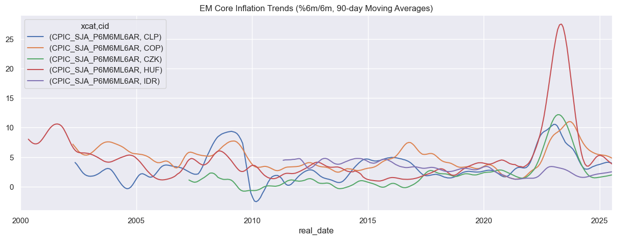
Applying window operations #
Often, rolling or expanding statistics are used to summarise time series’. These can be used to smooth local flunctuations.
Rolling statistics are calculated based on the most recent (specified) time units.
# Get core inflation statistics from 5 emerging markets
xcatx = ["CPIC_SJA_P6M6ML6AR"]
cidx = cids_em[:5]

dfx = df[df["xcat"].isin(xcatx) & df["cid"].isin(cidx)]

# Calculate 90 day rolling average for each selected emerging market core CPI
dfx_pivot = dfx.pivot(index = ["cid", "real_date"], columns="xcat", values="value").sort_index()
dfx_pivot_90rm = dfx_pivot.groupby(level=0).rolling(90, min_periods = 90).mean().reset_index(level=0,drop=True)

# Plot
dfx_pivot_90rm.unstack(0).plot(
    figsize=(15, 5),
    title="EM Core Inflation Trends (%6m/6m, 90-day Moving Averages)"
)
plt.show()
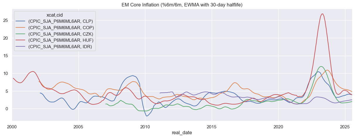
Expanding statistics compute values over the full available history up to each point, capturing evolving long-term trends. This is often combined with exponential weighting to emphasize recent observations.
# Exponentially weighted moving average of inflation
dfx_pivot = dfx.pivot(index=["cid", "real_date"], columns="xcat", values="value").sort_index()

# Compute EWMA with halflife = 30 days
dfx_pivot_ewm = (dfx_pivot.groupby(level=0).apply(lambda x: x.ewm(halflife=30, min_periods=30).mean()).reset_index(level=0, drop=True))

# Plot
dfx_pivot_ewm.unstack(0).plot(
    figsize=(15, 5),
    title="EM Core Inflation (%6m/6m, EWMA with 30-day halflife)"
)
plt.show()