Boosting macro trading signals #
Get packages and JPMaQS data #
import numpy as np
import pandas as pd
from pandas import Timestamp
import matplotlib.pyplot as plt
from datetime import date
import seaborn as sns
import os

from datetime import datetime

import macrosynergy.management as msm
import macrosynergy.panel as msp
import macrosynergy.signal as mss
import macrosynergy.pnl as msn
import macrosynergy.visuals as msv
import macrosynergy.learning as msl
from macrosynergy.management.utils import merge_categories

from sklearn.linear_model import LinearRegression, Ridge
from sklearn.ensemble import RandomForestRegressor, AdaBoostRegressor
from sklearn.metrics import make_scorer, r2_score

from macrosynergy.download import JPMaQSDownload

pd.set_option("display.width", 400)
import warnings

warnings.simplefilter("ignore")

np.random.seed(42)
RANDOM_STATE = np.random.randint(low=1, high=100)
# Cross-sections of interest

cids_dm = [
    "AUD",
    "CAD",
    "CHF",
    "EUR",
    "GBP",
    "JPY",
    "NOK",
    "NZD",
    "SEK",
    "USD",
]  # DM currency areas
cids_latm = ["BRL", "COP", "CLP", "MXN", "PEN"]  # Latam countries
cids_emea = ["CZK", "HUF", "ILS", "PLN", "RON", "RUB", "TRY", "ZAR"]  # EMEA countries
cids_emas = [
    "CNY",
    "IDR",
    "INR",
    "KRW",
    "MYR",
    "PHP",
    "SGD",
    "THB",
    "TWD",
]  # EM Asia countries

cids_dmfx = sorted(list(set(cids_dm) - set(["USD"])))
cids_emfx = sorted(set(cids_latm + cids_emea + cids_emas) - set(["CNY", "SGD"]))

cids_fx = sorted(cids_dmfx + cids_emfx)
cids = sorted(cids_dm + cids_emfx)

cids_eur = ["CHF", "NOK", "SEK", "PLN", "HUF", "CZK", "RON"]  # trading against EUR
cids_eud = ["GBP", "RUB", "TRY"]  # trading against EUR and USD
cids_usd = list(set(cids_fx) - set(cids_eur + cids_eud))  # trading against USD
# Quantamental categories

# Economic activity

output_growth = [
    "INTRGDP_NSA_P1M1ML12_3MMA",
    "RGDPTECH_SA_P1M1ML12_3MMA",
    "IP_SA_P6M6ML6AR",
    "IP_SA_P1M1ML12_3MMA",
]
mbconf_change = [
    "MBCSCORE_SA_D3M3ML3",
    "MBCSCORE_SA_D6M6ML6",
    "MBCSCORE_SA_D1Q1QL1",
    "MBCSCORE_SA_D2Q2QL2",
]
labtight_change = [
    "EMPL_NSA_P1M1ML12_3MMA",
    "EMPL_NSA_P1Q1QL4",
    "UNEMPLRATE_NSA_3MMA_D1M1ML12",
    "UNEMPLRATE_NSA_D1Q1QL4",
    "UNEMPLRATE_SA_D6M6ML6",
    "UNEMPLRATE_SA_D2Q2QL2",
]
cons_growth = [
    "RPCONS_SA_P1M1ML12_3MMA",
    "RPCONS_SA_P1Q1QL4",
    "CCSCORE_SA",
    "CCSCORE_SA_D6M6ML6",
    "CCSCORE_SA_D2Q2QL2",
    "RRSALES_SA_P1M1ML12_3MMA",
    "RRSALES_SA_P1Q1QL4",
]

# Monetary policy

cpi_inf = [
    "CPIH_SA_P1M1ML12",
    "CPIH_SJA_P6M6ML6AR",
    "CPIC_SA_P1M1ML12",
    "CPIC_SJA_P6M6ML6AR",
    "INFE2Y_JA",
]
pcredit_growth = ["PCREDITBN_SJA_P1M1ML12", "PCREDITGDP_SJA_D1M1ML12"]
real_rates = ["RIR_NSA", "RYLDIRS05Y_NSA", "FXCRR_NSA", "FXCRR_VT10", "FXCRRHvGDRB_NSA"]
liq_expansion = [
    "MBASEGDP_SA_D1M1ML3",
    "MBASEGDP_SA_D1M1ML6",
    "INTLIQGDP_NSA_D1M1ML3",
    "INTLIQGDP_NSA_D1M1ML6",
]

# External position and valuation

xbal_ratch = [
    "CABGDPRATIO_NSA_12MMA",
    "BXBGDPRATIO_NSA_12MMA",
    "MTBGDPRATIO_SA_6MMA_D1M1ML6",
    "BXBGDPRATIO_NSA_12MMA_D1M1ML3",
]
iliabs_accum = [
    "IIPLIABGDP_NSA_D1Mv2YMA",
    "IIPLIABGDP_NSA_D1Mv5YMA",
]
ppp_overval = [
    "PPPFXOVERVALUE_NSA_P1DvLTXL1",
    "PPPFXOVERVALUE_NSA_D1M60ML1",
]
reer_apprec = [
    "REER_NSA_P1M60ML1",
]

# Price competitiveness and dynamics

tot_pchange = [
    "CTOT_NSA_P1W4WL1",
    "CTOT_NSA_P1M1ML12",
    "CTOT_NSA_P1M60ML1",
    "MTOT_NSA_P1M60ML1",
]
ppi_pchange = [
    "PGDPTECH_SA_P1M1ML12_3MMA",
    "PGDPTECHX_SA_P1M1ML12_3MMA",
    "PPIH_NSA_P1M1ML12",
    "PPIH_SA_P6M6ML6AR",
]
# Complementary categories

complements = ["WFORCE_NSA_P1Y1YL1_5YMM", "INFTEFF_NSA", "RGDP_SA_P1Q1QL4_20QMM"]

# ALl macro categories

econ_act = output_growth + mbconf_change + labtight_change + cons_growth
mon_pol = cpi_inf + pcredit_growth + real_rates + liq_expansion
ext_pos = xbal_ratch + iliabs_accum + ppp_overval + reer_apprec
price_dyn = tot_pchange + ppi_pchange

macro = econ_act + mon_pol + ext_pos + price_dyn + complements

# Market categories

blacks = [
    "FXTARGETED_NSA",
    "FXUNTRADABLE_NSA",
]
rets = [
    "FXXR_NSA",
    "FXXR_VT10",
    "FXXRHvGDRB_NSA",
]

mkts = blacks + rets

# ALl categories

xcats = macro + mkts

# Tickers for download

single_tix = ["USD_GB10YXR_NSA", "EUR_FXXR_NSA", "USD_EQXR_NSA"]
tickers = [cid + "_" + xcat for cid in cids for xcat in xcats] + single_tix
# Download series from J.P. Morgan DataQuery by tickers

start_date = "1990-01-01"
end_date = (pd.Timestamp.today() - pd.offsets.BDay(1)).strftime("%Y-%m-%d")

# Retrieve credentials

oauth_id = os.getenv("DQ_CLIENT_ID")  # Replace with own client ID
oauth_secret = os.getenv("DQ_CLIENT_SECRET")  # Replace with own secret

# Download from DataQuery

downloader = JPMaQSDownload(client_id=oauth_id, client_secret=oauth_secret)
df = downloader.download(
    tickers=tickers,
    start_date=start_date,
    end_date=end_date,
    metrics=["value"],
    suppress_warning=True,
    show_progress=True,
)

dfx = df.copy()
dfx.info()
Downloading data from JPMaQS.
Timestamp UTC:  2025-08-13 11:13:47
Connection successful!
Requesting data: 100%|█████████████████████████████████████████████████████████████████| 94/94 [00:20<00:00,  4.52it/s]
Downloading data: 100%|████████████████████████████████████████████████████████████████| 94/94 [01:04<00:00,  1.45it/s]
Some expressions are missing from the downloaded data. Check logger output for complete list.
273 out of 1862 expressions are missing. To download the catalogue of all available expressions and filter the unavailable expressions, set `get_catalogue=True` in the call to `JPMaQSDownload.download()`.
<class 'pandas.core.frame.DataFrame'>
RangeIndex: 11335886 entries, 0 to 11335885
Data columns (total 4 columns):
 #   Column     Dtype
---  ------     -----
 0   real_date  datetime64[ns]
 1   cid        object
 2   xcat       object
 3   value      float64
dtypes: datetime64[ns](1), float64(1), object(2)
memory usage: 345.9+ MB
Renaming, availability and blacklisting #
Renaming quarterly categories #
dict_repl = {
    "EMPL_NSA_P1Q1QL4": "EMPL_NSA_P1M1ML12_3MMA",
    "UNEMPLRATE_NSA_D1Q1QL4": "UNEMPLRATE_NSA_3MMA_D1M1ML12",
    "UNEMPLRATE_SA_D2Q2QL2": "UNEMPLRATE_SA_D6M6ML6",
    "MBCSCORE_SA_D1Q1QL1": "MBCSCORE_SA_D3M3ML3",
    "MBCSCORE_SA_D2Q2QL2": "MBCSCORE_SA_D6M6ML6",
    "RPCONS_SA_P1Q1QL4": "RPCONS_SA_P1M1ML12_3MMA",
    "CCSCORE_SA_D2Q2QL2": "CCSCORE_SA_D6M6ML6",
    "RRSALES_SA_P1Q1QL4": "RRSALES_SA_P1M1ML12_3MMA",
}

for key, value in dict_repl.items():
    dfx["xcat"] = dfx["xcat"].str.replace(key, value)
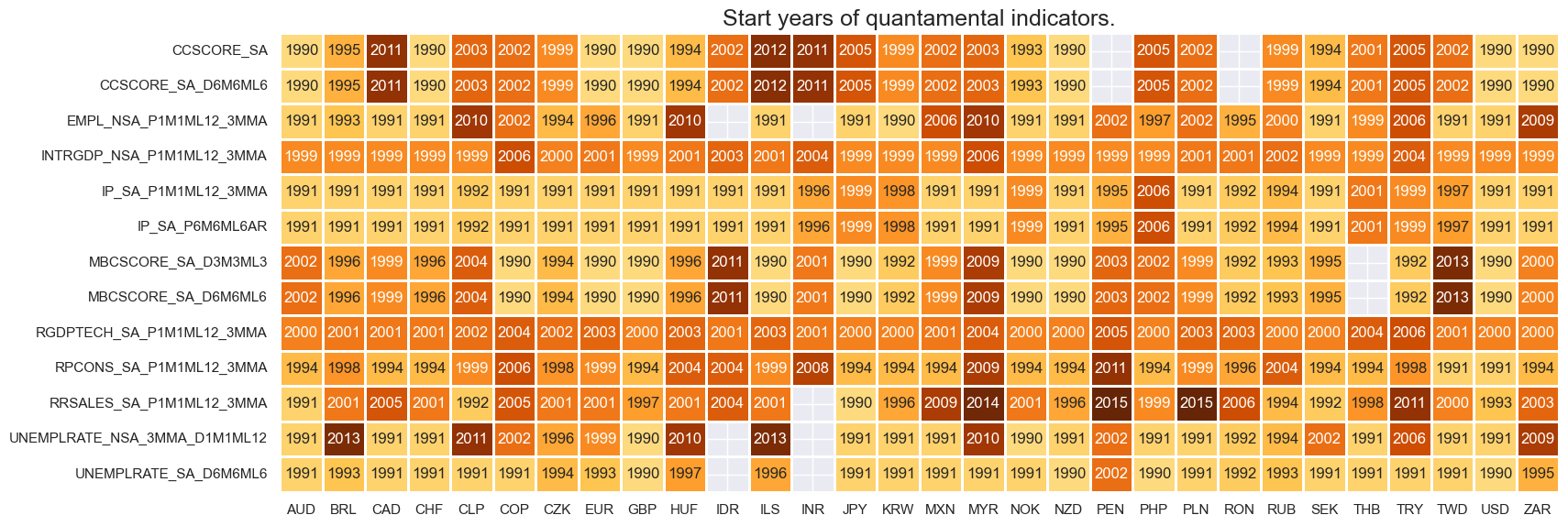
Check availability #
xcatx = econ_act
msm.check_availability(df=dfx, xcats=xcatx, cids=cids, missing_recent=False)
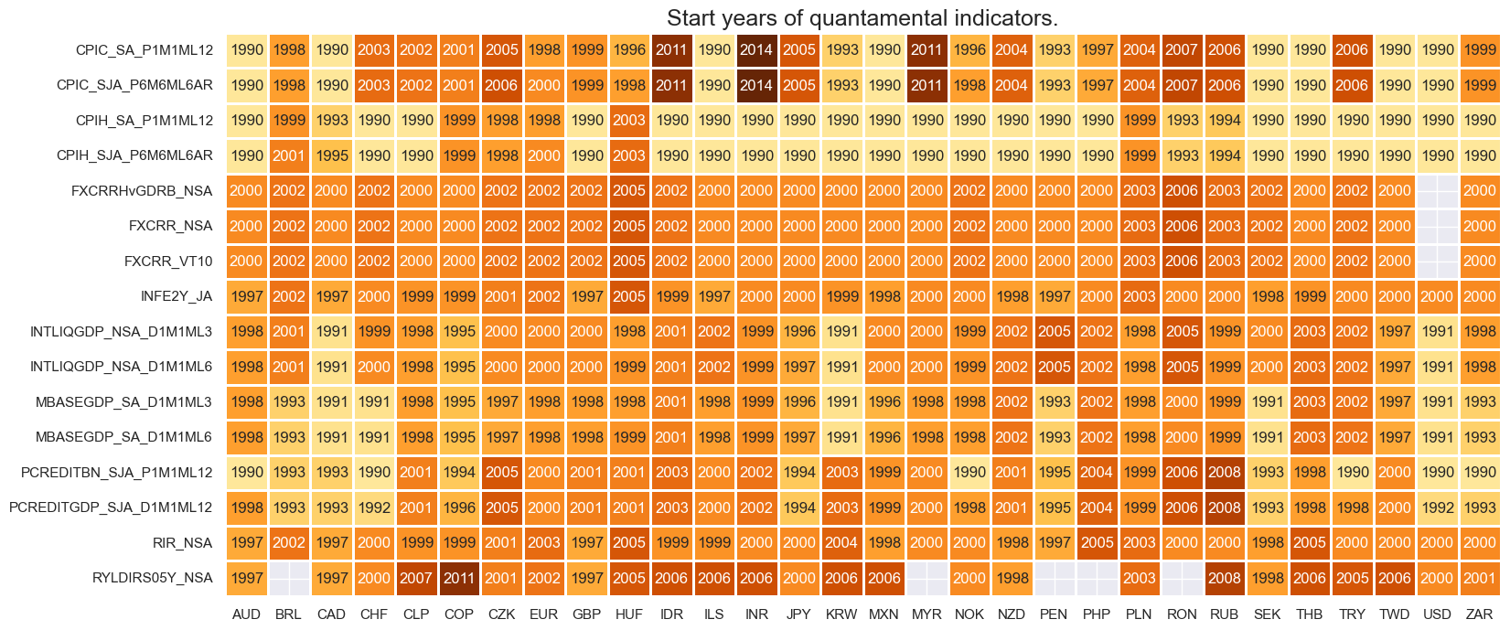
xcatx = mon_pol
msm.check_availability(df=dfx, xcats=xcatx, cids=cids, missing_recent=False)
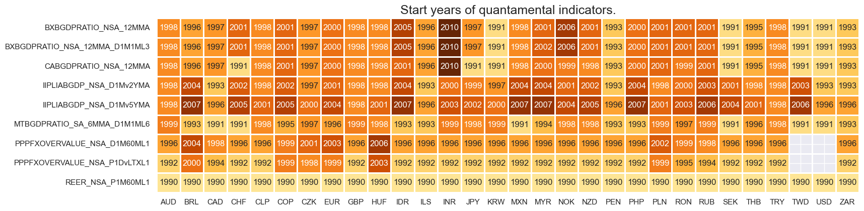
xcatx = ext_pos
msm.check_availability(df=dfx, xcats=xcatx, cids=cids, missing_recent=False)
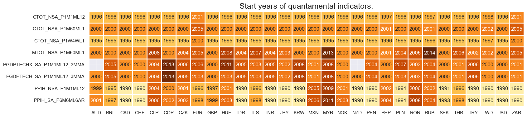
xcatx = price_dyn
msm.check_availability(df=dfx, xcats=xcatx, cids=cids, missing_recent=False)
Blacklisting dictionary for empirical research #
# Create blacklisting dictionary

dfb = df[df["xcat"].isin(["FXTARGETED_NSA", "FXUNTRADABLE_NSA"])].loc[
    :, ["cid", "xcat", "real_date", "value"]
]
dfba = (
    dfb.groupby(["cid", "real_date"])
    .aggregate(value=pd.NamedAgg(column="value", aggfunc="max"))
    .reset_index()
)
dfba["xcat"] = "FXBLACK"
fxblack = msp.make_blacklist(dfba, "FXBLACK")
fxblack
{'BRL': (Timestamp('2012-12-03 00:00:00'), Timestamp('2013-09-30 00:00:00')),
 'CHF': (Timestamp('2011-10-03 00:00:00'), Timestamp('2015-01-30 00:00:00')),
 'CZK': (Timestamp('2014-01-01 00:00:00'), Timestamp('2017-07-31 00:00:00')),
 'ILS': (Timestamp('1999-01-01 00:00:00'), Timestamp('2005-12-30 00:00:00')),
 'INR': (Timestamp('1999-01-01 00:00:00'), Timestamp('2004-12-31 00:00:00')),
 'MYR_1': (Timestamp('1999-01-01 00:00:00'), Timestamp('2007-11-30 00:00:00')),
 'MYR_2': (Timestamp('2018-07-02 00:00:00'), Timestamp('2025-08-12 00:00:00')),
 'PEN': (Timestamp('2021-07-01 00:00:00'), Timestamp('2021-07-30 00:00:00')),
 'RON': (Timestamp('1999-01-01 00:00:00'), Timestamp('2005-11-30 00:00:00')),
 'RUB_1': (Timestamp('1999-01-01 00:00:00'), Timestamp('2005-11-30 00:00:00')),
 'RUB_2': (Timestamp('2022-02-01 00:00:00'), Timestamp('2025-08-12 00:00:00')),
 'THB': (Timestamp('2007-01-01 00:00:00'), Timestamp('2008-11-28 00:00:00')),
 'TRY_1': (Timestamp('1999-01-01 00:00:00'), Timestamp('2003-09-30 00:00:00')),
 'TRY_2': (Timestamp('2020-01-01 00:00:00'), Timestamp('2024-07-31 00:00:00'))}
Factor construction and checks #
# Initiate category dictionary for thematic factors

dict_themes = {}

# Initiate labeling dictionary

dict_lab = {}
Economic activity factors #
# Governing dictionary for constituent factors

dict_ea = {
    "OUTPUT_GROWTH": {
        "INTRGDP_NSA_P1M1ML12_3MMA": ["vBM", ""],
        "RGDPTECH_SA_P1M1ML12_3MMA": ["vBM", ""],
        "IP_SA_P6M6ML6AR": ["vBM", ""],
        "IP_SA_P1M1ML12_3MMA": ["vBM", ""],
    },
    "MBC_CHANGE": {
        "MBCSCORE_SA_D3M3ML3": ["", ""],
        "MBCSCORE_SA_D6M6ML6": ["", ""],
    },
    "LAB_TIGHT": {
        "EMPL_NSA_P1M1ML12_3MMA": ["vBM", ""],
        "UNEMPLRATE_NSA_3MMA_D1M1ML12": ["vBM", "_NEG"],
        "UNEMPLRATE_SA_D6M6ML6": ["vBM", "_NEG"],
    },
    "CONS_GROWTH": {
        "RPCONS_SA_P1M1ML12_3MMA": ["vBM", ""],
        "CCSCORE_SA": ["vBM", ""],
        "CCSCORE_SA_D6M6ML6": ["vBM", ""],
        "RRSALES_SA_P1M1ML12_3MMA": ["vBM", ""],
    },
}

# Dictionary for transformed category names

dicx_ea = {}
# Add labels (in final transformed form)
dict_lab["OUTPUT_GROWTHZN"] = "Relative output growth"
dict_lab["MBC_CHANGEZN"] = "Industry confidence change"
dict_lab["LAB_TIGHTZN"] = "Relative labor tightening"
dict_lab["CONS_GROWTHZN"] = "Relative consumption growth"
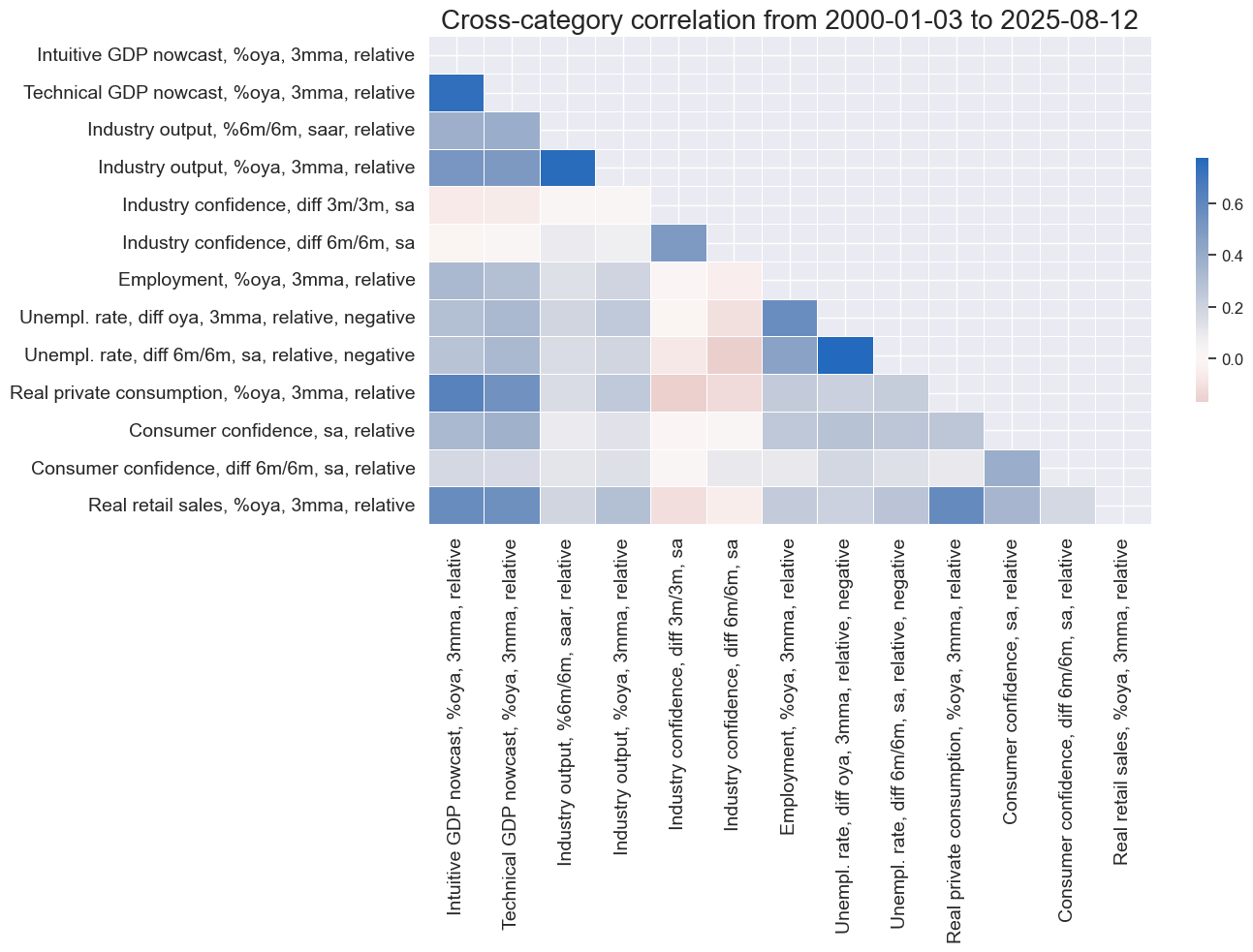
dict_lab["INTRGDP_NSA_P1M1ML12_3MMAvBMZN"] = (
"Intuitive GDP nowcast, %oya, 3mma, relative"
)
dict_lab["RGDPTECH_SA_P1M1ML12_3MMAvBMZN"] = (
"Technical GDP nowcast, %oya, 3mma, relative"
)
dict_lab["IP_SA_P6M6ML6ARvBMZN"] = "Industry output, %6m/6m, saar, relative"
dict_lab["IP_SA_P1M1ML12_3MMAvBMZN"] = "Industry output, %oya, 3mma, relative"
dict_lab["MBCSCORE_SA_D3M3ML3ZN"] = "Industry confidence, diff 3m/3m, sa"
dict_lab["MBCSCORE_SA_D6M6ML6ZN"] = "Industry confidence, diff 6m/6m, sa"
dict_lab["EMPL_NSA_P1M1ML12_3MMAvBMZN"] = "Employment, %oya, 3mma, relative"
dict_lab["UNEMPLRATE_NSA_3MMA_D1M1ML12vBM_NEGZN"] = (
"Unempl. rate, diff oya, 3mma, relative, negative"
)
dict_lab["UNEMPLRATE_SA_D6M6ML6vBM_NEGZN"] = (
"Unempl. rate, diff 6m/6m, sa, relative, negative"
)
dict_lab["RPCONS_SA_P1M1ML12_3MMAvBMZN"] = (
"Real private consumption, %oya, 3mma, relative"
)
dict_lab["CCSCORE_SAvBMZN"] = "Consumer confidence, sa, relative"
dict_lab["CCSCORE_SA_D6M6ML6vBMZN"] = "Consumer confidence, diff 6m/6m, sa, relative"
dict_lab["RRSALES_SA_P1M1ML12_3MMAvBMZN"] = "Real retail sales, %oya, 3mma, relative"
# Production of factors and thematic factors

dix = dict_ea
dicx = dicx_ea

for fact in dix.keys():

    # Original factors

    xcatx = list(dix[fact].keys())
    dicx[fact] = {}
    dicx[fact]["OR"] = xcatx

    # Relatives to benchmark (if required)

    vbms = [values[0] for values in dix[fact].values()]
    xcatxx = [xc for xc, bm in zip(xcatx, vbms) if bm == "vBM"]

    if len(xcatxx) > 0:
        dfa_usd = msp.make_relative_value(
            dfx, xcatxx, cids_usd, basket=["USD"], postfix="vBM"
        )
        dfa_eur = msp.make_relative_value(
            dfx, xcatxx, cids_eur, basket=["EUR"], postfix="vBM"
        )
        dfa_eud = msp.make_relative_value(
            dfx, xcatxx, cids_eud, basket=["EUR", "USD"], postfix="vBM"
        )
        dfa = pd.concat([dfa_eur, dfa_usd, dfa_eud])
        dfx = msm.update_df(dfx, dfa)

    dicx[fact]["BM"] = [xc + bm for xc, bm in zip(xcatx, vbms)]

    # Sign for hypothesized positive relation

    xcatxx = dicx[fact]["BM"]
    negs = [values[1] for values in dix[fact].values()]
    calcs = []

    for xc, neg in zip(xcatxx, negs):
        if neg == "_NEG":
            calcs += [f"{xc}_NEG = - {xc}"]

    if len(calcs) > 0:
        dfa = msp.panel_calculator(dfx, calcs=calcs, cids=cids_fx)
        dfx = msm.update_df(dfx, dfa)

    dicx[fact]["SG"] = [xc + neg for xc, neg in zip(xcatxx, negs)]

    # Sequential scoring

    xcatxx = dicx[fact]["SG"]
    cidx = cids_fx
    dfa = pd.DataFrame(columns=list(dfx.columns))

    for xc in xcatxx:
        dfaa = msp.make_zn_scores(
            dfx,
            xcat=xc,
            cids=cidx,
            sequential=True,
            min_obs=261 * 3,
            neutral="zero",
            pan_weight=1,
            thresh=3,
            postfix="ZN",
            est_freq="m",
        )
        dfa = msm.update_df(dfa, dfaa)

    dfx = msm.update_df(dfx, dfa)
    dicx[fact]["ZN"] = [xc + "ZN" for xc in xcatxx]
# Correlation matrix of final constituents

xcatx = [item for value in dicx_ea.values() if "ZN" in value for item in value["ZN"]]
cidx = cids_fx
sdate = "2000-01-01"
labels = [dict_lab[xc] for xc in xcatx]


msp.correl_matrix(
    dfx,
    xcats=xcatx,
    cids=cidx,
    start=sdate,
    freq="M",
    cluster=False,
    title=None,
    size=(14, 10),
    xcat_labels=labels,
)
# Factors and re-scoring
dicx = dicx_ea
cidx = cids_fx

factors = list(dicx.keys())

# Factors as average of constituent scores

for fact in factors:
    xcatx = dicx[fact]["ZN"]

    dfa = msp.linear_composite(
        dfx,
        xcats=xcatx,
        cids=cidx,
        complete_xcats=False,
        new_xcat=fact,
    )
    dfx = msm.update_df(dfx, dfa)

# Sequential re-scoring

dfa = pd.DataFrame(columns=list(dfx.columns))

for fact in factors:
    dfaa = msp.make_zn_scores(
        dfx,
        xcat=fact,
        cids=cidx,
        sequential=True,
        min_obs=261 * 3,
        neutral="zero",
        pan_weight=1,
        thresh=3,
        postfix="ZN",
        est_freq="m",
    )
    dfa = msm.update_df(dfa, dfaa)

dfx = msm.update_df(dfx, dfa)

dict_themes["REL_ECON_GROWTH"] = [fact + "ZN" for fact in factors]
Monetary policy factors #
# Preparation of categories for constituent factors

cidx = cids

# Preparation: for relative target deviations, we need denominator bases that should never be less than 2

dfa = msp.panel_calculator(df, ["INFTEBASIS = INFTEFF_NSA.clip(lower=2)"], cids=cidx)
dfx = msm.update_df(dfx, dfa)

xcatx = cpi_inf + pcredit_growth


calcs = [f"XR{xc} = ( {xc} - INFTEFF_NSA ) / INFTEBASIS" for xc in xcatx]
dfa = msp.panel_calculator(dfx, calcs=calcs, cids=cidx)
dfx = msm.update_df(dfx, dfa)
# Governing dictionary for constituent factors

dict_mp = {
    "EXCESS_INFLATION": {
        "XRCPIH_SA_P1M1ML12": ["vBM", ""],
        "XRCPIH_SJA_P6M6ML6AR": ["vBM", ""],
        "XRCPIC_SA_P1M1ML12": ["vBM", ""],
        "XRCPIC_SJA_P6M6ML6AR": ["vBM", ""],
        "XRINFE2Y_JA": ["vBM", ""],
    },
    "XPCREDIT_GROWTH": {
        "XRPCREDITBN_SJA_P1M1ML12": ["vBM", ""],
        "XRPCREDITGDP_SJA_D1M1ML12": ["vBM", ""],
    },
    "REAL_RATES": {
        "RIR_NSA": ["vBM", ""],
        "RYLDIRS05Y_NSA": ["vBM", ""],
        "FXCRR_NSA": ["", ""],
        "FXCRR_VT10": ["", ""],
        "FXCRRHvGDRB_NSA": ["", ""],
    },
    "LIQ_TIGHT": {
        "MBASEGDP_SA_D1M1ML3": ["vBM", "_NEG"],
        "MBASEGDP_SA_D1M1ML6": ["vBM", "_NEG"],
        "INTLIQGDP_NSA_D1M1ML3": ["vBM", "_NEG"],
        "INTLIQGDP_NSA_D1M1ML6": ["vBM", "_NEG"],
    },
}

# Dictionary for transformed category names

dicx_mp = {}
# Add labels (in final transformed form)
dict_lab["EXCESS_INFLATIONZN"] = "Relative excess inflation ratios"
dict_lab["XPCREDIT_GROWTHZN"] = "Relative excess credit growth"
dict_lab["REAL_RATESZN"] = "Real rate differentials and carry"
dict_lab["LIQ_TIGHTZN"] = "Relative liquidity tightening"
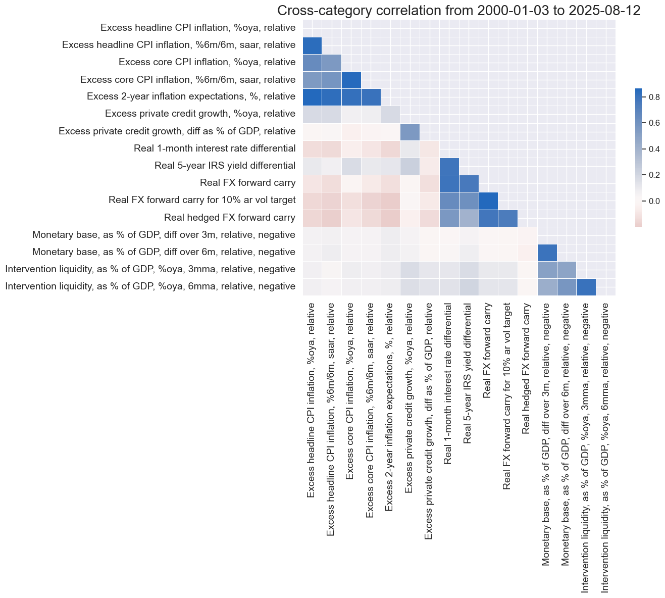
dict_lab["XRCPIH_SA_P1M1ML12vBMZN"] = "Excess headline CPI inflation, %oya, relative"
dict_lab["XRCPIH_SJA_P6M6ML6ARvBMZN"] = (
"Excess headline CPI inflation, %6m/6m, saar, relative"
)
dict_lab["XRCPIC_SA_P1M1ML12vBMZN"] = "Excess core CPI inflation, %oya, relative"
dict_lab["XRCPIC_SJA_P6M6ML6ARvBMZN"] = (
"Excess core CPI inflation, %6m/6m, saar, relative"
)
dict_lab["XRINFE2Y_JAvBMZN"] = "Excess 2-year inflation expectations, %, relative"
dict_lab["XRPCREDITBN_SJA_P1M1ML12vBMZN"] = (
"Excess private credit growth, %oya, relative"
)
dict_lab["XRPCREDITGDP_SJA_D1M1ML12vBMZN"] = (
"Excess private credit growth, diff as % of GDP, relative"
)
dict_lab["RIR_NSAvBMZN"] = "Real 1-month interest rate differential"
dict_lab["RYLDIRS05Y_NSAvBMZN"] = "Real 5-year IRS yield differential"
dict_lab["FXCRR_NSAZN"] = "Real FX forward carry"
dict_lab["FXCRR_VT10ZN"] = "Real FX forward carry for 10% ar vol target"
dict_lab["FXCRRHvGDRB_NSAZN"] = "Real hedged FX forward carry"
dict_lab["MBASEGDP_SA_D1M1ML3vBM_NEGZN"] = (
"Monetary base, as % of GDP, diff over 3m, relative, negative"
)
dict_lab["MBASEGDP_SA_D1M1ML6vBM_NEGZN"] = (
"Monetary base, as % of GDP, diff over 6m, relative, negative"
)
dict_lab["INTLIQGDP_NSA_D1M1ML3vBM_NEGZN"] = (
"Intervention liquidity, as % of GDP, %oya, 3mma, relative, negative"
)
dict_lab["INTLIQGDP_NSA_D1M1ML6vBM_NEGZN"] = (
"Intervention liquidity, as % of GDP, %oya, 6mma, relative, negative"
)
# Production of factors and thematic factors

dix = dict_mp
dicx = dicx_mp

for fact in dix.keys():

    # Original factors

    xcatx = list(dix[fact].keys())
    dicx[fact] = {}
    dicx[fact]["OR"] = xcatx

    # Relatives to benchmark (if required)

    vbms = [values[0] for values in dix[fact].values()]
    xcatxx = [xc for xc, bm in zip(xcatx, vbms) if bm == "vBM"]

    if len(xcatxx) > 0:
        dfa_usd = msp.make_relative_value(
            dfx, xcatxx, cids_usd, basket=["USD"], postfix="vBM"
        )
        dfa_eur = msp.make_relative_value(
            dfx, xcatxx, cids_eur, basket=["EUR"], postfix="vBM"
        )
        dfa_eud = msp.make_relative_value(
            dfx, xcatxx, cids_eud, basket=["EUR", "USD"], postfix="vBM"
        )
        dfa = pd.concat([dfa_eur, dfa_usd, dfa_eud])
        dfx = msm.update_df(dfx, dfa)

    dicx[fact]["BM"] = [xc + bm for xc, bm in zip(xcatx, vbms)]

    # Sign for hypothesized positive relation

    xcatxx = dicx[fact]["BM"]
    negs = [values[1] for values in dix[fact].values()]
    calcs = []

    for xc, neg in zip(xcatxx, negs):
        if neg == "_NEG":
            calcs += [f"{xc}_NEG = - {xc}"]

    if len(calcs) > 0:
        dfa = msp.panel_calculator(dfx, calcs=calcs, cids=cids_fx)
        dfx = msm.update_df(dfx, dfa)

    dicx[fact]["SG"] = [xc + neg for xc, neg in zip(xcatxx, negs)]

    # Sequential scoring

    xcatxx = dicx[fact]["SG"]
    cidx = cids_fx
    dfa = pd.DataFrame(columns=list(dfx.columns))

    for xc in xcatxx:
        dfaa = msp.make_zn_scores(
            dfx,
            xcat=xc,
            cids=cidx,
            sequential=True,
            min_obs=261 * 3,
            neutral="zero",
            pan_weight=1,
            thresh=3,
            postfix="ZN",
            est_freq="m",
        )
        dfa = msm.update_df(dfa, dfaa)

    dfx = msm.update_df(dfx, dfa)
    dicx[fact]["ZN"] = [xc + "ZN" for xc in xcatxx]
# Correlation matrix of final constituents

xcatx = [item for value in dicx_mp.values() if "ZN" in value for item in value["ZN"]]
cidx = cids_fx
sdate = "2000-01-01"
labels = [dict_lab[xc] for xc in xcatx]


msp.correl_matrix(
    dfx,
    xcats=xcatx,
    cids=cidx,
    start=sdate,
    freq="M",
    cluster=False,
    title=None,
    size=(14, 12),
    xcat_labels=labels,
)
# Factors and re-scoring
dicx = dicx_mp
cidx = cids_fx

factors = list(dicx.keys())

# Factors as average of constituent scores

for fact in factors:
    xcatx = dicx[fact]["ZN"]

    dfa = msp.linear_composite(
        dfx,
        xcats=xcatx,
        cids=cidx,
        complete_xcats=False,
        new_xcat=fact,
    )
    dfx = msm.update_df(dfx, dfa)

# Sequential re-scoring

dfa = pd.DataFrame(columns=list(dfx.columns))

for fact in factors:
    dfaa = msp.make_zn_scores(
        dfx,
        xcat=fact,
        cids=cidx,
        sequential=True,
        min_obs=261 * 3,
        neutral="zero",
        pan_weight=1,
        thresh=3,
        postfix="ZN",
        est_freq="m",
    )
    dfa = msm.update_df(dfa, dfaa)

dfx = msm.update_df(dfx, dfa)

dict_themes["REL_MONPOL_TIGHT"] = [fact + "ZN" for fact in factors]
External position and valuation factors #
# Governing dictionary for constituent factors

dict_xv = {
    "EXTERNAL_BALANCES": {
        "CABGDPRATIO_NSA_12MMA": ["", ""],
        "BXBGDPRATIO_NSA_12MMA": ["", ""],
        "MTBGDPRATIO_SA_6MMA_D1M1ML6": ["", ""],
        "BXBGDPRATIO_NSA_12MMA_D1M1ML3": ["", ""],
    },
    "LIABILITIES_GROWTH": {
        "IIPLIABGDP_NSA_D1Mv2YMA": ["", "_NEG"],
        "IIPLIABGDP_NSA_D1Mv5YMA": ["", "_NEG"],
    },
    "FX_OVERVAL": {
        "PPPFXOVERVALUE_NSA_P1DvLTXL1": ["", "_NEG"],
        "PPPFXOVERVALUE_NSA_D1M60ML1": ["", "_NEG"],
        "REER_NSA_P1M60ML1": ["", "_NEG"],
    },
}

# Dictionary for transformed category names

dicx_xv = {}
# Add labels (in final transformed form)
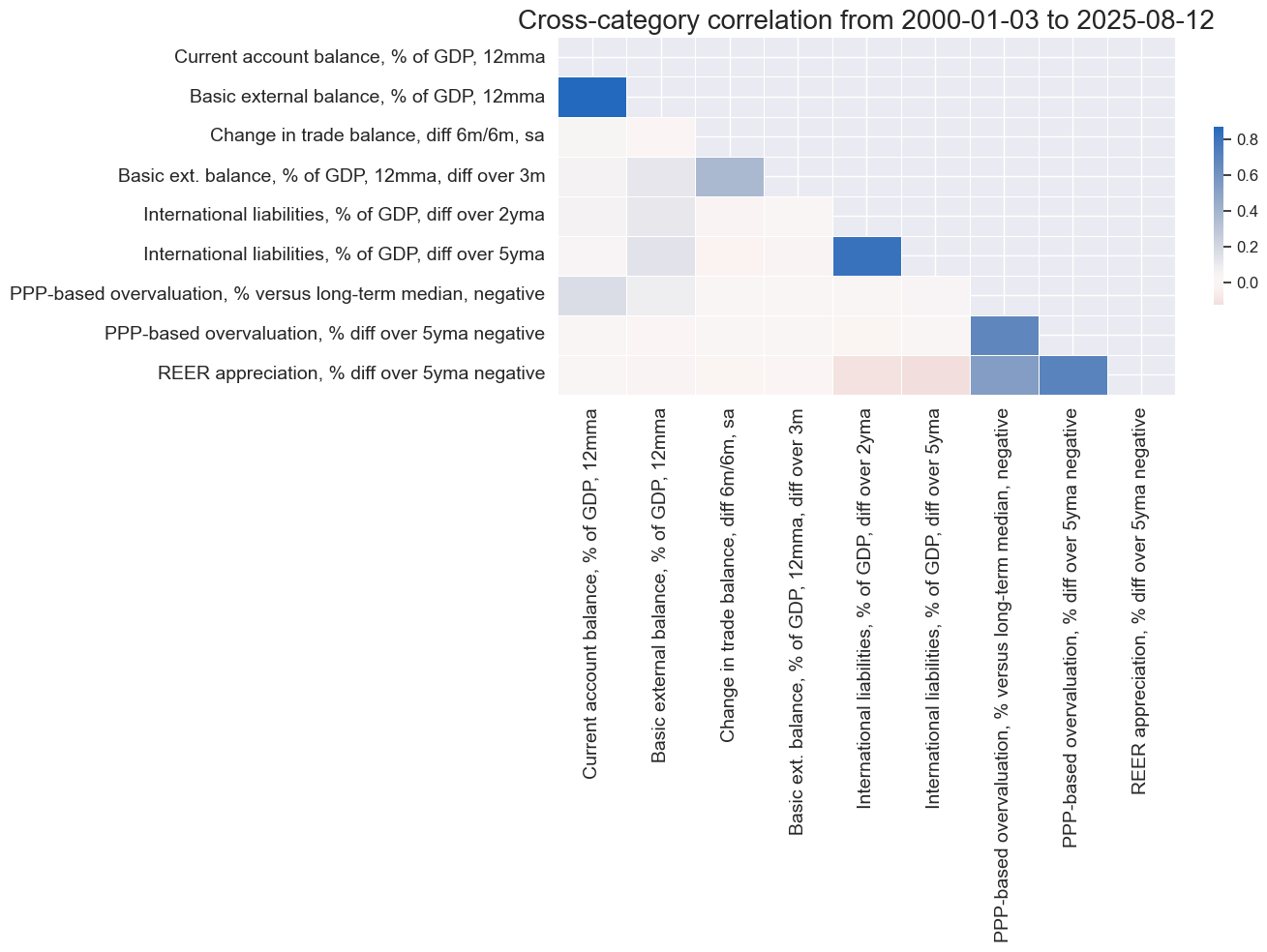
dict_lab["EXTERNAL_BALANCESZN"] = "External balances ratios"
dict_lab["LIABILITIES_GROWTHZN"] = "Liabilities growth (negative)"
dict_lab["FX_OVERVALZN"] = "FX overvaluation (negative)"
dict_lab["CABGDPRATIO_NSA_12MMAZN"] = "Current account balance, % of GDP, 12mma"
dict_lab["BXBGDPRATIO_NSA_12MMAZN"] = "Basic external balance, % of GDP, 12mma"
dict_lab["MTBGDPRATIO_SA_6MMA_D1M1ML6ZN"] = "Change in trade balance, diff 6m/6m, sa"
dict_lab["BXBGDPRATIO_NSA_12MMA_D1M1ML3ZN"] = (
"Basic ext. balance, % of GDP, 12mma, diff over 3m"
)
dict_lab["IIPLIABGDP_NSA_D1Mv2YMA_NEGZN"] = (
"International liabilities, % of GDP, diff over 2yma"
)
dict_lab["IIPLIABGDP_NSA_D1Mv5YMA_NEGZN"] = (
"International liabilities, % of GDP, diff over 5yma"
)
dict_lab["PPPFXOVERVALUE_NSA_P1DvLTXL1_NEGZN"] = (
"PPP-based overvaluation, % versus long-term median, negative"
)
dict_lab["PPPFXOVERVALUE_NSA_D1M60ML1_NEGZN"] = (
"PPP-based overvaluation, % diff over 5yma negative"
)
dict_lab["REER_NSA_P1M60ML1_NEGZN"] = "REER appreciation, % diff over 5yma negative"
# Production of factors and thematic factors

dix = dict_xv
dicx = dicx_xv

for fact in dix.keys():

    # Original factors

    xcatx = list(dix[fact].keys())
    dicx[fact] = {}
    dicx[fact]["OR"] = xcatx

    # Relatives to benchmark (if required)

    vbms = [values[0] for values in dix[fact].values()]
    xcatxx = [xc for xc, bm in zip(xcatx, vbms) if bm == "vBM"]

    if len(xcatxx) > 0:
        dfa_usd = msp.make_relative_value(
            dfx, xcatxx, cids_usd, basket=["USD"], postfix="vBM"
        )
        dfa_eur = msp.make_relative_value(
            dfx, xcatxx, cids_eur, basket=["EUR"], postfix="vBM"
        )
        dfa_eud = msp.make_relative_value(
            dfx, xcatxx, cids_eud, basket=["EUR", "USD"], postfix="vBM"
        )
        dfa = pd.concat([dfa_eur, dfa_usd, dfa_eud])
        dfx = msm.update_df(dfx, dfa)

    dicx[fact]["BM"] = [xc + bm for xc, bm in zip(xcatx, vbms)]

    # Sign for hypothesized positive relation

    xcatxx = dicx[fact]["BM"]
    negs = [values[1] for values in dix[fact].values()]
    calcs = []

    for xc, neg in zip(xcatxx, negs):
        if neg == "_NEG":
            calcs += [f"{xc}_NEG = - {xc}"]

    if len(calcs) > 0:
        dfa = msp.panel_calculator(dfx, calcs=calcs, cids=cids_fx)
        dfx = msm.update_df(dfx, dfa)

    dicx[fact]["SG"] = [xc + neg for xc, neg in zip(xcatxx, negs)]

    # Sequential scoring

    xcatxx = dicx[fact]["SG"]
    cidx = cids_fx
    dfa = pd.DataFrame(columns=list(dfx.columns))

    for xc in xcatxx:
        dfaa = msp.make_zn_scores(
            dfx,
            xcat=xc,
            cids=cidx,
            sequential=True,
            min_obs=261 * 3,
            neutral="zero",
            pan_weight=1,
            thresh=3,
            postfix="ZN",
            est_freq="m",
        )
        dfa = msm.update_df(dfa, dfaa)

    dfx = msm.update_df(dfx, dfa)
    dicx[fact]["ZN"] = [xc + "ZN" for xc in xcatxx]
# Correlation matrix of final constituents

xcatx = [item for value in dicx_xv.values() if "ZN" in value for item in value["ZN"]]
cidx = cids_fx
sdate = "2000-01-01"
labels = [dict_lab[xc] for xc in xcatx]

msp.correl_matrix(
    dfx,
    xcats=xcatx,
    cids=cidx,
    start=sdate,
    freq="M",
    cluster=False,
    title=None,
    size=(14, 10),
    xcat_labels=labels,
)
# Factors and re-scoring
dicx = dicx_xv
cidx = cids_fx

factors = list(dicx.keys())

# Factors as average of constituent scores

for fact in factors:
    xcatx = dicx[fact]["ZN"]

    dfa = msp.linear_composite(
        dfx,
        xcats=xcatx,
        cids=cidx,
        complete_xcats=False,
        new_xcat=fact,
    )
    dfx = msm.update_df(dfx, dfa)

# Sequential re-scoring

dfa = pd.DataFrame(columns=list(dfx.columns))

for fact in factors:
    dfaa = msp.make_zn_scores(
        dfx,
        xcat=fact,
        cids=cidx,
        sequential=True,
        min_obs=261 * 3,
        neutral="zero",
        pan_weight=1,
        thresh=3,
        postfix="ZN",
        est_freq="m",
    )
    dfa = msm.update_df(dfa, dfaa)

dfx = msm.update_df(dfx, dfa)

dict_themes["EXTERNAL_VALUE"] = [fact + "ZN" for fact in factors]
Price competitiveness factors #
# Preparation of categories for constituent factors

xcatx = ppi_pchange
cidx = cids

calcs = [f"XR{xc} = ( {xc} - INFTEFF_NSA ) / INFTEBASIS" for xc in xcatx]
dfa = msp.panel_calculator(dfx, calcs=calcs, cids=cidx)
dfx = msm.update_df(dfx, dfa)
# Governing dictionary for constituent factors

dict_pc = {
    "EXCESS_PPIGROWTH": {
        "XRPGDPTECH_SA_P1M1ML12_3MMA": ["vBM", ""],
        "XRPPIH_NSA_P1M1ML12": ["vBM", ""],
    },
    "TOT_CHANGE": {
        "CTOT_NSA_P1W4WL1": ["", ""],
        "CTOT_NSA_P1M1ML12": ["", ""],
        "CTOT_NSA_P1M60ML1": ["", ""],
        "MTOT_NSA_P1M60ML1": ["", ""],
    },
}

# Dictionary for transformed category names

dicx_pc = {}
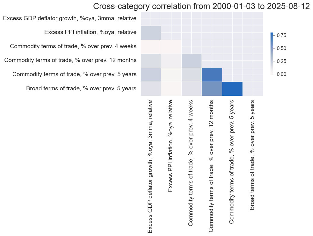
dict_lab["EXCESS_PPIGROWTHZN"] = "Relative excess producer price growth"
dict_lab["TOT_CHANGEZN"] = "Terms of change improvement"

dict_lab["XRPGDPTECH_SA_P1M1ML12_3MMAvBMZN"] = (
    "Excess GDP deflator growth, %oya, 3mma, relative"
)
dict_lab["XRPPIH_NSA_P1M1ML12vBMZN"] = "Excess PPI inflation, %oya, relative"

dict_lab["CTOT_NSA_P1W4WL1ZN"] = "Commodity terms of trade, % over prev. 4 weeks"
dict_lab["CTOT_NSA_P1M1ML12ZN"] = "Commodity terms of trade, % over prev. 12 months"
dict_lab["CTOT_NSA_P1M60ML1ZN"] = "Commodity terms of trade, % over prev. 5 years"
dict_lab["MTOT_NSA_P1M60ML1ZN"] = "Broad terms of trade, % over prev. 5 years"
# Production of factors and thematic factors

dix = dict_pc
dicx = dicx_pc

for fact in dix.keys():

    # Original factors

    xcatx = list(dix[fact].keys())
    dicx[fact] = {}
    dicx[fact]["OR"] = xcatx

    # Relatives to benchmark (if required)

    vbms = [values[0] for values in dix[fact].values()]
    xcatxx = [xc for xc, bm in zip(xcatx, vbms) if bm == "vBM"]

    if len(xcatxx) > 0:
        dfa_usd = msp.make_relative_value(
            dfx, xcatxx, cids_usd, basket=["USD"], postfix="vBM"
        )
        dfa_eur = msp.make_relative_value(
            dfx, xcatxx, cids_eur, basket=["EUR"], postfix="vBM"
        )
        dfa_eud = msp.make_relative_value(
            dfx, xcatxx, cids_eud, basket=["EUR", "USD"], postfix="vBM"
        )

        dfa = pd.concat([dfa_eur, dfa_usd, dfa_eud])
        dfx = msm.update_df(dfx, dfa)

    dicx[fact]["BM"] = [xc + bm for xc, bm in zip(xcatx, vbms)]

    # Sign for hypothesized positive relation

    xcatxx = dicx[fact]["BM"]
    negs = [values[1] for values in dix[fact].values()]
    calcs = []

    for xc, neg in zip(xcatxx, negs):
        if neg == "_NEG":
            calcs += [f"{xc}_NEG = - {xc}"]

    if len(calcs) > 0:
        dfa = msp.panel_calculator(dfx, calcs=calcs, cids=cids_fx)
        dfx = msm.update_df(dfx, dfa)

    dicx[fact]["SG"] = [xc + neg for xc, neg in zip(xcatxx, negs)]

    # Sequential scoring

    xcatxx = dicx[fact]["SG"]
    cidx = cids_fx
    dfa = pd.DataFrame(columns=list(dfx.columns))

    for xc in xcatxx:
        dfaa = msp.make_zn_scores(
            dfx,
            xcat=xc,
            cids=cidx,
            sequential=True,
            min_obs=261 * 3,
            neutral="zero",
            pan_weight=1,
            thresh=3,
            postfix="ZN",
            est_freq="m",
        )
        dfa = msm.update_df(dfa, dfaa)

    dfx = msm.update_df(dfx, dfa)
    dicx[fact]["ZN"] = [xc + "ZN" for xc in xcatxx]
# Correlation matrix of final constituents

xcatx = [item for value in dicx_pc.values() if "ZN" in value for item in value["ZN"]]
cidx = cids_fx
sdate = "2000-01-01"
labels = [dict_lab[xc] for xc in xcatx]


msp.correl_matrix(
    dfx,
    xcats=xcatx,
    cids=cidx,
    start=sdate,
    freq="M",
    cluster=False,
    title=None,
    size=(10, 8),
    xcat_labels=labels,
)
# Factors and re-scoring
dicx = dicx_pc
cidx = cids_fx

factors = list(dicx.keys())

# Factors as average of constituent scores

for fact in factors:
    xcatx = dicx[fact]["ZN"]

    dfa = msp.linear_composite(
        dfx,
        xcats=xcatx,
        cids=cidx,
        complete_xcats=False,
        new_xcat=fact,
    )
    dfx = msm.update_df(dfx, dfa)

# Sequential re-scoring

dfa = pd.DataFrame(columns=list(dfx.columns))

for fact in factors:
    dfaa = msp.make_zn_scores(
        dfx,
        xcat=fact,
        cids=cidx,
        sequential=True,
        min_obs=261 * 3,
        neutral="zero",
        pan_weight=1,
        thresh=3,
        postfix="ZN",
        est_freq="m",
    )
    dfa = msm.update_df(dfa, dfaa)

dfx = msm.update_df(dfx, dfa)

dict_themes["REL_PRICE_COMPETE"] = [fact + "ZN" for fact in factors]
Thematic factor calculation #
# Themes and re-scoring

cidx = cids_fx
themes = list(dict_themes.keys())

# Themes as average of factor scores

for theme in themes:
    xcatx = dict_themes[theme]

    dfa = msp.linear_composite(
        dfx,
        xcats=xcatx,
        cids=cidx,
        complete_xcats=False,
        new_xcat=theme,
    )
    dfx = msm.update_df(dfx, dfa)

# Sequential re-scoring

dfa = pd.DataFrame(columns=list(dfx.columns))

for theme in themes:
    dfaa = msp.make_zn_scores(
        dfx,
        xcat=theme,
        cids=cidx,
        sequential=True,
        min_obs=261 * 3,
        neutral="zero",
        pan_weight=1,
        thresh=3,
        postfix="ZN",
        est_freq="m",
    )
    dfa = msm.update_df(dfa, dfaa)

dfx = msm.update_df(dfx, dfa)

themez = [theme + "ZN" for theme in themes]
Signal optimization with machine learning #
General preparations #
# Candidate factors for optimization

fx_facts = list((*dicx_pc.keys(), *dicx_mp.keys(), *dicx_ea.keys(), *dicx_xv.keys()))
fx_factz = [f + "ZN" for f in fx_facts]
#fx_factz = themez

# Special labelling dictionary
dict_factz = {k: v for k, v in dict_lab.items() if k in fx_factz}
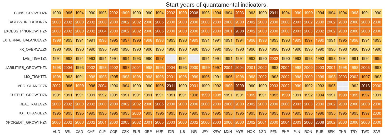
# Visualize availability of the factors
xcatx = fx_factz
msm.check_availability(df=dfx, xcats=xcatx, cids=cids, missing_recent=False)
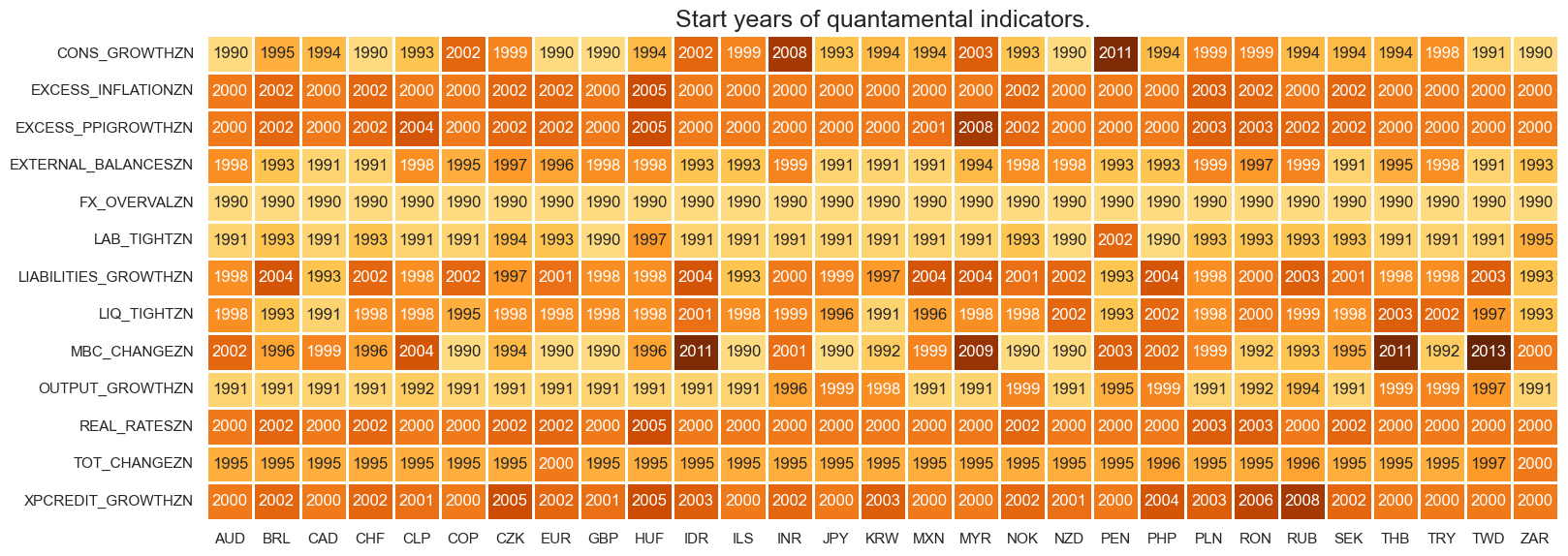
Imputation of factors #
Commenting out the below imputes Indonesian and Indian labour market tightness based on the average labour market tightness in Asia. Similarly for Thai manufacturing confidence.
dfa = msp.MeanPanelImputer(
    df = msm.reduce_df(df=dfx, xcats = ["LAB_TIGHTZN"], cids = cids_emas),
    xcats = ["LAB_TIGHTZN"],
    cids = ["IDR","INR"],
    min_cids = 5,
    postfix="",
).impute()

dfx = msm.update_df(dfx, dfa)
dfa = msp.MeanPanelImputer(
    df = msm.reduce_df(df=dfx, xcats = ["MBC_CHANGEZN"], cids = cids_emas),
    xcats = ["MBC_CHANGEZN"],
    cids = ["THB"],
    min_cids = 5,
    postfix="",
).impute()

dfx = msm.update_df(dfx, dfa)
# Visualize availability of the factors
xcatx = fx_factz
msm.check_availability(df=dfx, xcats=xcatx, cids=cids, missing_recent=False)
Convert data to scikit-learn format #
This is not necessary for the signal generation, but is useful for visualizing the pipeline and cross-validation dynamics.
cidx = cids_fx
xcatx = fx_factz + ["FXXR_VT10"]

# Downsample from daily to monthly frequency (features as last and target as sum)
dfw = msm.categories_df(
    df=dfx,
    xcats=xcatx,
    cids=cidx,
    freq="M",
    lag=1,
    blacklist=fxblack,
    xcat_aggs=["last", "sum"],
)

# Drop rows with missing values and assign features and target
dfw.dropna(inplace=True)
X_fx = dfw.iloc[:, :-1]
y_fx = dfw.iloc[:, -1]
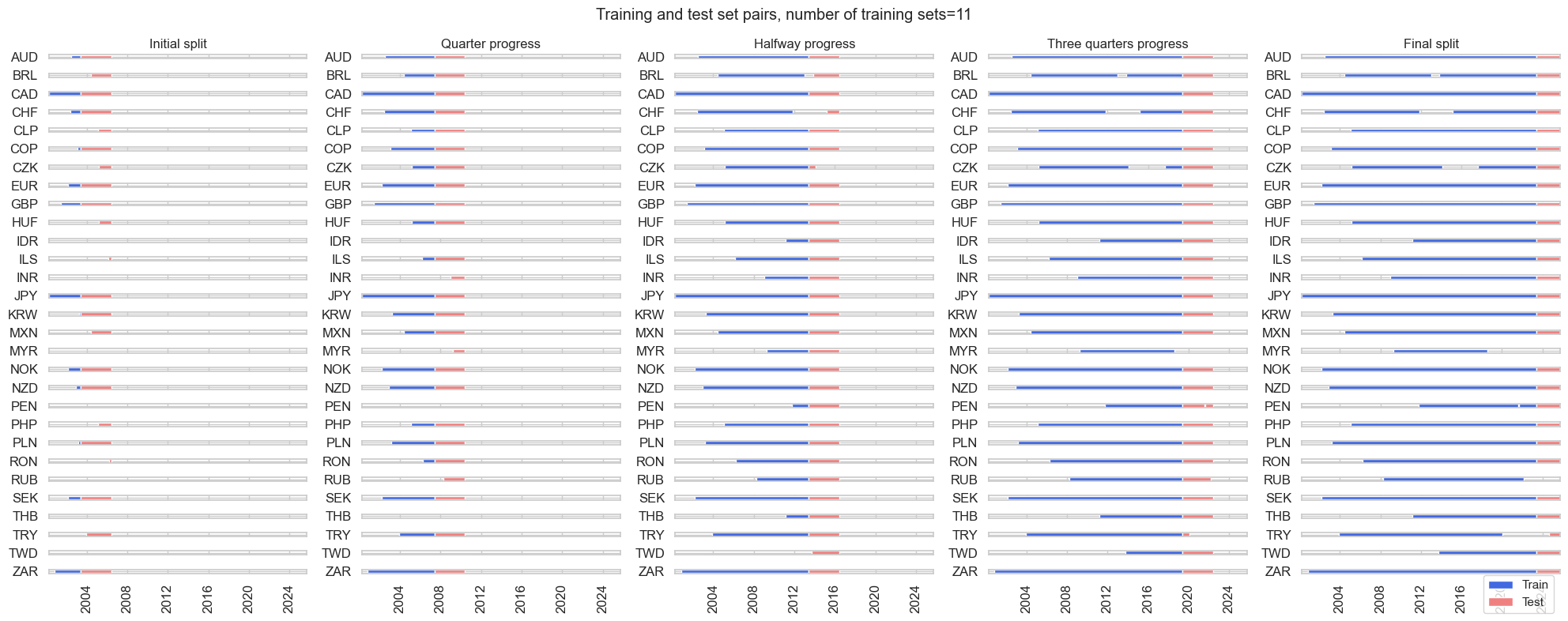
Cross-validation dynamics #
# Choose dynamic splitter with longer average

inner_splitter = {
    "Expanding": msl.ExpandingIncrementPanelSplit(
        train_intervals=24, test_size=36, min_cids=4, min_periods=24
    ),
}

# Visualize the validation procedure as run today
inner_splitter["Expanding"].visualise_splits(X_fx, y_fx, figsize=(20, 8))
A binary Sharpe ratio is used to evaluate a model in each cross-validation fold. This is aggregated across cross-validation folds by the mean Sharpe minus its standard deviation. This is done to encourage selection of a stable model across economic conditions.
# Choose scorer for cross-validation

scorer = {"SHARPE": make_scorer(msl.sharpe_ratio)}

# Specify how to aggregate metrics across cv folds

cv_summary = lambda row: np.nanmean(row) - np.nanstd(row)
Global FX signals #
Global instance of signal optimizer #
so_glb = msl.SignalOptimizer(
    df=dfx,
    xcats=fx_factz + ["FXXR_VT10"],
    cids=cids_fx,
    blacklist=fxblack,
)
Below are the global parameters that define the back tests that SignalOptimizer generates.
min_cids = 4
min_periods = 36
test_size = 12
Learning with ridge regressions #
Ridge without Adaboost #
so_glb.calculate_predictions(
    name="RIDGE",
    models={
        "RIDGE": Ridge(positive=True),
    },
    hyperparameters={
        "RIDGE": {
            "fit_intercept": [True, False],
            "alpha": [1, 10, 100, 1000, 10000],
        },
    },
    scorers=scorer,
    inner_splitters=inner_splitter,
    test_size=test_size,
    min_cids=min_cids,
    min_periods=min_periods,
    cv_summary=cv_summary,
)
dfa = so_glb.get_optimized_signals("RIDGE")
dfx = msm.update_df(dfx, dfa)
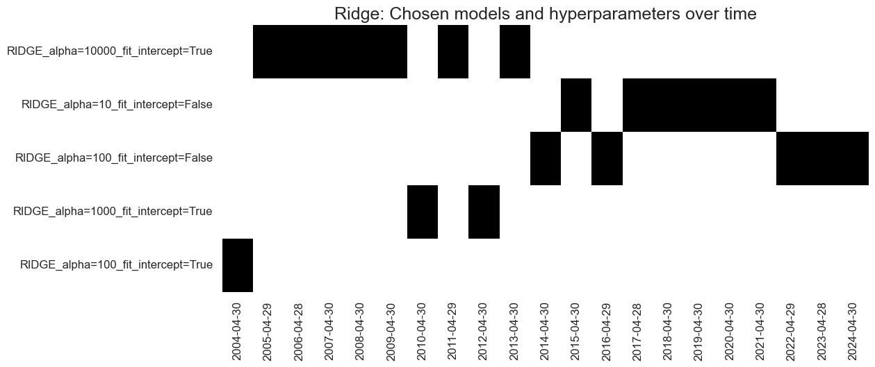
# Visualize hyperparameter choice
so_glb.models_heatmap(
"RIDGE",
title="Ridge: Chosen models and hyperparameters over time",
title_fontsize=18,
figsize=(12, 5)
)
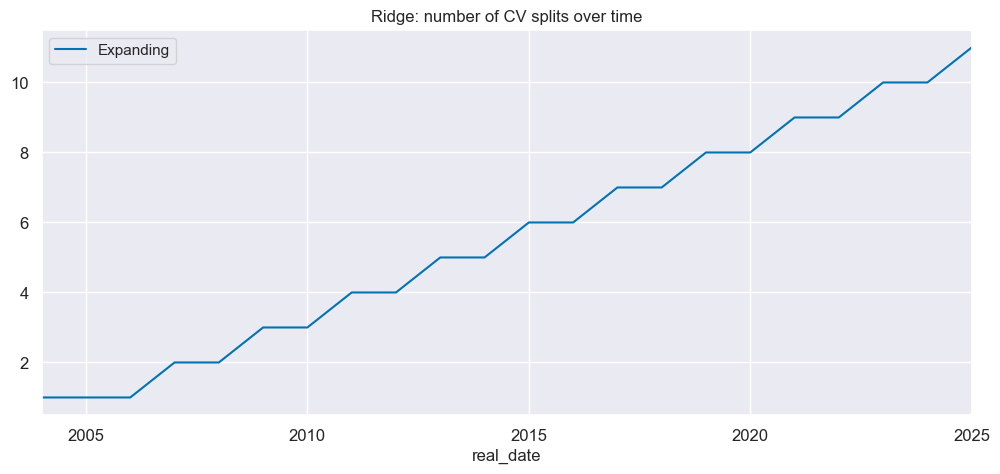
# Visualize growing number of CV splitters
so_glb.nsplits_timeplot(
"RIDGE",
title="Ridge: number of CV splits over time",
figsize=(12, 5)
)
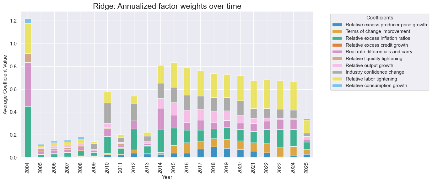
# Feature importance graph
so_glb.coefs_stackedbarplot(
"RIDGE",
title = "Ridge: Annualized factor weights over time",
title_fontsize = 18,
figsize=(14, 6),
ftrs_renamed=dict_factz
)
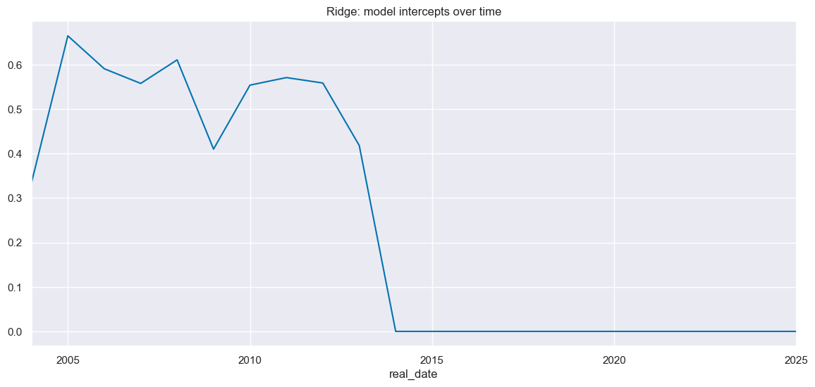
# Intercept choice
so_glb.intercepts_timeplot(
"RIDGE",
title = "Ridge: model intercepts over time",
figsize=(14, 6)
)
Ridge with Adaboost #
so_glb.calculate_predictions(
    name="ADA_RIDGE",
    models={
        "ADA_RIDGE": AdaBoostRegressor(
            estimator=msl.FIExtractor(Ridge(positive=True)),
            random_state=RANDOM_STATE,
            n_estimators=50,
        ),
        "RIDGE": msl.FIExtractor(Ridge(positive=True)),
    },
    hyperparameters={
        "ADA_RIDGE": {
            "estimator__estimator__fit_intercept": [True, False],
            "estimator__estimator__alpha": [1, 10, 100, 1000, 10000],
            "learning_rate": [1e-2, 1e-1, 1],
        },
        "RIDGE": {
            "estimator__fit_intercept": [True, False],
            "estimator__alpha": [1, 10, 100, 1000, 10000],
        },
    },
    scorers=scorer,
    inner_splitters=inner_splitter,
    test_size=test_size,
    cv_summary=cv_summary,
    min_cids=min_cids,
    min_periods=min_periods,
)
dfa = so_glb.get_optimized_signals("ADA_RIDGE")
dfx = msm.update_df(dfx, dfa)
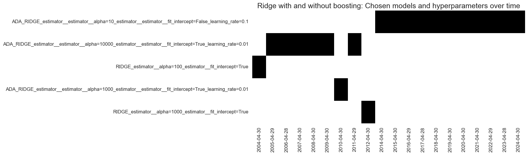
-
Initial preference for unboosted Ridge or boosting with small learning rates (very little adjustment and with large regularization).
-
Transition into more comprehensive boosting as more data is made available.
# Visualize hyperparameter choice
so_glb.models_heatmap(
    "ADA_RIDGE",
    title="Ridge with and without boosting: Chosen models and hyperparameters over time",
    title_fontsize=18,
    figsize=(12, 5)
)
-
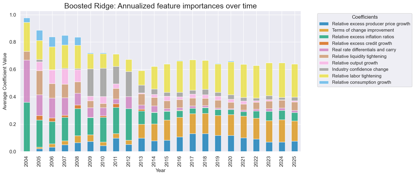
Consistent factor exposures with convergence to labor market tightening and terms-of-trade.
# Feature importance graph
so_glb.coefs_stackedbarplot(
    "ADA_RIDGE",
    title = "Boosted Ridge: Annualized feature importances over time",
    title_fontsize = 18,
    figsize=(14, 6),
    ftrs_renamed=dict_factz
)
Ridge value generation #
sigx = ["RIDGE", "ADA_RIDGE"]
pnl = msn.NaivePnL(
df=dfx,
ret="FXXR_VT10",
sigs=sigx,
blacklist=fxblack,
start="2004-04-30",
cids=cids_fx,
bms=["EUR_FXXR_NSA", "USD_EQXR_NSA"],
)
for xcat in sigx:
pnl.make_pnl(
sig=xcat,
sig_op="zn_score_pan",
rebal_freq="monthly",
rebal_slip=1,
vol_scale=10,
thresh=3,
)
pnl.make_long_pnl(label="LONG", vol_scale=10)
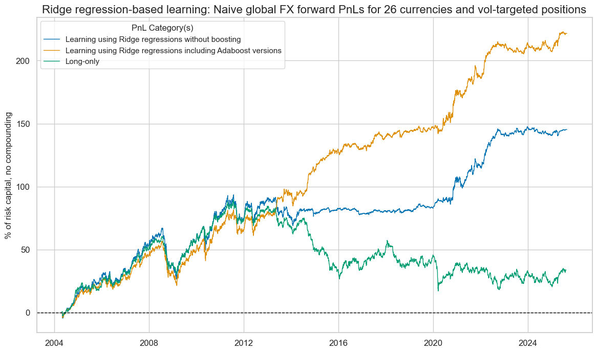
pnl.plot_pnls(
pnl_cats=["PNL_RIDGE", "PNL_ADA_RIDGE", "LONG"],
title="Ridge regression-based learning: Naive global FX forward PnLs for 26 currencies and vol-targeted positions",
title_fontsize=16,
xcat_labels=[
"Learning using Ridge regressions without boosting",
"Learning using Ridge regressions including Adaboost versions",
"Long-only",
],
figsize=(14, 8),
)
pnl.evaluate_pnls(pnl_cats=pnl.pnl_names)
| xcat | PNL_RIDGE | PNL_ADA_RIDGE | LONG |
|---|---|---|---|
| Return % | 6.812889 | 10.392827 | 1.590108 |
| St. Dev. % | 10.0 | 10.0 | 10.0 |
| Sharpe Ratio | 0.681289 | 1.039283 | 0.159011 |
| Sortino Ratio | 0.955954 | 1.513883 | 0.217356 |
| Max 21-Day Draw % | -18.898477 | -17.584196 | -21.939666 |
| Max 6-Month Draw % | -33.310015 | -28.709281 | -25.589386 |
| Peak to Trough Draw % | -40.459371 | -35.062344 | -72.308131 |
| Top 5% Monthly PnL Share | 0.656502 | 0.499743 | 2.581361 |
| EUR_FXXR_NSA correl | 0.358928 | 0.393527 | 0.498466 |
| USD_EQXR_NSA correl | 0.266557 | 0.253598 | 0.326144 |
| Traded Months | 257 | 257 | 257 |
DM and EM comparison #
sigx = ["RIDGE", "ADA_RIDGE"]
pnl = msn.NaivePnL(
df=dfx,
ret="FXXR_VT10",
sigs=sigx,
blacklist=fxblack,
start="2004-04-30",
cids=cids_dmfx,
bms=["EUR_FXXR_NSA", "USD_EQXR_NSA"],
)
for xcat in sigx:
pnl.make_pnl(
sig=xcat,
sig_op="zn_score_pan",
rebal_freq="monthly",
rebal_slip=1,
vol_scale=10,
thresh=3,
)
pnl.make_long_pnl(label="LONG", vol_scale=10)
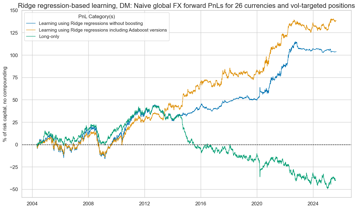
pnl.plot_pnls(
pnl_cats=["PNL_RIDGE", "PNL_ADA_RIDGE", "LONG"],
title="Ridge regression-based learning, DM: Naive global FX forward PnLs for 26 currencies and vol-targeted positions",
title_fontsize=16,
xcat_labels=[
"Learning using Ridge regressions without boosting",
"Learning using Ridge regressions including Adaboost versions",
"Long-only",
],
figsize=(14, 8),
)
pnl.evaluate_pnls(pnl_cats=pnl.pnl_names)
| xcat | PNL_RIDGE | PNL_ADA_RIDGE | LONG |
|---|---|---|---|
| Return % | 4.864647 | 6.487323 | -1.873782 |
| St. Dev. % | 10.0 | 10.0 | 10.0 |
| Sharpe Ratio | 0.486465 | 0.648732 | -0.187378 |
| Sortino Ratio | 0.695444 | 0.949653 | -0.259335 |
| Max 21-Day Draw % | -15.040752 | -11.86937 | -18.597592 |
| Max 6-Month Draw % | -32.234893 | -25.47533 | -27.286586 |
| Peak to Trough Draw % | -36.153225 | -28.572126 | -93.991435 |
| Top 5% Monthly PnL Share | 0.863884 | 0.784391 | -1.916001 |
| EUR_FXXR_NSA correl | 0.373075 | 0.473148 | 0.586398 |
| USD_EQXR_NSA correl | 0.116536 | 0.132292 | 0.187183 |
| Traded Months | 257 | 257 | 257 |
sigx = ["RIDGE", "ADA_RIDGE"]
pnl = msn.NaivePnL(
df=dfx,
ret="FXXR_VT10",
sigs=sigx,
blacklist=fxblack,
start="2004-04-30",
cids=cids_emfx,
bms=["EUR_FXXR_NSA", "USD_EQXR_NSA"],
)
for xcat in sigx:
pnl.make_pnl(
sig=xcat,
sig_op="zn_score_pan",
rebal_freq="monthly",
rebal_slip=1,
vol_scale=10,
thresh=3,
)
pnl.make_long_pnl(label="LONG", vol_scale=10)
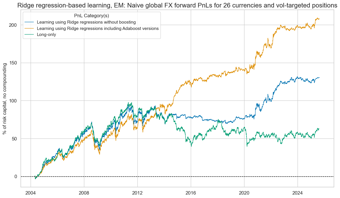
pnl.plot_pnls(
pnl_cats=["PNL_RIDGE", "PNL_ADA_RIDGE", "LONG"],
title="Ridge regression-based learning, EM: Naive global FX forward PnLs for 26 currencies and vol-targeted positions",
title_fontsize=16,
xcat_labels=[
"Learning using Ridge regressions without boosting",
"Learning using Ridge regressions including Adaboost versions",
"Long-only",
],
figsize=(14, 8),
)
pnl.evaluate_pnls(pnl_cats=pnl.pnl_names)
| xcat | PNL_RIDGE | PNL_ADA_RIDGE | LONG |
|---|---|---|---|
| Return % | 6.112908 | 9.744231 | 2.973157 |
| St. Dev. % | 10.0 | 10.0 | 10.0 |
| Sharpe Ratio | 0.611291 | 0.974423 | 0.297316 |
| Sortino Ratio | 0.85308 | 1.410505 | 0.405547 |
| Max 21-Day Draw % | -18.679799 | -16.930149 | -20.324754 |
| Max 6-Month Draw % | -29.83146 | -25.699652 | -24.494762 |
| Peak to Trough Draw % | -37.013071 | -32.10987 | -58.383761 |
| Top 5% Monthly PnL Share | 0.712341 | 0.483418 | 1.345372 |
| EUR_FXXR_NSA correl | 0.288561 | 0.260381 | 0.379631 |
| USD_EQXR_NSA correl | 0.282641 | 0.254126 | 0.340862 |
| Traded Months | 257 | 257 | 257 |
Learning with random forests #
Random forests without Adaboost #
so_glb.calculate_predictions(
    name="RF",
    models={
        "RF": RandomForestRegressor(
            n_estimators=100,
            max_samples = 0.1,
            monotonic_cst=[1 for i in range(len(fx_factz))],
            random_state=RANDOM_STATE,
        ),
    },
    hyperparameters={
        "RF": {
            "max_features": [0.3, 0.5],
        },
    },
    scorers=scorer,
    inner_splitters=inner_splitter,
    test_size=test_size,
    cv_summary=cv_summary,
    min_cids=min_cids,
    min_periods=min_periods,
)

dfa = so_glb.get_optimized_signals("RF")
dfx = msm.update_df(dfx, dfa)
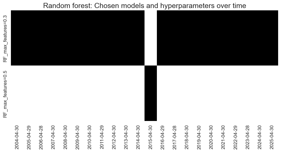
# Visualize hyperparameter choice
so_glb.models_heatmap(
    "RF",
    title="Random forest: Chosen models and hyperparameters over time",
    title_fontsize=18,
    figsize=(12, 5)
)
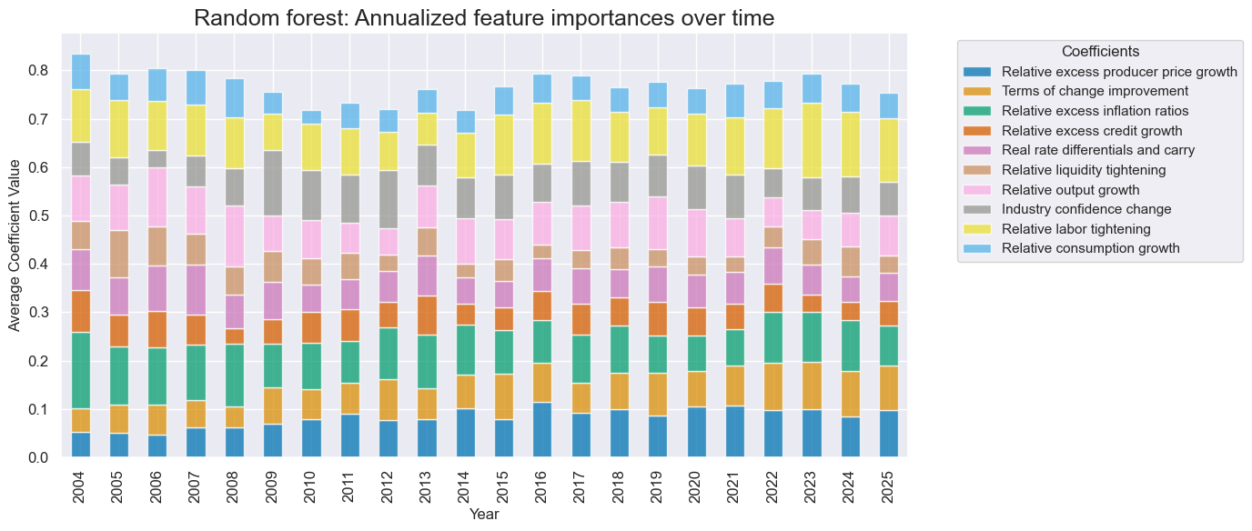
# Feature importance graph

so_glb.coefs_stackedbarplot(
    "RF",
    title = "Random forest: Annualized feature importances over time",
    title_fontsize = 18,
    figsize=(14, 6),
    ftrs_renamed=dict_factz
)
Random forests with Adaboost #
so_glb.calculate_predictions(
    name="ADA_RF",
    models={
        "ADA_RF": AdaBoostRegressor(
            estimator=RandomForestRegressor(
            n_estimators=100,
            max_samples = 0.1,
            monotonic_cst=[1 for i in range(len(fx_factz))],
        ),
            random_state=RANDOM_STATE,
            n_estimators=50,
        ),
        "RF": RandomForestRegressor(
            n_estimators=100,
            max_samples = 0.1,
            monotonic_cst=[1 for i in range(len(fx_factz))],
            random_state=RANDOM_STATE,
        ),
    },
    hyperparameters={
        "RF": {
            "max_features": [0.3, 0.5],
        },
        "ADA_RF": {
            "learning_rate": [1e-2, 1e-1, 1],
            "estimator__max_features": [0.3, 0.5],
        },
    },
    scorers=scorer,
    inner_splitters=inner_splitter,
    test_size=test_size,
    min_cids=min_cids,
    min_periods=min_periods,
    cv_summary=cv_summary,
)

dfa = so_glb.get_optimized_signals("ADA_RF")
dfx = msm.update_df(dfx, dfa)
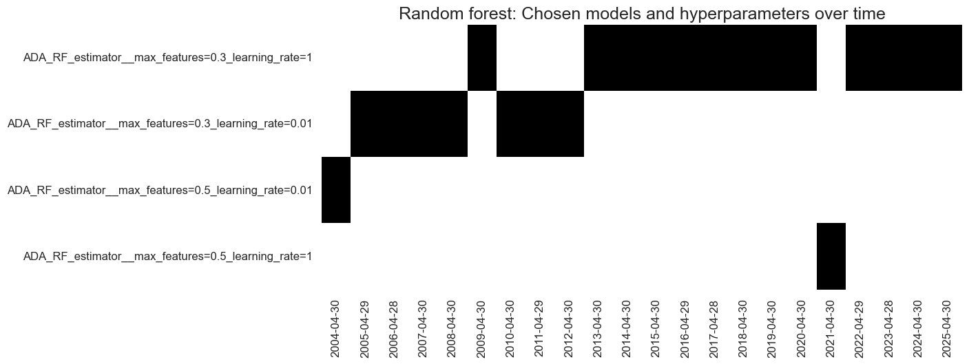
-
Again, earlier boosting is slight and becomes more aggressive over time, as data availability increases.
-
Favoured looser feature selection as data availability increased. This encourages diversity in the forest.
# Visualize hyperparameter choice
so_glb.models_heatmap(
    "ADA_RF",
    title="Random forest: Chosen models and hyperparameters over time",
    title_fontsize=18,
    figsize=(12, 5)
)
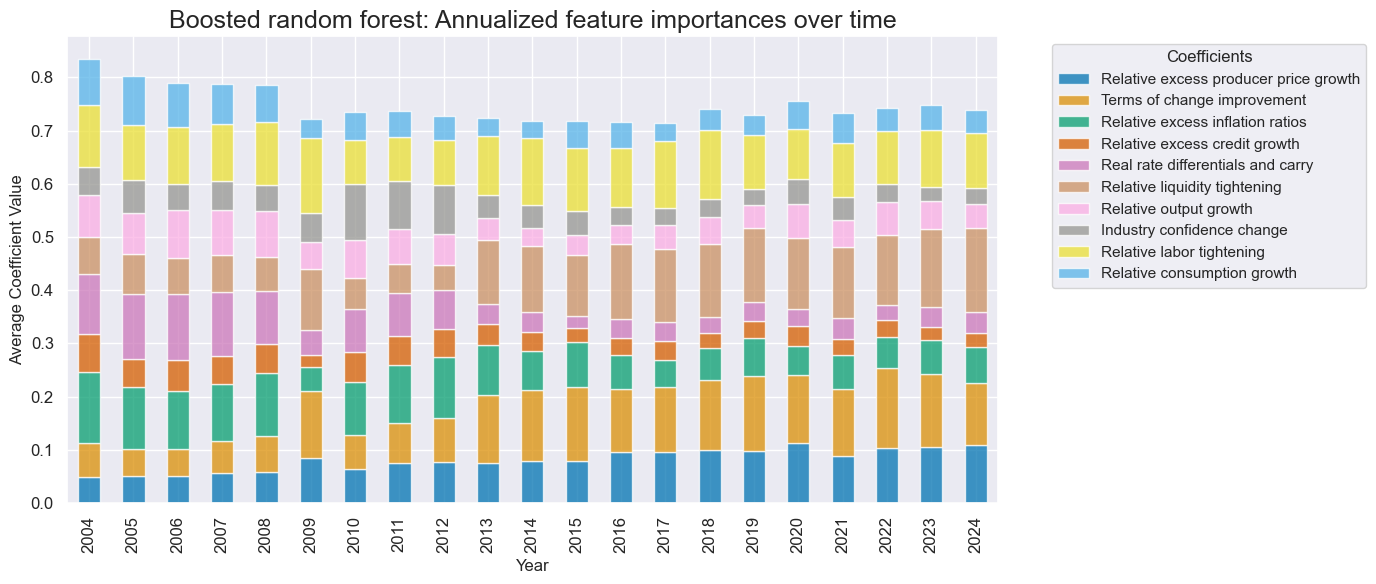
# Feature importance graph

so_glb.coefs_stackedbarplot(
    "ADA_RF",
    title="Boosted random forest: Annualized feature importances over time",
    title_fontsize=18,
    figsize=(14, 6),
    ftrs_renamed=dict_factz,
)
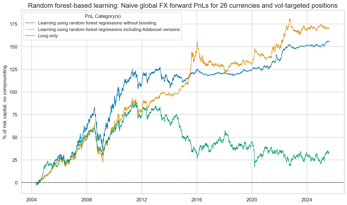
Random forest value generation #
-
Higher PnL generation from boosting came at the price of noise.
-
This indicates incorrect learning rate specification; the grid should be made finer.
sigx = ["RF", "ADA_RF"]

pnl = msn.NaivePnL(
    df=dfx,
    ret="FXXR_VT10",
    sigs=sigx,
    blacklist=fxblack,
    start="2004-04-30",
    cids=cids_fx,
    bms=["EUR_FXXR_NSA", "USD_EQXR_NSA"],
)

for xcat in sigx:
    pnl.make_pnl(
        sig=xcat,
        sig_op="zn_score_pan",
        rebal_freq="monthly",
        rebal_slip=1,
        vol_scale=10,
        thresh=2,
    )

pnl.make_long_pnl(label="LONG", vol_scale=10)

pnl.plot_pnls(
    pnl_cats=["PNL_RF", "PNL_ADA_RF", "LONG"],
    title="Random forest-based learning: Naive global FX forward PnLs for 26 currencies and vol-targeted positions",
    title_fontsize=16,
    xcat_labels=[
        "Learning using random forest regressions without boosting",
        "Learning using random forest regressions including Adaboost versions",
        "Long-only",
    ],
    figsize=(14, 8),
)
pnl.evaluate_pnls(pnl_cats=pnl.pnl_names)
| xcat | PNL_RF | PNL_ADA_RF | LONG |
|---|---|---|---|
| Return % | 7.317633 | 7.970184 | 1.590108 |
| St. Dev. % | 10.0 | 10.0 | 10.0 |
| Sharpe Ratio | 0.731763 | 0.797018 | 0.159011 |
| Sortino Ratio | 1.034682 | 1.154637 | 0.217356 |
| Max 21-Day Draw % | -19.166391 | -17.723897 | -21.939666 |
| Max 6-Month Draw % | -36.888144 | -33.801125 | -25.589386 |
| Peak to Trough Draw % | -46.909717 | -42.073355 | -72.308131 |
| Top 5% Monthly PnL Share | 0.651763 | 0.610813 | 2.581361 |
| EUR_FXXR_NSA correl | 0.31033 | 0.072472 | 0.498466 |
| USD_EQXR_NSA correl | 0.282191 | 0.086341 | 0.326144 |
| Traded Months | 257 | 257 | 257 |
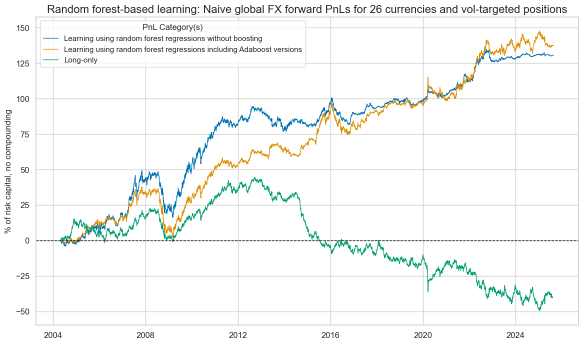
DM and EM comparison #
-
DM performance boosted but the noise comes from EM.
-
Supports theory of too high learning rates; attempting too much EM over-correction.
-
Raises question on whether it is more valuable to produce DM/EM-only signals based on DM/EM-only data or more valuable to train globally and restrict analysis to DM/EM.
-
Boosted random forests achieved lower correlations with EUR-USD excess FX returns than the boosted ridges.
sigx = ["RF", "ADA_RF"]

pnl = msn.NaivePnL(
    df=dfx,
    ret="FXXR_VT10",
    sigs=sigx,
    blacklist=fxblack,
    start="2004-04-30",
    cids=cids_dmfx,
    bms=["EUR_FXXR_NSA", "USD_EQXR_NSA"],
)

for xcat in sigx:
    pnl.make_pnl(
        sig=xcat,
        sig_op="zn_score_pan",
        rebal_freq="monthly",
        rebal_slip=1,
        vol_scale=10,
        thresh=2,
    )

pnl.make_long_pnl(label="LONG", vol_scale=10)

pnl.plot_pnls(
    pnl_cats=["PNL_RF", "PNL_ADA_RF", "LONG"],
    title="Random forest-based learning: Naive global FX forward PnLs for 26 currencies and vol-targeted positions",
    title_fontsize=16,
    xcat_labels=[
        "Learning using random forest regressions without boosting",
        "Learning using random forest regressions including Adaboost versions",
        "Long-only",
    ],
    figsize=(14, 8),
)
pnl.evaluate_pnls(pnl_cats=pnl.pnl_names)
| xcat | PNL_RF | PNL_ADA_RF | LONG |
|---|---|---|---|
| Return % | 6.119173 | 6.433992 | -1.873782 |
| St. Dev. % | 10.0 | 10.0 | 10.0 |
| Sharpe Ratio | 0.611917 | 0.643399 | -0.187378 |
| Sortino Ratio | 0.8727 | 0.92888 | -0.259335 |
| Max 21-Day Draw % | -16.316119 | -17.868455 | -18.597592 |
| Max 6-Month Draw % | -28.17934 | -31.031625 | -27.286586 |
| Peak to Trough Draw % | -32.981545 | -35.300397 | -93.991435 |
| Top 5% Monthly PnL Share | 0.656754 | 0.639637 | -1.916001 |
| EUR_FXXR_NSA correl | 0.193762 | -0.0471 | 0.586398 |
| USD_EQXR_NSA correl | 0.149577 | 0.045482 | 0.187183 |
| Traded Months | 257 | 257 | 257 |
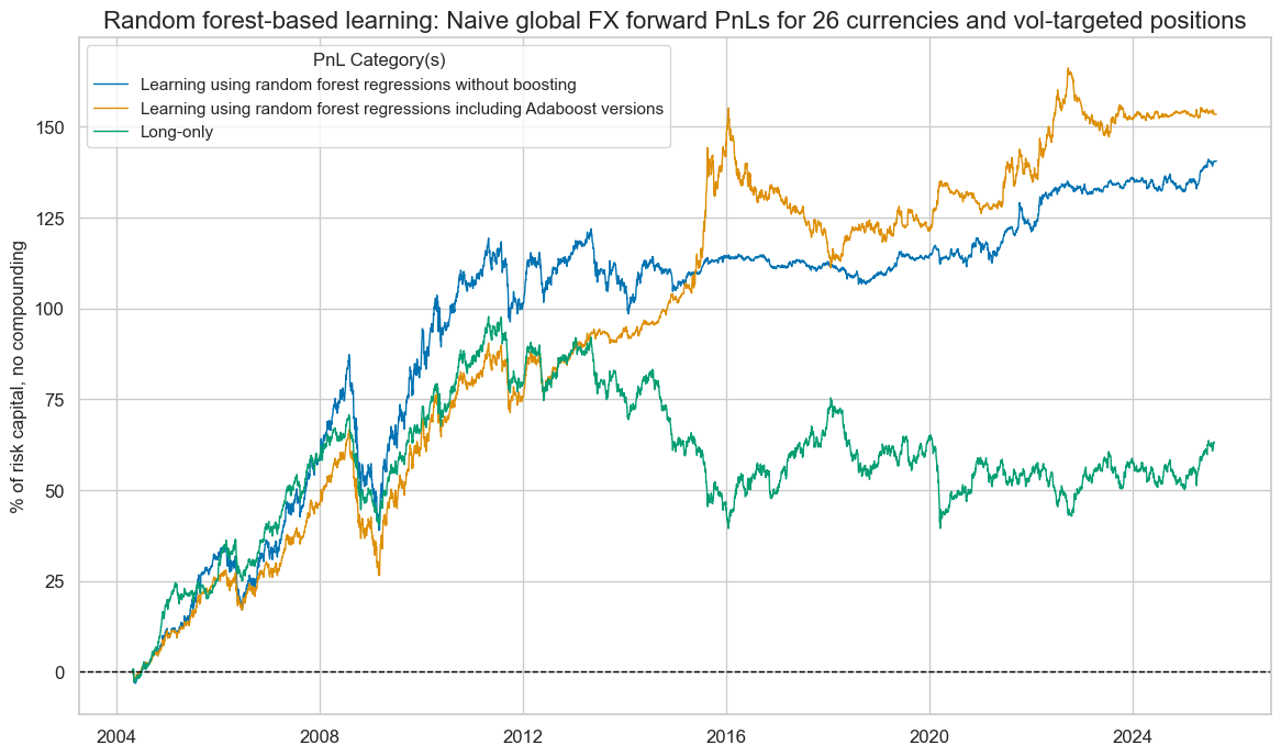
sigx = ["RF", "ADA_RF"]

pnl = msn.NaivePnL(
    df=dfx,
    ret="FXXR_VT10",
    sigs=sigx,
    blacklist=fxblack,
    start="2004-04-30",
    cids=cids_emfx,
    bms=["EUR_FXXR_NSA", "USD_EQXR_NSA"],
)

for xcat in sigx:
    pnl.make_pnl(
        sig=xcat,
        sig_op="zn_score_pan",
        rebal_freq="monthly",
        rebal_slip=1,
        vol_scale=10,
        thresh=2,
    )

pnl.make_long_pnl(label="LONG", vol_scale=10)

pnl.plot_pnls(
    pnl_cats=["PNL_RF", "PNL_ADA_RF", "LONG"],
    title="Random forest-based learning: Naive global FX forward PnLs for 26 currencies and vol-targeted positions",
    title_fontsize=16,
    xcat_labels=[
        "Learning using random forest regressions without boosting",
        "Learning using random forest regressions including Adaboost versions",
        "Long-only",
    ],
    figsize=(14, 8),
)
pnl.evaluate_pnls(pnl_cats=pnl.pnl_names)
| xcat | PNL_RF | PNL_ADA_RF | LONG |
|---|---|---|---|
| Return % | 6.590191 | 7.19554 | 2.973157 |
| St. Dev. % | 10.0 | 10.0 | 10.0 |
| Sharpe Ratio | 0.659019 | 0.719554 | 0.297316 |
| Sortino Ratio | 0.925645 | 1.041325 | 0.405547 |
| Max 21-Day Draw % | -18.007629 | -14.808436 | -20.324754 |
| Max 6-Month Draw % | -37.684207 | -30.938681 | -24.494762 |
| Peak to Trough Draw % | -48.365595 | -44.022846 | -58.383761 |
| Top 5% Monthly PnL Share | 0.724194 | 0.683142 | 1.345372 |
| EUR_FXXR_NSA correl | 0.309024 | 0.114917 | 0.379631 |
| USD_EQXR_NSA correl | 0.285383 | 0.08032 | 0.340862 |
| Traded Months | 257 | 257 | 257 |
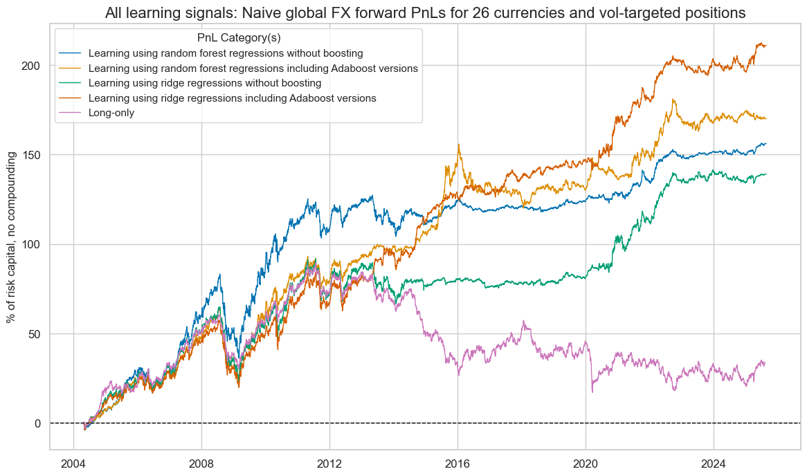
Comparison #
Both boosted models outperform their counterparts. The boosted forest and the boosted ridge model outperform at different times - and there are periods where they trade similarly. The random forest model has greater seasonality than the ridge model, but is virtually uncorrelated with the market.
sigx = ["RF", "ADA_RF", "RIDGE", "ADA_RIDGE"]

pnl = msn.NaivePnL(
    df=dfx,
    ret="FXXR_VT10",
    sigs=sigx,
    blacklist=fxblack,
    start="2004-04-30",
    cids=cids_fx,
    bms=["EUR_FXXR_NSA", "USD_EQXR_NSA"],
)

for xcat in sigx:
    pnl.make_pnl(
        sig=xcat,
        sig_op="zn_score_pan",
        rebal_freq="monthly",
        rebal_slip=1,
        vol_scale=10,
        thresh=2,
    )

pnl.make_long_pnl(label="LONG", vol_scale=10)

pnl.plot_pnls(
    pnl_cats=["PNL_RF", "PNL_ADA_RF", "PNL_RIDGE", "PNL_ADA_RIDGE", "LONG"],
    title="All learning signals: Naive global FX forward PnLs for 26 currencies and vol-targeted positions",
    title_fontsize=16,
    xcat_labels=[
        "Learning using random forest regressions without boosting",
        "Learning using random forest regressions including Adaboost versions",
        "Learning using ridge regressions without boosting",
        "Learning using ridge regressions including Adaboost versions",
        "Long-only",
    ],
    figsize=(14, 8),
)
pnl.evaluate_pnls(pnl_cats=pnl.pnl_names)
| xcat | PNL_RF | PNL_ADA_RF | PNL_RIDGE | PNL_ADA_RIDGE | LONG |
|---|---|---|---|---|---|
| Return % | 7.317633 | 7.970184 | 6.519403 | 9.889611 | 1.590108 |
| St. Dev. % | 10.0 | 10.0 | 10.0 | 10.0 | 10.0 |
| Sharpe Ratio | 0.731763 | 0.797018 | 0.65194 | 0.988961 | 0.159011 |
| Sortino Ratio | 1.034682 | 1.154637 | 0.912672 | 1.428918 | 0.217356 |
| Max 21-Day Draw % | -19.166391 | -17.723897 | -19.189374 | -18.614839 | -21.939666 |
| Max 6-Month Draw % | -36.888144 | -33.801125 | -33.886467 | -30.669504 | -25.589386 |
| Peak to Trough Draw % | -46.909717 | -42.073355 | -41.159548 | -37.456344 | -72.308131 |
| Top 5% Monthly PnL Share | 0.651763 | 0.610813 | 0.678857 | 0.490225 | 2.581361 |
| EUR_FXXR_NSA correl | 0.31033 | 0.072472 | 0.362705 | 0.405952 | 0.498466 |
| USD_EQXR_NSA correl | 0.282191 | 0.086341 | 0.26795 | 0.261157 | 0.326144 |
| Traded Months | 257 | 257 | 257 | 257 | 257 |