Dimension reduction and statistical learning #
Get packages and JPMaQS data #
Packages #
# >>> Define constants <<< #
import os

# Minimum Macrosynergy package version required for this notebook
MIN_REQUIRED_VERSION: str = "1.0.0"

# DataQuery credentials: Remember to replace with your own client ID and secret
DQ_CLIENT_ID: str = os.getenv("DQ_CLIENT_ID")
DQ_CLIENT_SECRET: str = os.getenv("DQ_CLIENT_SECRET")

# Define any Proxy settings required (http/https)
PROXY = {}

# Start date for the data (argument passed to the JPMaQSDownloader class)
START_DATE: str = "2000-01-01"
# Standard library imports
import numpy as np
import pandas as pd
import seaborn as sns
import warnings
from functools import partial
import itertools

# Scikit-learn imports
from sklearn.pipeline import Pipeline
from sklearn.decomposition import PCA
from sklearn.preprocessing import StandardScaler
from sklearn.compose import ColumnTransformer

from sklearn.metrics import make_scorer, root_mean_squared_error

# Macrosynergy package imports
import macrosynergy.management as msm
import macrosynergy.panel as msp
import macrosynergy.pnl as msn
import macrosynergy.signal as mss
import macrosynergy.learning as msl
import macrosynergy.visuals as msv
from macrosynergy.download import JPMaQSDownload

warnings.simplefilter("ignore")
# Check installed Macrosynergy package meets version requirement
import macrosynergy as msy

msy.check_package_version(required_version=MIN_REQUIRED_VERSION)
Data #
# IRS cross-section lists

cids_dm = [
    "AUD",
    "CAD",
    "CHF",
    "EUR",
    "GBP",
    "JPY",
    "NOK",
    "NZD",
    "SEK",
    "USD",
]  # DM currency areas

cids_iliq = [
    "NOK",
    "NZD",
]

cids = sorted(set(cids_dm) - set(cids_iliq))
# Category tickers

cpi = [
    # CPI inflation
    "CPIH_SA_P1M1ML12",
    "CPIH_SJA_P6M6ML6AR",
    "CPIC_SA_P1M1ML12",
    "CPIC_SJA_P6M6ML6AR",
    "INFE2Y_JA",
]
ppi = [
    # PPI inflation
    "PPIH_NSA_P1M1ML12_3MMA",
    "PPIH_SA_P6M6ML6AR",
    "PGDPTECH_SA_P1M1ML12_3MMA",
    "PGDP_SA_P1Q1QL4",
]
inf = cpi + ppi

dem = [
    # Domestic demand growth
    "RRSALES_SA_P1M1ML12_3MMA",
    "RRSALES_SA_P1Q1QL4",
    "RPCONS_SA_P1Q1QL4",
    "RPCONS_SA_P1M1ML12_3MMA",
    "IMPORTS_SA_P1M1ML12_3MMA",
]
out = [
    # Output growth
    "INTRGDP_NSA_P1M1ML12_3MMA",
    "RGDPTECH_SA_P1M1ML12_3MMA",
    "IP_SA_P1M1ML12_3MMA",
]
lab = [
    # Labour market tightening and tightness
    "EMPL_NSA_P1M1ML12_3MMA",
    "EMPL_NSA_P1Q1QL4",
    "UNEMPLRATE_NSA_3MMA_D1M1ML12",
    "UNEMPLRATE_NSA_D1Q1QL4",
    "UNEMPLRATE_SA_3MMAv5YMA",
    "WAGES_NSA_P1M1ML12_3MMA",
    "WAGES_NSA_P1Q1QL4",
]
ecg = dem + out + lab

mon = [
    # Money and liquidity growth
    "MNARROW_SJA_P1M1ML12",
    "MBROAD_SJA_P1M1ML12",
    "MBASEGDP_SA_D1M1ML6",
    "INTLIQGDP_NSA_D1M1ML6",
]
crh = [
    # Credit and housing market
    "PCREDITBN_SJA_P1M1ML12",
    "PCREDITGDP_SJA_D1M1ML12",
    "HPI_SA_P1M1ML12_3MMA",
    "HPI_SA_P1Q1QL4",
]
mcr = mon + crh

main = inf + ecg + mcr

adds = [
    # Additional variables for benchmark calculation
    "RGDP_SA_P1Q1QL4_20QMM",
    "INFTEFF_NSA",
    "WFORCE_NSA_P1Y1YL1_5YMM",
    "WFORCE_NSA_P1Q1QL4_20QMM",
]

ecos = main + adds

rets = [
    # Target returns
    "DU05YXR_VT10",
    "DU05YXR_NSA",
]

xcats = ecos + rets

# Asset return tickers for benchmark correlation analysis
xtra = ["USD_EQXR_NSA", "USD_GB10YXR_NSA"]

tickers = [cid + "_" + xcat for cid in cids for xcat in xcats] + xtra
# Download series from J.P. Morgan DataQuery by tickers

start_date = "2000-01-01"
print(f"Maximum number of tickers is {len(tickers)}")

# Retrieve credentials

client_id: str = os.getenv("DQ_CLIENT_ID")
client_secret: str = os.getenv("DQ_CLIENT_SECRET")

with JPMaQSDownload(client_id=client_id, client_secret=client_secret) as dq:
    df = dq.download(
        tickers=tickers,
        start_date=start_date,
        suppress_warning=True,
        metrics=["value"],
        report_time_taken=True,
        show_progress=True,
    )
Maximum number of tickers is 306
Downloading data from JPMaQS.
Timestamp UTC:  2025-09-11 13:13:39
Connection successful!
Requesting data: 100%|██████████████████████████| 16/16 [00:03<00:00,  4.84it/s]
Downloading data: 100%|█████████████████████████| 16/16 [00:15<00:00,  1.05it/s]
Time taken to download data: 	19.78 seconds.
Some expressions are missing from the downloaded data. Check logger output for complete list.
56 out of 306 expressions are missing. To download the catalogue of all available expressions and filter the unavailable expressions, set `get_catalogue=True` in the call to `JPMaQSDownload.download()`.
dfx = df.copy()
dfx.info()
<class 'pandas.core.frame.DataFrame'>
RangeIndex: 1657842 entries, 0 to 1657841
Data columns (total 4 columns):
 #   Column     Non-Null Count    Dtype
---  ------     --------------    -----
 0   real_date  1657842 non-null  datetime64[ns]
 1   cid        1657842 non-null  object
 2   xcat       1657842 non-null  object
 3   value      1657842 non-null  float64
dtypes: datetime64[ns](1), float64(1), object(2)
memory usage: 50.6+ MB
Renaming and availability #
Renaming #
dict_repl = {
    # Wages
    "WAGES_NSA_P1Q1QL4": "WAGES_NSA_P1M1ML12_3MMA",
    # House prices
    "HPI_SA_P1Q1QL4": "HPI_SA_P1M1ML12_3MMA",
    # Labour market
    "EMPL_NSA_P1Q1QL4": "EMPL_NSA_P1M1ML12_3MMA",
    "UNEMPLRATE_NSA_D1Q1QL4": "UNEMPLRATE_NSA_3MMA_D1M1ML12",
    "UNEMPLRATE_SA_D2Q2QL2": "UNEMPLRATE_SA_D6M6ML6",
    # Other
    "RRSALES_SA_P1Q1QL4": "RRSALES_SA_P1M1ML12_3MMA",
    "RPCONS_SA_P1Q1QL4": "RPCONS_SA_P1M1ML12_3MMA",
    "WFORCE_NSA_P1Y1YL1_5YMM": "WFORCE_NSA_P1Q1QL4_20QMM",
}

for key, value in dict_repl.items():
    dfx["xcat"] = dfx["xcat"].str.replace(key, value)


eco_lists = [inf, ecg, mcr, adds]  # remove replaced tickers from economic concept lists
for i in range(len(eco_lists)):
    eco_lists[i][:] = [xc for xc in eco_lists[i] if xc in dfx["xcat"].unique()]
Check availability #
xcatx = inf
msm.check_availability(df=dfx, xcats=xcatx, cids=cids, missing_recent=False)
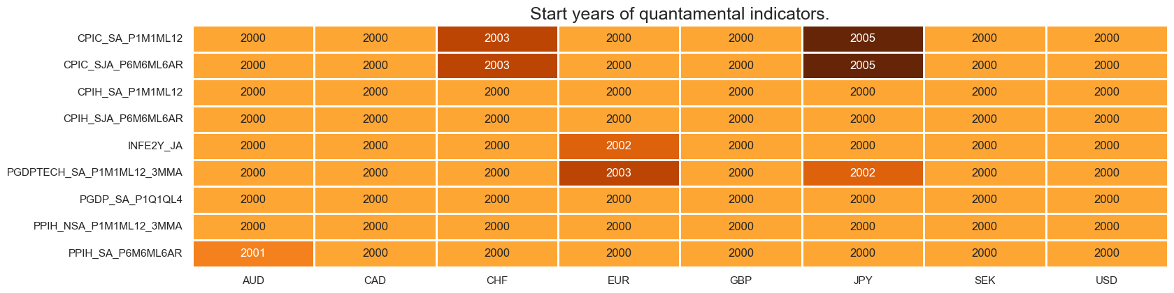
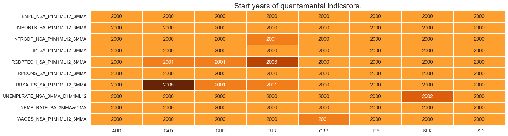
xcatx = ecg
msm.check_availability(df=dfx, xcats=xcatx, cids=cids, missing_recent=False)
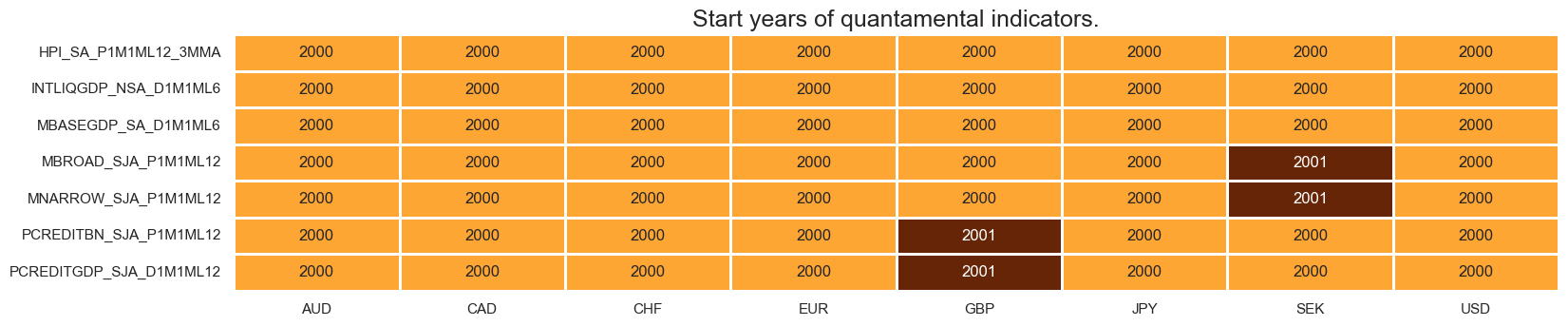
xcatx = mcr
msm.check_availability(df=dfx, xcats=xcatx, cids=cids, missing_recent=False)
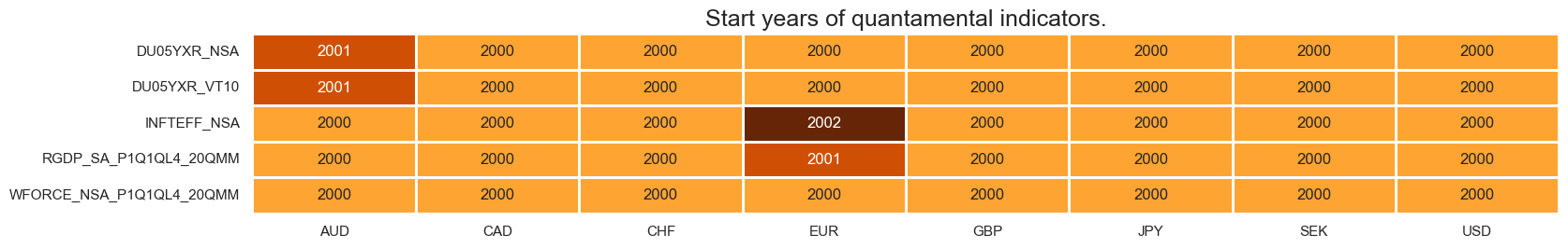
xcatx = adds + rets
msm.check_availability(df=dfx, xcats=xcatx, cids=cids, missing_recent=False)
Transformation and checks #
dict_labels = {}
dict_factorz = {}
Inflation shortfall #
# All excess inflation rates

xcatx = inf

dfa = msp.panel_calculator(
    df=dfx, calcs=[f"X{xcat}N = - {xcat} + INFTEFF_NSA" for xcat in xcatx], cids=cids
)
dfx = msm.update_df(dfx, dfa)

xinf = [f"X{xcat}N" for xcat in inf]
# Category-wise sequential normalization

xcatx = xinf

for xcat in xcatx:
    dfa = msp.make_zn_scores(
        df=dfx,
        xcat=xcat,
        cids=cids,
        neutral="zero",
        thresh=3,
        est_freq="M",
        pan_weight=1,
        postfix="_ZN",
    )
    dfx = msm.update_df(dfx, dfa)

# Labels

dict_labels["XCPIH_SA_P1M1ML12N_ZN"] = "CPI, %oya, excess, negative"
dict_labels["XCPIH_SJA_P6M6ML6ARN_ZN"] = "CPI, %6m/6m, saar, excess, negative"
dict_labels["XCPIC_SA_P1M1ML12N_ZN"] = "Core CPI, %oya, excess, negative"
dict_labels["XCPIC_SJA_P6M6ML6ARN_ZN"] = "Core CPI, %6m/6m, saar, excess, negative"
dict_labels["XINFE2Y_JAN_ZN"] = "CPI inflation expectations, excess, negative"
dict_labels["XPPIH_NSA_P1M1ML12_3MMAN_ZN"] = "PPI, %oya, 3mma, excess, negative"
dict_labels["XPPIH_SA_P6M6ML6ARN_ZN"] = "PPI, %6m/6m, saar, excess, negative"
dict_labels["XPGDPTECH_SA_P1M1ML12_3MMAN_ZN"] = "GDP deflator nowcast, %oya, 3mma, excess, negative"
dict_labels["XPGDP_SA_P1Q1QL4N_ZN"] = "GDP deflator, %oya, excess, negative"

# Factors

dict_factorz["XCPINZ"] = [f"X{xcat}N_ZN" for xcat in cpi]
dict_factorz["XPPINZ"] = [f"X{xcat}N_ZN" for xcat in ppi]
dict_factorz["XINFNZ_BROAD"] = [f"X{xcat}N_ZN" for xcat in inf]
# Visual check of factor groups
factor = "XINFNZ_BROAD" # XCPINZ, XPPINZ, XINFNZ_BROAD
xcatx = dict_factorz[factor]
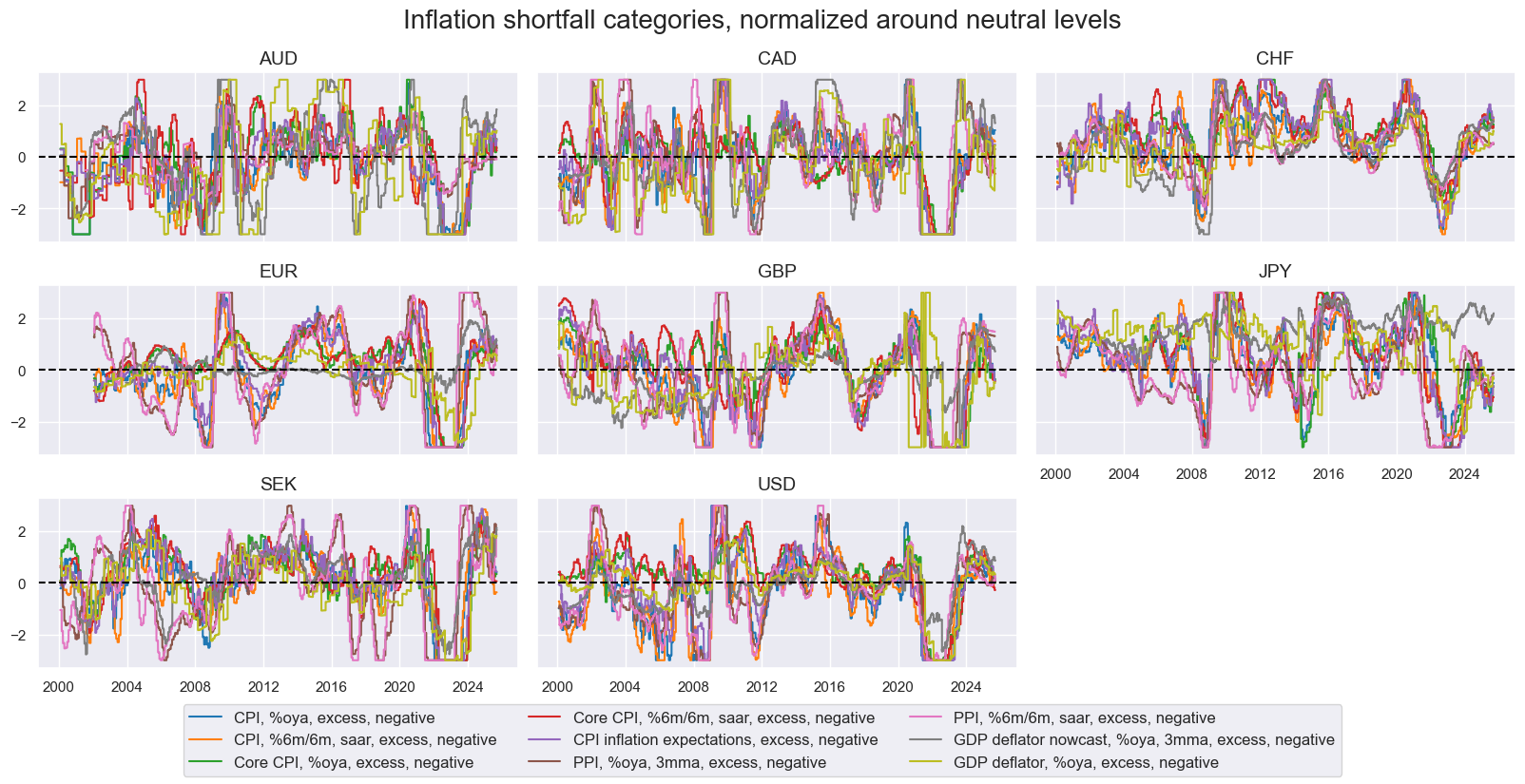
msp.view_timelines(
dfx,
xcats=xcatx,
cids=cids,
ncol=3,
aspect=2,
height=1.8,
start="2000-01-01",
same_y=True,
title="Inflation shortfall categories, normalized around neutral levels",
title_fontsize=20,
xcat_labels=dict_labels,
)
height = len(xcatx)
width = round(height * 1.5)
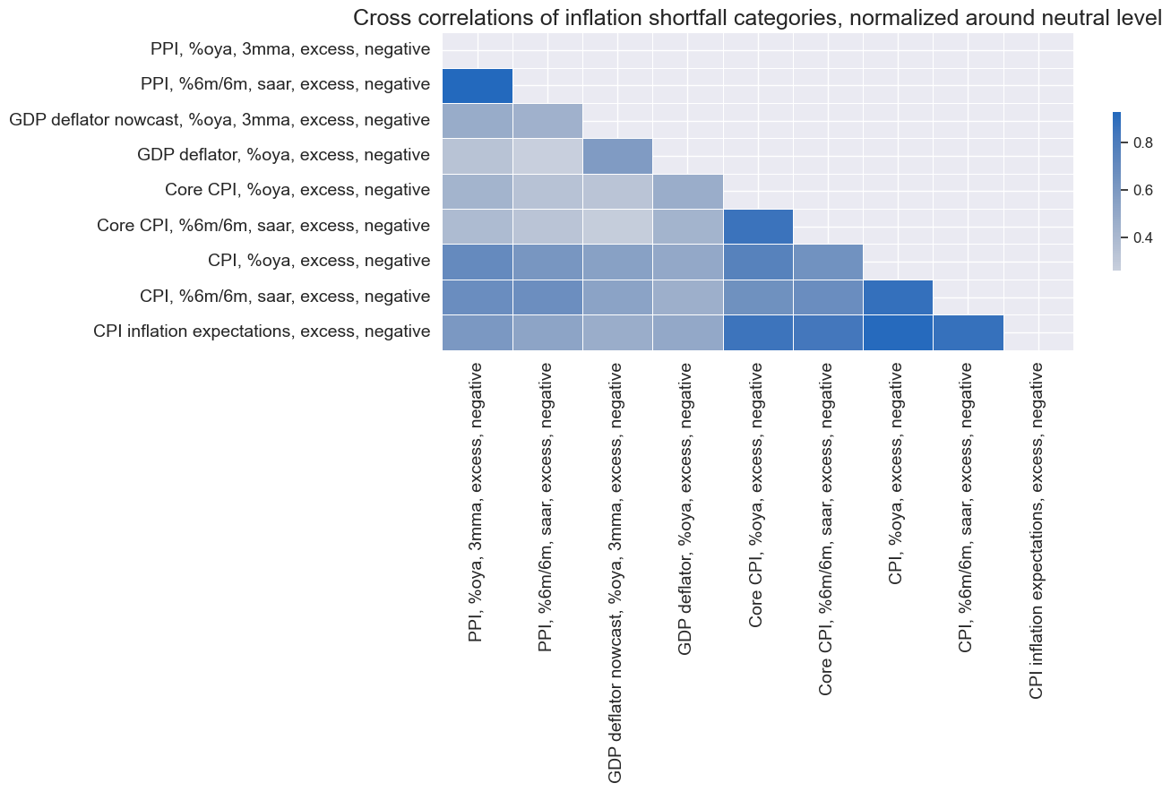
msp.correl_matrix(
dfx,
xcats=xcatx,
cids=cids,
freq="M",
size=(width, height),
cluster=True,
title="Cross correlations of inflation shortfall categories, normalized around neutral level",
title_fontsize=18,
xcat_labels={xcat:dict_labels[xcat] for xcat in xcatx},
)
Economic activity shortfall #
# All excess activity growth rates

act = [xcat for xcat in ecg if xcat in dem + out]
xcatx = act

dfa = msp.panel_calculator(
    df=dfx,
    calcs=[f"X{xcat}N = - {xcat} + RGDP_SA_P1Q1QL4_20QMM" for xcat in xcatx],
    cids=cids,
)
dfx = msm.update_df(dfx, dfa)

xact = ["X" + xcat + "N" for xcat in act]
# Excess employment, excess wage growth and unemployment shortfalls

calcs = []
calcs += [
    "XEMPL_NSA_P1M1ML12_3MMAN = - EMPL_NSA_P1M1ML12_3MMA + WFORCE_NSA_P1Q1QL4_20QMM"
]
calcs += [
    "WAGEGROWTH_NEUTRAL = INFTEFF_NSA + RGDP_SA_P1Q1QL4_20QMM - WFORCE_NSA_P1Q1QL4_20QMM"
]
calcs += ["XWAGES_NSA_P1M1ML12_3MMAN = - WAGES_NSA_P1M1ML12_3MMA + WAGEGROWTH_NEUTRAL"]

dfa = msp.panel_calculator(df=dfx, calcs=calcs, cids=cids)
dfx = msm.update_df(dfx, dfa)

xoth = [xcat for xcat in list(dfa["xcat"].unique()) if xcat != "WAGEGROWTH_NEUTRAL"] + [
    "UNEMPLRATE_NSA_3MMA_D1M1ML12",
    "UNEMPLRATE_SA_3MMAv5YMA",
]
xecg = xact + xoth
# Category-wise sequential normalization

xcatx = xecg

for xcat in xcatx:
    dfa = msp.make_zn_scores(
        df=dfx,
        xcat=xcat,
        cids=cids,
        neutral="zero",
        thresh=3,
        est_freq="M",
        pan_weight=1,
        postfix="_ZN",
    )
    dfx = msm.update_df(dfx, dfa)

# Labels

dict_labels["XRRSALES_SA_P1M1ML12_3MMAN_ZN"] = "Retail sales, %oya, 3mma, excess, negative"
dict_labels["XRPCONS_SA_P1M1ML12_3MMAN_ZN"] = "Private consumption, %oya, 3mma, excess, negative"
dict_labels["XIMPORTS_SA_P1M1ML12_3MMAN_ZN"] = "Imports, %oya, 3mma, excess, negative"
dict_labels["XINTRGDP_NSA_P1M1ML12_3MMAN_ZN"] = "GDP, intuitive nowcast, %oya, 3mma, excess, negative"
dict_labels["XRGDPTECH_SA_P1M1ML12_3MMAN_ZN"] = "GDP, technical nowcast, %oya, 3mma, excess, negative"
dict_labels["XIP_SA_P1M1ML12_3MMAN_ZN"] = "Industrial production, %oya, 3mma, excess, negative"
dict_labels["XEMPL_NSA_P1M1ML12_3MMAN_ZN"] = "Employment, %oya, 3mma, excess, negative"
dict_labels["XWAGES_NSA_P1M1ML12_3MMAN_ZN"] = "Wages, %oya, 3mma, excess, negative"
dict_labels["UNEMPLRATE_NSA_3MMA_D1M1ML12_ZN"] = "Unemployment rate, diff oya, 3mma"
dict_labels["UNEMPLRATE_SA_3MMAv5YMA_ZN"] = "Unemployment rate, diff over 5yma"

# Factors

dict_factorz["XDEMNZ"] = [f"{xcat}_ZN" for xcat in xecg if any(s in xcat for s in dem)]
dict_factorz["XOUTNZ"] = [f"{xcat}_ZN" for xcat in xecg if any(s in xcat for s in out)]
dict_factorz["XLABNZ"] = [f"{xcat}_ZN" for xcat in xecg if any(s in xcat for s in lab)]
dict_factorz["XECGNZ_BROAD"] = [
    f"{xcat}_ZN" for xcat in xecg if any(s in xcat for s in ecg)
]
# Visual check of factor groups
factor = "XECGNZ_BROAD" # XDEMNZ, XOUTNZ, XLABNZ, XECGNZ_BROAD
xcatx = dict_factorz[factor]
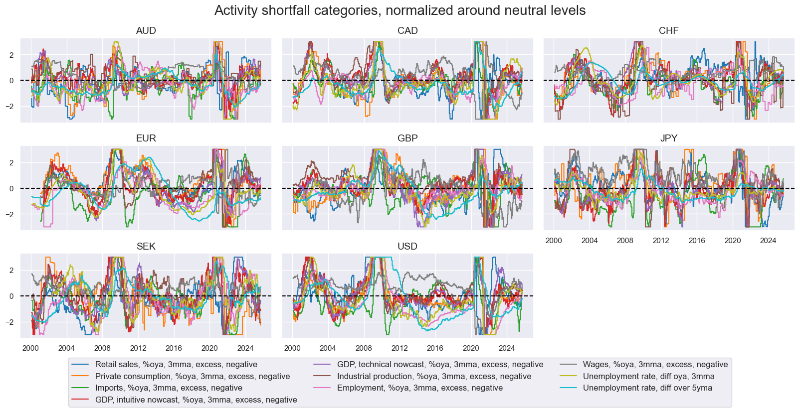
msp.view_timelines(
dfx,
xcats=xcatx,
cids=cids,
ncol=3,
aspect=2,
height=1.8,
start="2000-01-01",
same_y=True,
title="Activity shortfall categories, normalized around neutral levels",
title_fontsize=20,
xcat_labels=dict_labels,
)
height = len(xcatx)
width = round(height * 1.5)
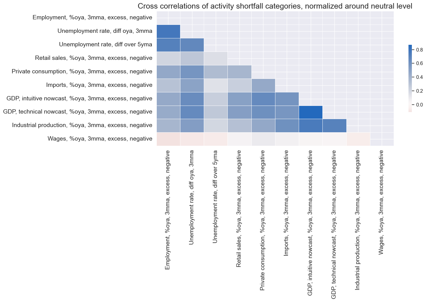
msp.correl_matrix(
dfx,
xcats=xcatx,
cids=cids,
freq="M",
size=(width, height),
cluster=True,
title="Cross correlations of activity shortfall categories, normalized around neutral level",
title_fontsize=18,
xcat_labels={xcat:dict_labels[xcat] for xcat in xcatx},
)
Excess money and credit growth #
# Excess money and credit growth rates

xcatx = [
    "MNARROW_SJA_P1M1ML12",
    "MBROAD_SJA_P1M1ML12",
    "PCREDITBN_SJA_P1M1ML12",
    "PCREDITGDP_SJA_D1M1ML12",
]

dfa = msp.panel_calculator(
    df=dfx,
    calcs=[
        f"X{xcat}N = - {xcat} + ( RGDP_SA_P1Q1QL4_20QMM + INFTEFF_NSA )"
        for xcat in xcatx
    ],
    cids=cids,
)
dfx = msm.update_df(dfx, dfa)

xmcr1 = ["X" + xcat + "N" for xcat in xcatx]
# Excess house price growth & pseudo excess liquidity growth

calcs = []
calcs += ["XHPI_SA_P1M1ML12_3MMAN = - HPI_SA_P1M1ML12_3MMA + INFTEFF_NSA"]
calcs += ["INTLIQGDP_NSA_D1M1ML6N = - INTLIQGDP_NSA_D1M1ML6"]
calcs += ["MBASEGDP_SA_D1M1ML6N = - MBASEGDP_SA_D1M1ML6"]

dfa = msp.panel_calculator(df=dfx, calcs=calcs, cids=cids)
dfx = msm.update_df(dfx, dfa)

xmcr2 = list(dfa["xcat"].unique())
xmcr = xmcr1 + xmcr2
# Category-wise sequential normalization
xcatx = xmcr
for xcat in xcatx:
dfa = msp.make_zn_scores(
df=dfx,
xcat=xcat,
cids=cids,
neutral="zero",
thresh=3,
est_freq="M",
pan_weight=1,
postfix="_ZN",
)
dfx = msm.update_df(dfx, dfa)
# Labels
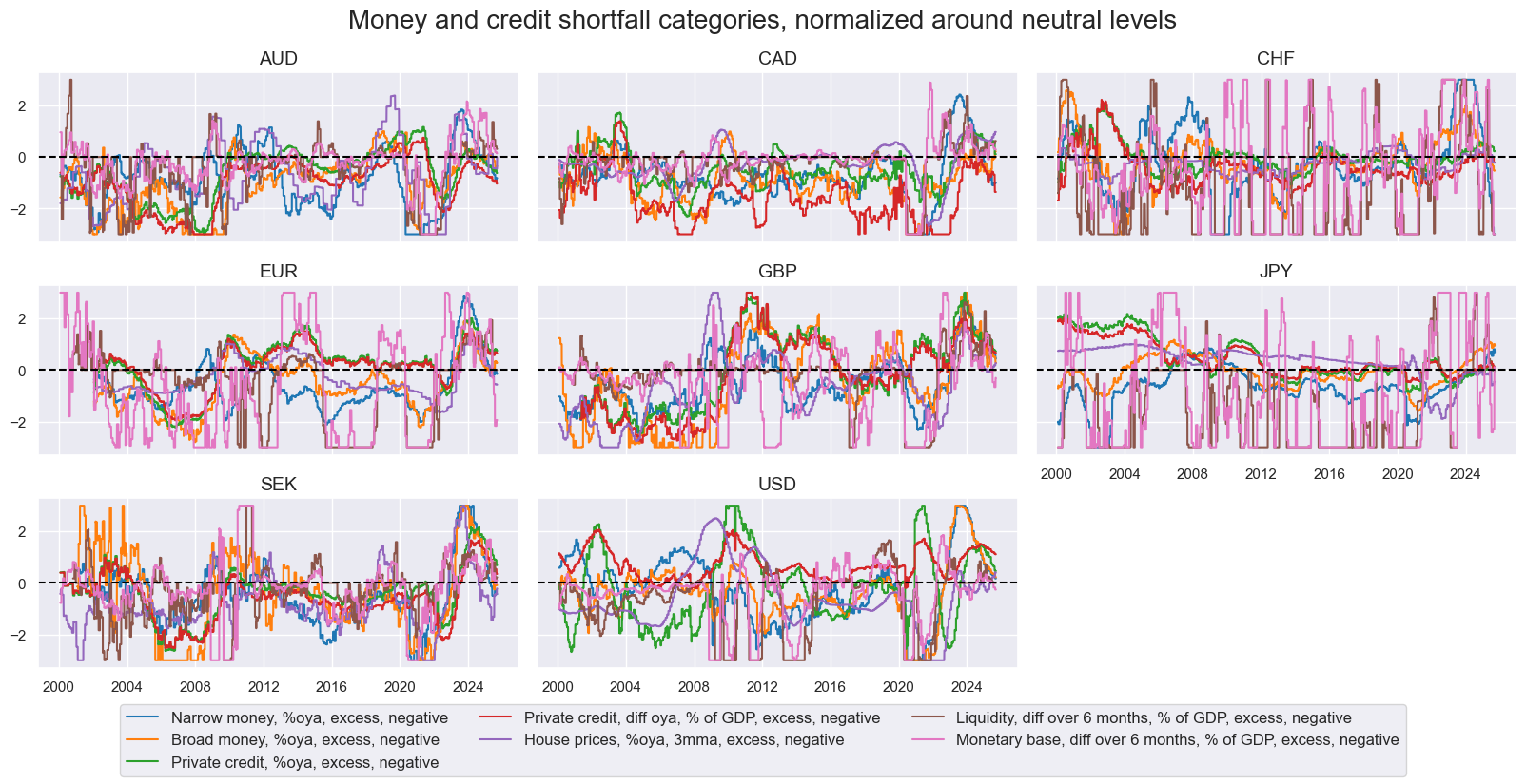
dict_labels["XMNARROW_SJA_P1M1ML12N_ZN"] = "Narrow money, %oya, excess, negative"
dict_labels["XMBROAD_SJA_P1M1ML12N_ZN"] = "Broad money, %oya, excess, negative"
dict_labels["XPCREDITBN_SJA_P1M1ML12N_ZN"] = "Private credit, %oya, excess, negative"
dict_labels["XPCREDITGDP_SJA_D1M1ML12N_ZN"] = "Private credit, diff oya, % of GDP, excess, negative"
dict_labels["XHPI_SA_P1M1ML12_3MMAN_ZN"] = "House prices, %oya, 3mma, excess, negative"
dict_labels["MBASEGDP_SA_D1M1ML6N_ZN"] = "Monetary base, diff over 6 months, % of GDP, excess, negative"
dict_labels["INTLIQGDP_NSA_D1M1ML6N_ZN"] = "Liquidity, diff over 6 months, % of GDP, excess, negative"
# Factors
dict_factorz["XMONNZ"] = [f"{xcat}_ZN" for xcat in xmcr if any(s in xcat for s in mon)]
dict_factorz["XCRHNZ"] = [f"{xcat}_ZN" for xcat in xmcr if any(s in xcat for s in crh)]
dict_factorz["XMCRNZ_BROAD"] = [
f"{xcat}_ZN" for xcat in xmcr if any(s in xcat for s in mcr)
]
factor = "XMCRNZ_BROAD" # XMONNZ, XCRHNZ
xcatx = dict_factorz[factor]
msp.view_timelines(
dfx,
xcats=xcatx,
cids=cids,
ncol=3,
aspect=2,
height=1.8,
start="2000-01-01",
same_y=True,
title="Money and credit shortfall categories, normalized around neutral levels",
title_fontsize=20,
xcat_labels=dict_labels,
)
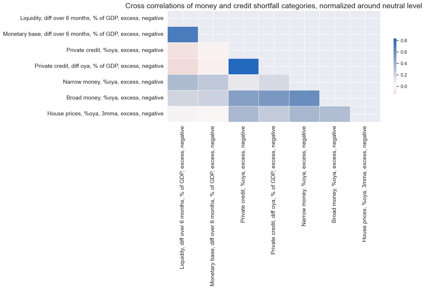
height = len(xcatx)
width = round(height * 1.6)
msp.correl_matrix(
dfx,
xcats=xcatx,
cids=cids,
freq="M",
size=(15, 10),
cluster=True,
title="Cross correlations of money and credit shortfall categories, normalized around neutral level",
title_fontsize=18,
xcat_labels={xcat:dict_labels[xcat] for xcat in xcatx},
)
Equally-weighted conceptual scores #
dfa = pd.DataFrame(columns=dfx.columns)
for k, v in dict_factorz.items():
    dfaa = msp.linear_composite(
        df=dfx,
        xcats=v,
        cids=cids,
        new_xcat=k,
    )
    dfa = msm.update_df(dfa, dfaa)
dfx = msm.update_df(dfx, dfa)

narrow_factorz = [k for k in dict_factorz.keys() if "BROAD" not in k]
broad_factorz = [k for k in dict_factorz.keys() if "BROAD" in k]
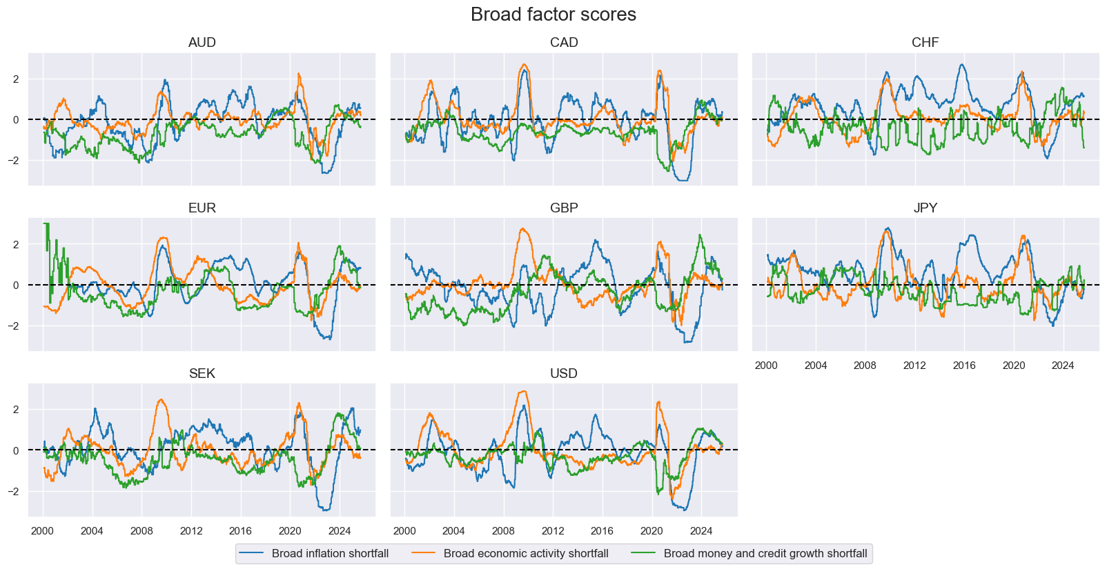
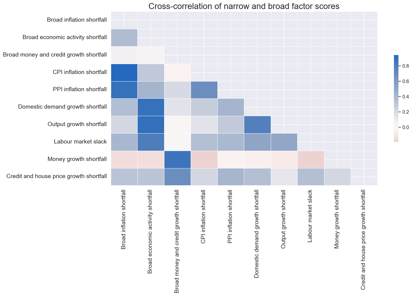
dict_factlabels ={
    "XINFNZ_BROAD": "Broad inflation shortfall",
    "XECGNZ_BROAD": "Broad economic activity shortfall",
    "XMCRNZ_BROAD": "Broad money and credit growth shortfall",
    "XCPINZ": "CPI inflation shortfall",
    "XPPINZ": "PPI inflation shortfall",
    "XDEMNZ": "Domestic demand growth shortfall",
    "XOUTNZ": "Output growth shortfall",
    "XLABNZ": "Labour market slack",
    "XMONNZ": "Money growth shortfall",
    "XCRHNZ": "Credit and house price growth shortfall",
}
dict_labels.update(dict_factlabels)
# Visual check of factor groups

xcatx = broad_factorz  # narrow_factorz broad_factorz

msp.view_timelines(
    dfx,
    xcats=xcatx,
    cids=cids,
    ncol=3,
    aspect=2,
    height=1.8,
    start="2000-01-01",
    same_y=True,
    title="Broad factor scores",
    title_fontsize=20,
    xcat_labels={xcat:dict_labels[xcat] for xcat in xcatx},
)
xcatx = broad_factorz + narrow_factorz

height = len(xcatx)
width = round(height * 1.5)

msp.correl_matrix(
    dfx,
    xcats=xcatx,
    cids=cids,
    freq="M",
    size=(width, height),
    cluster=False,
    title="Cross-correlation of narrow and broad factor scores",
    title_fontsize=20,
    xcat_labels={xcat:dict_labels[xcat] for xcat in xcatx},
)
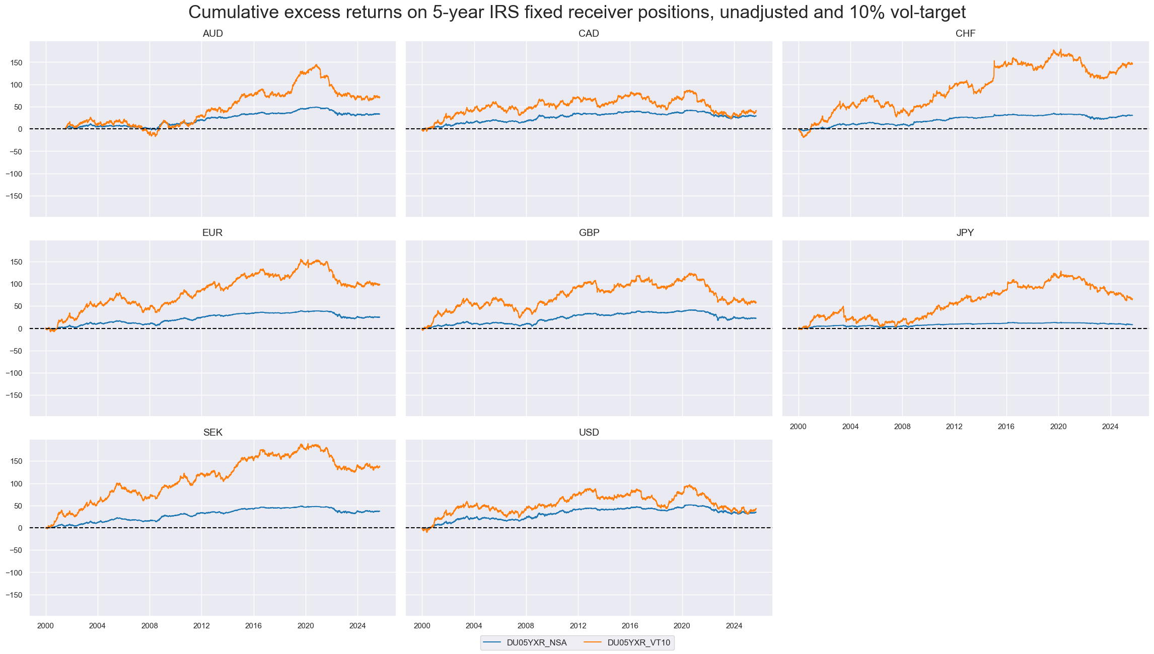
Target returns #
xcatx = ["DU05YXR_NSA", "DU05YXR_VT10"]

msp.view_timelines(
    dfx,
    xcats=xcatx,
    cumsum=True,
    cids=cids,
    ncol=3,
    aspect=1.8,
    start="2000-01-01",
    same_y=True,
    title="Cumulative excess returns on 5-year IRS fixed receiver positions, unadjusted and 10% vol-target",
    title_fontsize=26,
)
Signal generation #
Preparation #
scorer = {"RMSE": make_scorer(root_mean_squared_error, greater_is_better=False)}
splitter = {"Rolling": msl.RollingKFoldPanelSplit(5)}
from sklearn.base import BaseEstimator, TransformerMixin
from sklearn.cross_decomposition import PLSRegression


class PLSTransformer(BaseEstimator, TransformerMixin):
    def __init__(self, n_components=2):
        self.n_components = n_components
        self.model = PLSRegression(n_components=n_components)

    def fit(self, X, y=None):
        # PLS needs y for supervised decomposition
        # If you're fitting inside a preprocessing pipeline, pass y through
        self.model.fit(X, y)
        return self

    def transform(self, X):
        return self.model.transform(X)
from sklearn.base import MetaEstimatorMixin


class DataFrameTransformer(BaseEstimator, TransformerMixin, MetaEstimatorMixin):
    def __init__(self, transformer, column_names=None):
        # Attributes
        self.transformer = transformer
        self.column_names = column_names

    def fit(self, X, y=None):
        # Fit estimator
        self.transformer.fit(X, y)

        return self

    def transform(self, X):
        # Transform the data
        transformation = self.transformer.transform(X)

        if isinstance(transformation, pd.DataFrame):
            return transformation
        else:
            # scikit-learn returns a numpy array, convert it back to DataFrame
            if self.column_names is None:
                columns = [f"Factor_{i}" for i in range(transformation.shape[1])]
            else:
                columns = self.column_names[: transformation.shape[1]]

            return pd.DataFrame(
                data=transformation,
                columns=columns,
                index=X.index,
            )
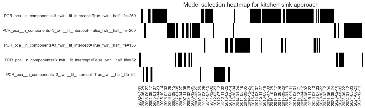
Kitchen-sink PCA and PLS #
xcatx = list(
    itertools.chain(*[dict_factorz[narrow_xcat] for narrow_xcat in narrow_factorz])
) + ["DU05YXR_VT10"]
cidx = cids

so_full = msl.SignalOptimizer(
    df=dfx,
    xcats=xcatx,
    cids=cidx,
    freq="W",
    lag=1,
    xcat_aggs=["last", "sum"],
)
so_full.calculate_predictions(
    name="KS",
    models={
        "PCR": Pipeline(
            [
                ("scaler", msl.PanelStandardScaler()),
                ("pca", msl.PanelPCA(n_components=3)),
                ("twlr", msl.TimeWeightedLinearRegression()),
            ]
        ),
        "PLS": Pipeline(
            [
                ("scaler", msl.PanelStandardScaler()),
                ("pls", DataFrameTransformer(PLSTransformer(n_components=3))),
                ("twlr", msl.TimeWeightedLinearRegression()),
            ]
        ),
    },
    scorers=scorer,
    hyperparameters={
        "PCR": {"twlr__fit_intercept": [True, False], "twlr__half_life": [1*52, 3*52, 5*52], "pca__n_components": [3, 0.95]},
        "PLS": {"twlr__fit_intercept": [True, False], "twlr__half_life": [1*52, 3*52, 5*52], "pls__transformer__n_components": [3, 5]},
    },
    inner_splitters=splitter,
    min_cids=3,
    test_size=4,
    store_correlations=True,
    min_periods=24,
)

so_full.models_heatmap(
    "KS",
    title="Model selection heatmap for kitchen sink approach",
    title_fontsize=18,
    figsize=(12, 4),
)

dfa = so_full.get_optimized_signals("KS")
dfx = msm.update_df(dfx, dfa)
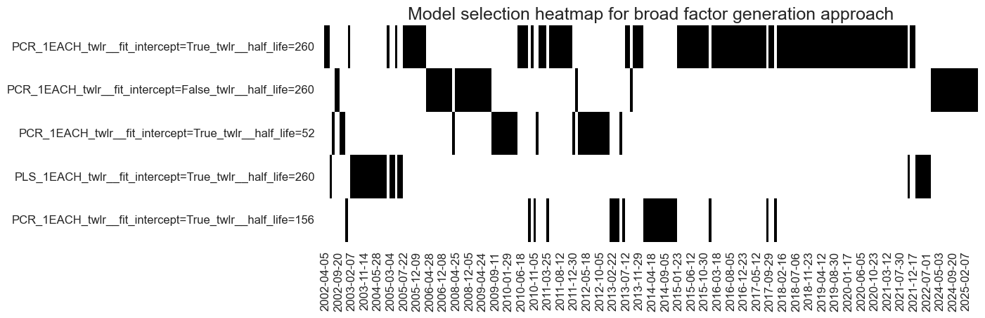
Broad-factor PCA and PLS #
xcatx = list(
    itertools.chain(*[dict_factorz[narrow_xcat] for narrow_xcat in narrow_factorz])
) + ["DU05YXR_VT10"]
cidx = cids

so_broad = msl.SignalOptimizer(
    df=dfx,
    xcats=xcatx,
    cids=cidx,
    freq="W",
    lag=1,
    xcat_aggs=["last", "sum"],
)
so_broad.calculate_predictions(
    name="BROAD",
    models={
        "PCR_1EACH": Pipeline(
            [
                ("scaler", msl.PanelStandardScaler()),
                (
                    "ct",
                    DataFrameTransformer(
                        ColumnTransformer(
                            [
                                (
                                    "pca_inf",
                                    msl.PanelPCA(n_components=1),
                                    dict_factorz["XINFNZ_BROAD"],
                                ),
                                (
                                    "pca_grow",
                                    msl.PanelPCA(n_components=1),
                                    dict_factorz["XECGNZ_BROAD"],
                                ),
                                (
                                    "pca_lend",
                                    msl.PanelPCA(n_components=1),
                                    dict_factorz["XMCRNZ_BROAD"],
                                ),
                            ]
                        ),
                        column_names=["INF", "GROW", "LEND"],
                    ),
                ),
                ("twlr", msl.TimeWeightedLinearRegression()),
            ]
        ),
        "PCR_0.95EACH": Pipeline(
            [
                ("scaler", msl.PanelStandardScaler()),
                (
                    "ct",
                    DataFrameTransformer(
                        ColumnTransformer(
                            [
                                (
                                    "pca_inf",
                                    PCA(n_components=0.95),
                                    dict_factorz["XINFNZ_BROAD"],
                                ),
                                (
                                    "pca_grow",
                                    PCA(n_components=0.95),
                                    dict_factorz["XECGNZ_BROAD"],
                                ),
                                (
                                    "pca_lend",
                                    PCA(n_components=0.95),
                                    dict_factorz["XMCRNZ_BROAD"],
                                ),
                            ]
                        )
                    ),
                ),
                ("twlr", msl.TimeWeightedLinearRegression()),
            ]
        ),
        "PLS_1EACH": Pipeline(
            [
                ("scaler", msl.PanelStandardScaler()),
                (
                    "ct",
                    DataFrameTransformer(
                        ColumnTransformer(
                            [
                                (
                                    "pls_inf",
                                    PLSTransformer(n_components=1),
                                    dict_factorz["XINFNZ_BROAD"],
                                ),
                                (
                                    "pls_grow",
                                    PLSTransformer(n_components=1),
                                    dict_factorz["XECGNZ_BROAD"],
                                ),
                                (
                                    "pls_lend",
                                    PLSTransformer(n_components=1),
                                    dict_factorz["XMCRNZ_BROAD"],
                                ),
                            ]
                        ),
                        column_names=["INF", "GROW", "LEND"],
                    ),
                ),
                ("twlr", msl.TimeWeightedLinearRegression()),
            ]
        ),
    },
    scorers=scorer,
    hyperparameters={
        "PCR_1EACH": {"twlr__fit_intercept": [True, False], "twlr__half_life": [1*52, 3*52, 5*52]},
        "PCR_0.95EACH": {"twlr__fit_intercept": [True, False], "twlr__half_life": [1*52, 3*52, 5*52]},
        "PLS_1EACH": {"twlr__fit_intercept": [True, False], "twlr__half_life": [1*52, 3*52, 5*52]},
    },
    inner_splitters=splitter,
    min_cids=3,
    min_periods=24,
    test_size=4,
)


so_broad.models_heatmap(
    "BROAD",
    title="Model selection heatmap for broad factor generation approach",
    title_fontsize=18,
    figsize=(12, 4),
)

dfa = so_broad.get_optimized_signals("BROAD")
dfx = msm.update_df(dfx, dfa)
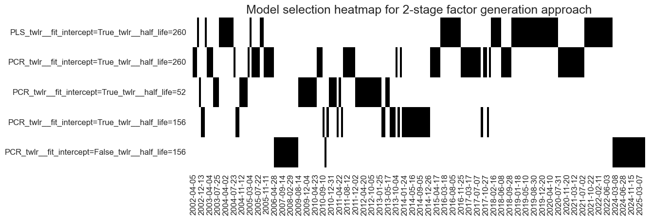
2-stage factor PCA/PLS #
xcatx = list(
    itertools.chain(*[dict_factorz[narrow_xcat] for narrow_xcat in narrow_factorz])
) + ["DU05YXR_VT10"]
cidx = cids

so_narrow = msl.SignalOptimizer(
    df=dfx,
    xcats=xcatx,
    cids=cidx,
    freq="W",
    lag=1,
    xcat_aggs=["last", "sum"],
)
so_narrow.calculate_predictions(
    name="TWOSTAGE",
    models={
        "PCR": Pipeline(
            [
                ("scaler", msl.PanelStandardScaler()),
                (
                    "ct",
                    DataFrameTransformer(
                        transformer=ColumnTransformer(
                            [
                                (
                                    "pca_cpi",
                                    PCA(n_components=1),
                                    dict_factorz["XCPINZ"],
                                ),
                                (
                                    "pca_ppi",
                                    PCA(n_components=1),
                                    dict_factorz["XPPINZ"],
                                ),
                                (
                                    "pca_dem",
                                    PCA(n_components=1),
                                    dict_factorz["XDEMNZ"],
                                ),
                                (
                                    "pca_out",
                                    PCA(n_components=1),
                                    dict_factorz["XOUTNZ"],
                                ),
                                (
                                    "pca_lab",
                                    PCA(n_components=1),
                                    dict_factorz["XLABNZ"],
                                ),
                                (
                                    "pca_mon",
                                    PCA(n_components=1),
                                    dict_factorz["XMONNZ"],
                                ),
                                (
                                    "pca_cre",
                                    PCA(n_components=1),
                                    dict_factorz["XCRHNZ"],
                                ),
                            ]
                        ),
                        column_names=["CPI", "PPI", "DEM", "OUT", "LAB", "MON", "CRE"],
                    ),
                ),
                ("scaler2", msl.PanelStandardScaler()),
                (
                    "ct2",
                    DataFrameTransformer(
                        ColumnTransformer(
                            [
                                ("pca_inf", PCA(n_components=1), ["CPI", "PPI"]),
                                (
                                    "pca_grow",
                                    PCA(n_components=1),
                                    ["DEM", "OUT", "LAB"],
                                ),
                                ("pca_lend", PCA(n_components=1), ["MON", "CRE"]),
                            ]
                        )
                    ),
                ),
                ("twlr", msl.TimeWeightedLinearRegression()),
            ]
        ),
        "PLS": Pipeline(
            [
                ("scaler", msl.PanelStandardScaler()),
                (
                    "ct",
                    DataFrameTransformer(
                        transformer=ColumnTransformer(
                            [
                                (
                                    "pls_cpi",
                                    PLSTransformer(n_components=1),
                                    dict_factorz["XCPINZ"],
                                ),
                                (
                                    "pls_ppi",
                                    PLSTransformer(n_components=1),
                                    dict_factorz["XPPINZ"],
                                ),
                                (
                                    "pls_dem",
                                    PLSTransformer(n_components=1),
                                    dict_factorz["XDEMNZ"],
                                ),
                                (
                                    "pls_out",
                                    PLSTransformer(n_components=1),
                                    dict_factorz["XOUTNZ"],
                                ),
                                (
                                    "pls_lab",
                                    PLSTransformer(n_components=1),
                                    dict_factorz["XLABNZ"],
                                ),
                                (
                                    "pls_mon",
                                    PLSTransformer(n_components=1),
                                    dict_factorz["XMONNZ"],
                                ),
                                (
                                    "pls_cre",
                                    PLSTransformer(n_components=1),
                                    dict_factorz["XCRHNZ"],
                                ),
                            ]
                        ),
                        column_names=["CPI", "PPI", "DEM", "OUT", "LAB", "MON", "CRE"],
                    ),
                ),
                ("scaler2", msl.PanelStandardScaler()),
                (
                    "ct2",
                    DataFrameTransformer(
                        ColumnTransformer(
                            [
                                (
                                    "pls_inf",
                                    PLSTransformer(n_components=1),
                                    ["CPI", "PPI"],
                                ),
                                (
                                    "pls_grow",
                                    PLSTransformer(n_components=1),
                                    ["DEM", "OUT", "LAB"],
                                ),
                                (
                                    "pls_lend",
                                    PLSTransformer(n_components=1),
                                    ["MON", "CRE"],
                                ),
                            ]
                        ),
                    ),
                ),
                ("twlr", msl.TimeWeightedLinearRegression()),
            ]
        ),
    },
    scorers=scorer,
    hyperparameters={
        "PCR": {"twlr__fit_intercept": [True, False], "twlr__half_life": [1*52, 3*52, 5*52]},
        "PLS": {"twlr__fit_intercept": [True, False], "twlr__half_life": [1*52, 3*52, 5*52]},
    },
    inner_splitters=splitter,
    min_cids=3,
    min_periods=24,
    test_size=4,
)


so_narrow.models_heatmap(
    "TWOSTAGE",
    title="Model selection heatmap for 2-stage factor generation approach",
    title_fontsize=18,
    figsize=(12, 4),
)

dfa = so_narrow.get_optimized_signals("TWOSTAGE")
dfx = msm.update_df(dfx, dfa)
Conceptual parity #
dfa = msp.linear_composite(
    df=dfx, xcats=broad_factorz, cids=cids, new_xcat="PARITY"
)

dfx = msm.update_df(dfx, dfa)
Value checks #
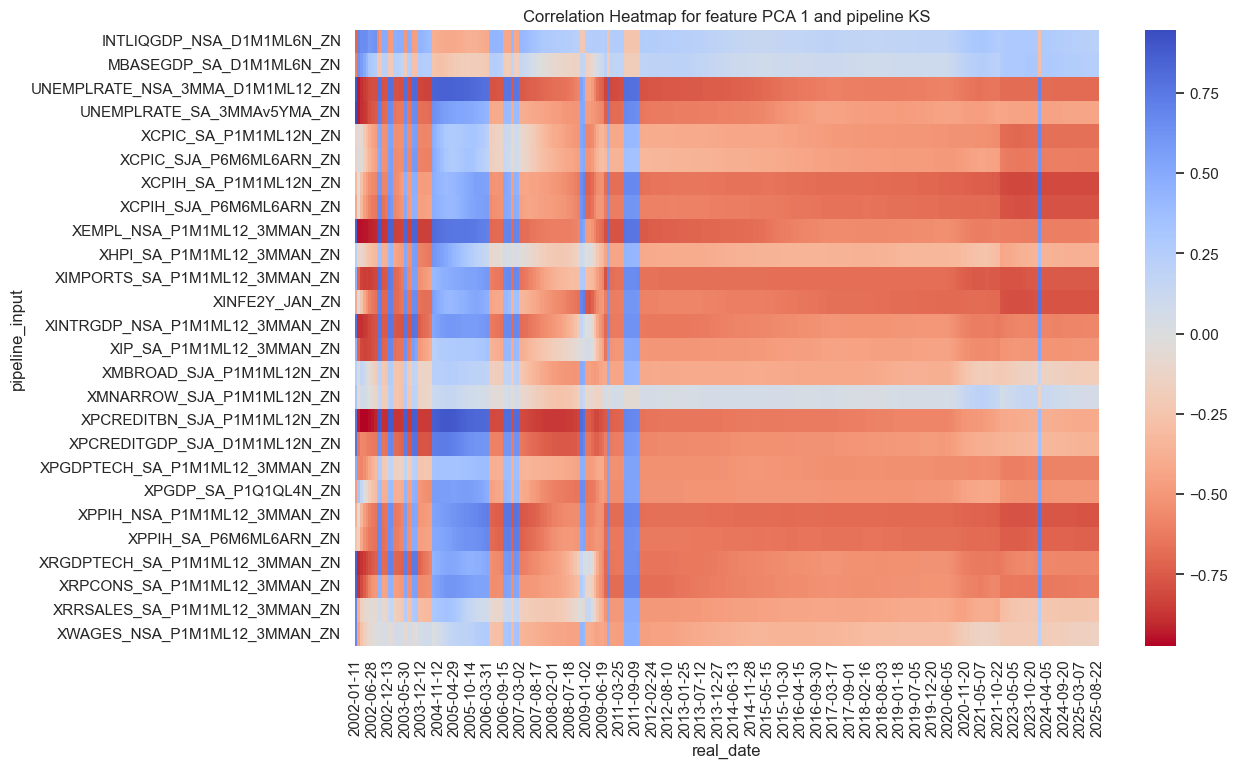
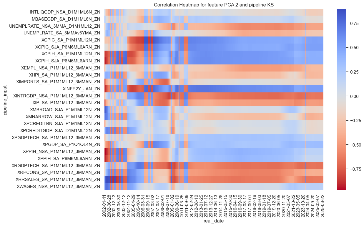
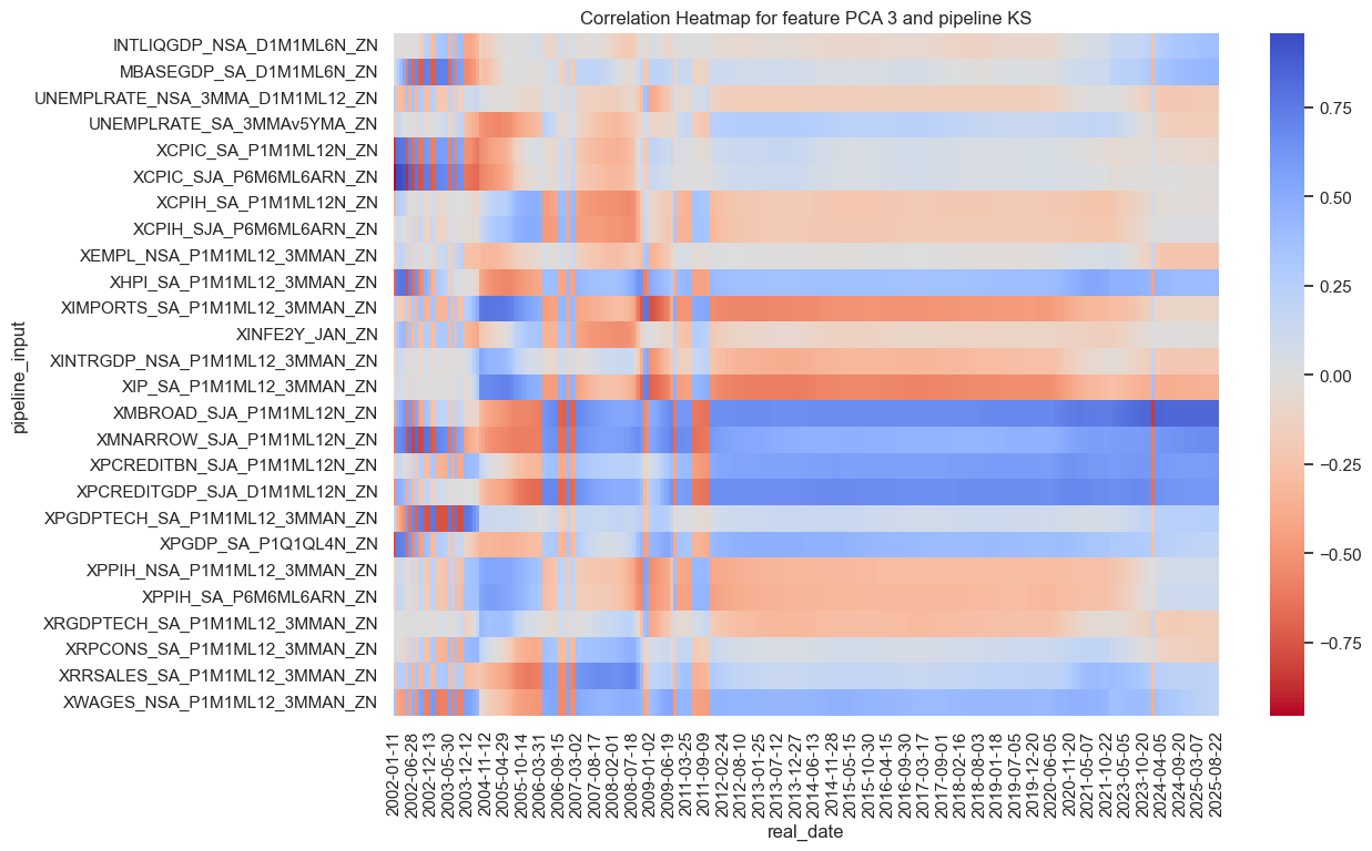
Kitchen-sink component inference #
The kitchen-sink latent factors have converged to inflation, growth and lending factors in order.
so_full.correlations_heatmap(name="KS",feature_name="PCA 1")
so_full.correlations_heatmap(name="KS",feature_name="PCA 2")
so_full.correlations_heatmap(name="KS",feature_name="PCA 3")
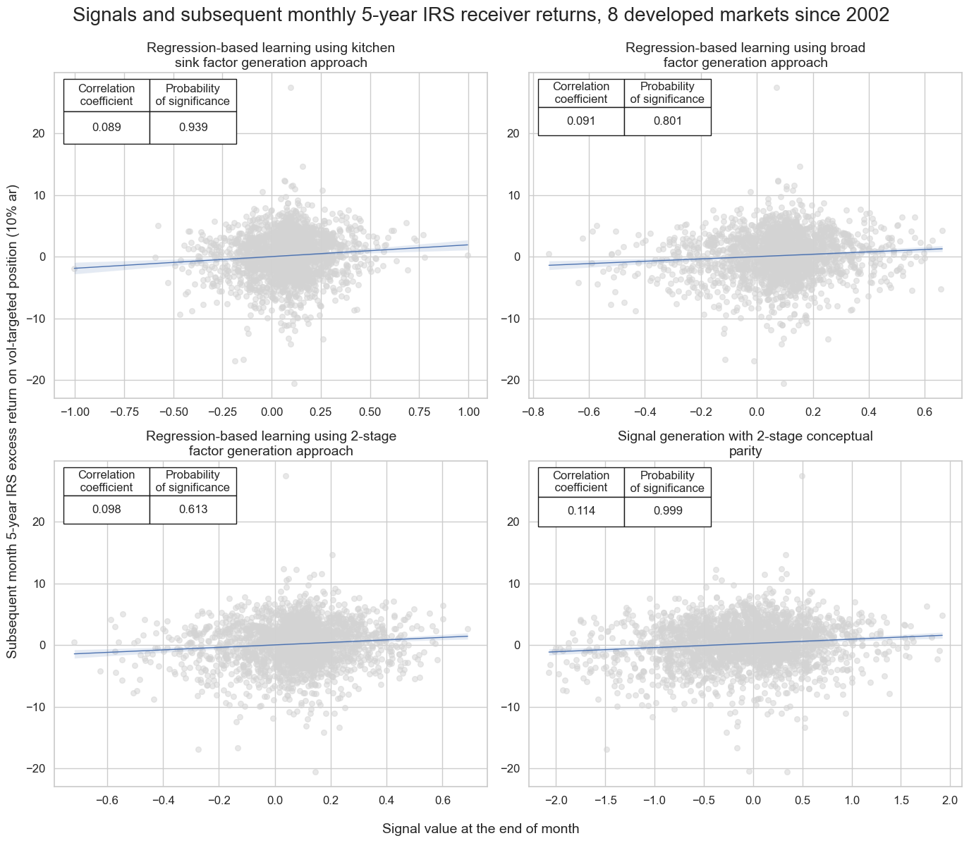
Forward correlation and accuracy #
dict_labels["BROAD"] = "Regression-based learning using broad factor generation approach"
dict_labels["TWOSTAGE"] = "Regression-based learning using 2-stage factor generation approach"
dict_labels["KS"] = "Regression-based learning using kitchen sink factor generation approach"
dict_labels["PARITY"] = "Signal generation with 2-stage conceptual parity"
xcatx = ["KS", "BROAD", "TWOSTAGE", "PARITY"]
titles = [dict_labels[k] for k in xcatx]
crs = []

for xcat in xcatx:
    cr = msp.CategoryRelations(
        df=dfx,
        xcats=[xcat, "DU05YXR_VT10"],
        cids=cids,
        freq="M",
        lag=1,
        xcat_aggs=["last", "sum"],
        slip=1,
        start="2002-01-11",
    )
    crs.append(cr)

msv.multiple_reg_scatter(
    cat_rels=crs,
    ncol=2,
    nrow=2,
    figsize=(14, 12),
    prob_est="map",
    coef_box="upper left",
    title="Signals and subsequent monthly 5-year IRS receiver returns, 8 developed markets since 2002",
    title_fontsize=20,
    subplot_titles=titles,
    xlab="Signal value at the end of month",
    ylab="Subsequent month 5-year IRS excess return on vol-targeted position (10% ar)",
    share_axes=False,
    label_fontsize=14,
)
xcatx = ["KS", "BROAD", "TWOSTAGE", "PARITY"]
dict_short_labels = {}
dict_short_labels["BROAD"] = "Broad factor approach"
dict_short_labels["TWOSTAGE"] = "2-stage factor approach"
dict_short_labels["KS"] = "Kitchen sink approach"
dict_short_labels["PARITY"] = "2-stage conceptual parity"
srr = mss.SignalReturnRelations(
dfx,
cids=cids,
sigs=xcatx,
rets=["DU05YXR_VT10"],
freqs=["M", "W"],
start="2002-02-28",
)
pd.set_option("display.precision", 3)
display(srr.multiple_relations_table().round(3))
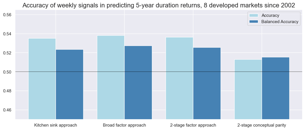
srr.accuracy_bars(
type="signals",
title="Accuracy of weekly signals in predicting 5-year duration returns, 8 developed markets since 2002",
freq="W",
size=(13, 5),
x_labels=dict_short_labels
)
| accuracy | bal_accuracy | pos_sigr | pos_retr | pos_prec | neg_prec | pearson | pearson_pval | kendall | kendall_pval | auc | ||||
|---|---|---|---|---|---|---|---|---|---|---|---|---|---|---|
| Return | Signal | Frequency | Aggregation | |||||||||||
| DU05YXR_VT10 | BROAD | M | last | 0.542 | 0.525 | 0.754 | 0.546 | 0.558 | 0.492 | 0.094 | 0.0 | 0.057 | 0.000 | 0.519 |
| KS | M | last | 0.545 | 0.529 | 0.750 | 0.546 | 0.560 | 0.498 | 0.087 | 0.0 | 0.048 | 0.001 | 0.522 | |
| PARITY | M | last | 0.531 | 0.533 | 0.473 | 0.551 | 0.587 | 0.480 | 0.114 | 0.0 | 0.063 | 0.000 | 0.534 | |
| TWOSTAGE | M | last | 0.536 | 0.519 | 0.732 | 0.546 | 0.556 | 0.483 | 0.093 | 0.0 | 0.049 | 0.001 | 0.515 | |
| BROAD | W | last | 0.538 | 0.527 | 0.758 | 0.535 | 0.548 | 0.507 | 0.049 | 0.0 | 0.033 | 0.000 | 0.520 | |
| KS | W | last | 0.535 | 0.524 | 0.751 | 0.535 | 0.547 | 0.500 | 0.038 | 0.0 | 0.027 | 0.000 | 0.518 | |
| PARITY | W | last | 0.513 | 0.515 | 0.470 | 0.538 | 0.554 | 0.476 | 0.059 | 0.0 | 0.034 | 0.000 | 0.515 | |
| TWOSTAGE | W | last | 0.536 | 0.525 | 0.734 | 0.535 | 0.548 | 0.502 | 0.046 | 0.0 | 0.030 | 0.000 | 0.520 |
Naive PnLs #
xcatx = ["KS", "BROAD", "TWOSTAGE", "PARITY"]

naive_pnl = msn.NaivePnL(
    dfx,
    cids=cids,
    ret="DU05YXR_VT10",
    sigs=xcatx,
    start="2002-02-28",
    bms=["USD_GB10YXR_NSA", "USD_EQXR_NSA"],
)

for sig in xcatx:
    naive_pnl.make_pnl(
        sig,
        sig_neg=False,
        sig_op="zn_score_pan",
        thresh=2,
        rebal_freq="weekly",
        vol_scale=10,
        rebal_slip=1,
        pnl_name=sig,
    )

naive_pnl.plot_pnls(
    title="Cumulative combined naive PnLs for normalized unbiased signals in eight developed markets",
    title_fontsize=18,
    figsize=(14, 8),
    xcat_labels={xcat:dict_labels[xcat] for xcat in xcatx},
    legend_fontsize=14,
)

pd.set_option("display.precision", 2)
naive_pnl.evaluate_pnls(pnl_cats=naive_pnl.pnl_names, label_dict=dict_short_labels).round(2)
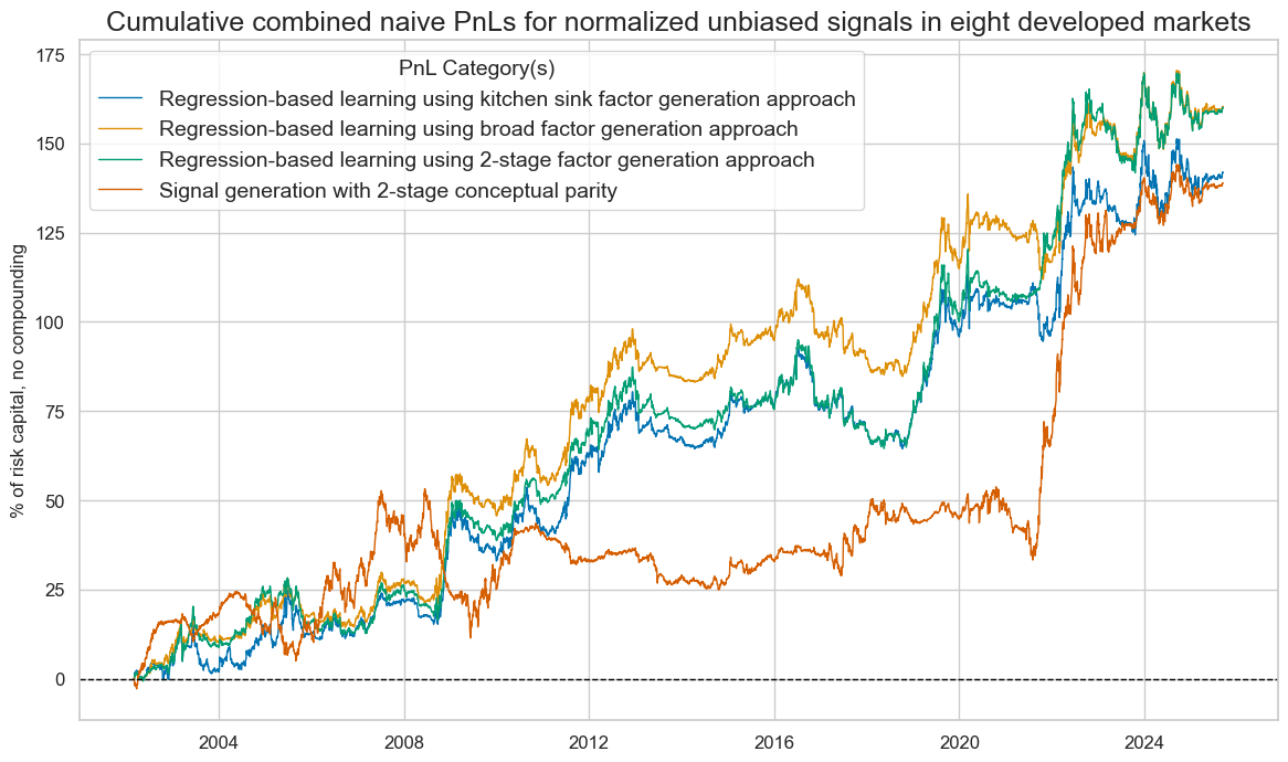
| xcat | Broad factor approach | 2-stage factor approach | Kitchen sink approach | 2-stage conceptual parity |
|---|---|---|---|---|
| Return % | 6.81 | 6.79 | 6.02 | 5.9 |
| St. Dev. % | 10.0 | 10.0 | 10.0 | 10.0 |
| Sharpe Ratio | 0.68 | 0.68 | 0.6 | 0.59 |
| Sortino Ratio | 0.99 | 0.98 | 0.86 | 0.86 |
| Max 21-Day Draw % | -11.58 | -11.38 | -12.26 | -12.43 |
| Max 6-Month Draw % | -17.56 | -18.24 | -18.02 | -26.76 |
| Peak to Trough Draw % | -27.33 | -30.43 | -27.83 | -41.79 |
| Top 5% Monthly PnL Share | 0.84 | 0.89 | 0.93 | 1.09 |
| USD_GB10YXR_NSA correl | 0.4 | 0.36 | 0.38 | -0.1 |
| USD_EQXR_NSA correl | -0.2 | -0.18 | -0.18 | -0.01 |
| Traded Months | 284 | 284 | 284 | 284 |
xcatx = ["KS", "BROAD", "TWOSTAGE", "PARITY"]

naive_pnl = msn.NaivePnL(
    dfx,
    ret="DU05YXR_VT10",
    sigs=xcatx,
    start="2002-02-28",
    bms=["USD_GB10YXR_NSA", "USD_EQXR_NSA"],
)

for sig in xcatx:
    naive_pnl.make_pnl(
        sig,
        sig_neg=False,
        sig_op="zn_score_pan",
        sig_add=1,
        thresh=2,
        rebal_freq="weekly",
        vol_scale=10,
        rebal_slip=1,
        pnl_name=sig,
    )

naive_pnl.plot_pnls(
    title="Cumulative combined naive PnLs for long-biased normalized signals in eight developed markets",
    title_fontsize=18,
    figsize=(14, 8),
    xcat_labels={xcat:dict_labels[xcat] for xcat in xcatx},
    legend_fontsize=14,
)

pd.set_option("display.precision", 2)
naive_pnl.evaluate_pnls(pnl_cats=naive_pnl.pnl_names, label_dict=dict_short_labels).round(2)
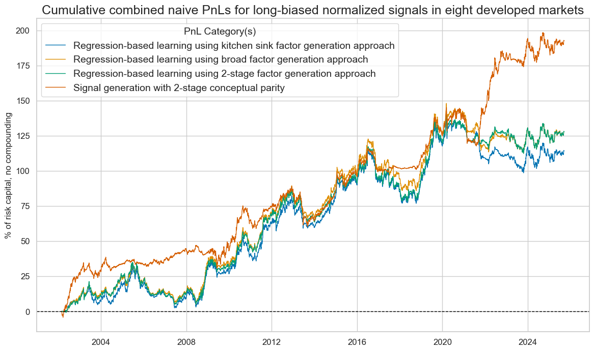
| xcat | Broad factor approach | 2-stage factor approach | Kitchen sink approach | 2-stage conceptual parity |
|---|---|---|---|---|
| Return % | 5.43 | 5.43 | 4.85 | 8.19 |
| St. Dev. % | 10.0 | 10.0 | 10.0 | 10.0 |
| Sharpe Ratio | 0.54 | 0.54 | 0.49 | 0.82 |
| Sortino Ratio | 0.77 | 0.78 | 0.69 | 1.17 |
| Max 21-Day Draw % | -12.82 | -13.7 | -13.0 | -17.88 |
| Max 6-Month Draw % | -21.15 | -22.77 | -21.54 | -25.35 |
| Peak to Trough Draw % | -36.77 | -38.97 | -40.5 | -28.49 |
| Top 5% Monthly PnL Share | 1.0 | 1.0 | 1.12 | 0.69 |
| USD_GB10YXR_NSA correl | 0.6 | 0.59 | 0.6 | 0.37 |
| USD_EQXR_NSA correl | -0.22 | -0.21 | -0.21 | -0.16 |
| Traded Months | 284 | 284 | 284 | 284 |