Introduction to the Macrosynergy package

This notebook shows how the macrosynergy package streamlines working with JPMaQS data. For more detail on the JPMaQS setup, see this notebook .

It begins with an overview of obtaining and describing the data, including tools for exploring availability, distributions, and time series. The next section focuses on preprocessing , showing how to filter, transform, and standardize data, as well as create indicators. Following this, the relating section highlights methods for investigating relationships across different panels, including correlation analysis and regression-based exploration. The final section, signaling , illustrates how to assess the predictive power of signals in relation to returns.

Together, these steps provide a practical workflow for systematic data analysis using the Macrosynergy package.

Get packages and JPMaQS data

# Uncomment to update the package
"""
%%capture
! pip install macrosynergy --upgrade"""

import numpy as np
import pandas as pd
import matplotlib.pyplot as plt
import seaborn as sns
import os

import macrosynergy.management as msm 
import macrosynergy.panel as msp
import macrosynergy.signal as mss
import macrosynergy.pnl as msn
import macrosynergy.visuals as msv
import macrosynergy.learning as msl

from macrosynergy.download import JPMaQSDownload

# machine learning modules
from sklearn.pipeline import Pipeline
from sklearn.linear_model import LogisticRegression, LinearRegression, Ridge
from sklearn.neighbors import KNeighborsClassifier, KNeighborsRegressor

from sklearn.metrics import (make_scorer, balanced_accuracy_score,r2_score,)

import warnings
warnings.simplefilter("ignore")

The JPMaQSDownload() function connects to the JPMaQS DataQuery API and downloads macro-financial data for analysis.

See the JPMaQS Intro Notebook for full details.

Important details:

• client_id : Your API client identifier.

• client_secret : Secret used to authenticate.

• oauth : When True , enables OAuth flow for secure token retrieval.

Note that client_id and client_secret are recommended to be stored as environment variables for security.

cids_dm = ["AUD", "CAD", "CHF", "EUR", "GBP", "JPY", "NOK", "NZD", "SEK", "USD"]
cids_em = ["CLP","COP", "CZK", "HUF", "IDR", "ILS", "INR", "KRW", "MXN", "PLN", "THB", "TRY", "TWD", "ZAR",]
cids = cids_dm + cids_em

cids_dux = list(set(cids) - set(["IDR", "NZD"]))

ecos = [
    # Inflation
    "CPIC_SA_P1M1ML12",
    "CPIC_SJA_P3M3ML3AR",
    "CPIC_SJA_P6M6ML6AR",
    "CPIH_SA_P1M1ML12",
    "CPIH_SJA_P3M3ML3AR",
    "CPIH_SJA_P6M6ML6AR",
    # Nominal and real yields
    "RYLDIRS02Y_NSA",
    "RYLDIRS05Y_NSA",
    "INFTEFF_NSA",
    # GDP
    "RGDP_SA_P1Q1QL4_20QMA",
    "INTRGDP_NSA_P1M1ML12_3MMA",
    "INTRGDPv5Y_NSA_P1M1ML12_3MMA",
    # Private credit
    "PCREDITGDP_SJA_D1M1ML12",
    "PCREDITBN_SJA_P1M1ML12",
]
mkts = [
    # Duration returns
    "DU02YXR_NSA",
    "DU05YXR_NSA",
    "DU02YXR_VT10",
    "DU05YXR_VT10",
    # Equity returns
    "EQXR_NSA",
    "EQXR_VT10",
    # FX
    "FXXR_NSA",
    "FXXR_VT10",
    "FXCRR_NSA",
    "FXTARGETED_NSA",
    "FXUNTRADABLE_NSA",
]

xcats = ecos + mkts

# Download series from J.P. Morgan DataQuery by tickers
start_date = "2000-01-01"
end_date = "2023-05-01"

tickers = [cid + "_" + xcat for cid in cids for xcat in xcats]
print(f"Maximum number of tickers is {len(tickers)}") 
        

# Download series from J.P. Morgan DataQuery by tickers
client_id: str = os.getenv("DQ_CLIENT_ID")
client_secret: str = os.getenv("DQ_CLIENT_SECRET")

with JPMaQSDownload(client_id=client_id, client_secret=client_secret) as dq:
    df = dq.download(
        tickers=tickers,
        start_date="2000-01-01",
        suppress_warning=True,
          show_progress=True,
          metrics='all'
    )

Maximum number of tickers is 600
Downloading data from JPMaQS.
Timestamp UTC:  2025-09-01 11:31:45
Connection successful!

Requesting data: 100%|██████████| 150/150 [00:30<00:00,  4.88it/s]
Downloading data: 100%|██████████| 150/150 [00:49<00:00,  3.01it/s]

Some expressions are missing from the downloaded data. Check logger output for complete list.
105 out of 3000 expressions are missing. To download the catalogue of all available expressions and filter the unavailable expressions, set `get_catalogue=True` in the call to `JPMaQSDownload.download()`.

The Macrosynergy package works with data frames of a standard JPMaQS format. These are long-form DataFrames.

They must include at least four columns:

• cid : cross-section identifier

• xcat : extended category

• real_date : real-time date

• value : data value

#  uncomment if running on Kaggle
"""for dirname, _, filenames in os.walk('/kaggle/input'):
    for filename in filenames:
        print(os.path.join(dirname, filename))
                                                   
df = pd.read_csv('../input/fixed-income-returns-and-macro-trends/JPMaQS_Quantamental_Indicators.csv', index_col=0, parse_dates=['real_date'])""";

The description of each JPMaQS category is available either under Macro Quantamental Academy , JPMorgan Markets (password protected), or on Kaggle (just for the tickers used in this notebook).

df['ticker'] = df['cid'] + "_" + df["xcat"]

dfx = df.copy()
dfx.info() 
dfx.head(3)

<class 'pandas.core.frame.DataFrame'>
RangeIndex: 3649147 entries, 0 to 3649146
Data columns (total 9 columns):
 #   Column        Dtype         
---  ------        -----         
 0   real_date     datetime64[ns]
 1   cid           object        
 2   xcat          object        
 3   value         float64       
 4   grading       float64       
 5   eop_lag       float64       
 6   mop_lag       float64       
 7   last_updated  datetime64[ns]
 8   ticker        object        
dtypes: datetime64[ns](2), float64(4), object(3)
memory usage: 250.6+ MB

	real_date	cid	xcat	value	grading	eop_lag	mop_lag	last_updated	ticker
0	2000-01-03	AUD	CPIC_SJA_P3M3ML3AR	3.006383	2.0	95.0	186.0	2023-01-13 01:03:23	AUD_CPIC_SJA_P3M3ML3AR
1	2000-01-04	AUD	CPIC_SJA_P3M3ML3AR	3.006383	2.0	96.0	187.0	2023-01-13 01:03:23	AUD_CPIC_SJA_P3M3ML3AR
2	2000-01-05	AUD	CPIC_SJA_P3M3ML3AR	3.006383	2.0	97.0	188.0	2023-01-13 01:03:23	AUD_CPIC_SJA_P3M3ML3AR

Describing

View available data history with check_availability and missing_in_df

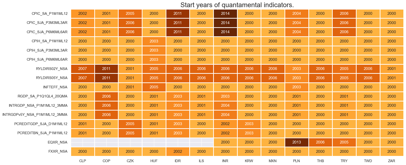
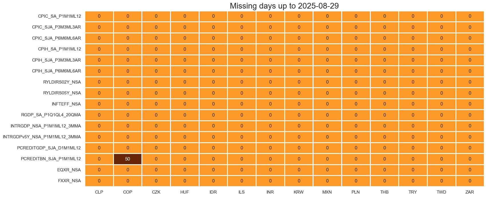
The check_availability() function summarizes data availability across time, categories, and countries or markets (cross-sections). It shows unavailable series and uses color intensity to indicate the starting year of available data (darker = more recent).

This is useful as a quick data coverage check before building anything.

Important parameters include:

• df : Your JPMaQS-standard DataFrame containing the research dataset.

• xcats : A list of signal names to check (e.g., “FX carry”, “Real yield”).

• cids : A list of cross-sections (e.g., “USD”, “EUR”, “JPY”) to evaluate.

• start : Earliest date to consider.

• missing_recent : If True , displays missing data in the most recent period.

msm.check_availability(
    dfx,
    xcats=ecos + ["EQXR_NSA"]+ ["FXXR_NSA"],
    cids=cids_em,
    start="2000-01-01",
    title_fontsize=20
)

The missing_in_df() function lists categories entirely missing across all selected cross-sections and specific cross-sections that are missing for each selected category.

This saves you from having to spot mistakes due to ‘NAs’ later.

cats_exp = ["EQCRR_NSA", "FXCRR_NSA", "INTRGDP_NSA_P1M1ML12_3MMA", "RUBBISH"]
msm.missing_in_df(dfx, xcats=cats_exp, cids=cids)

Missing XCATs across DataFrame:  ['RUBBISH', 'EQCRR_NSA']
Missing cids for FXCRR_NSA:                  ['USD']
Missing cids for INTRGDP_NSA_P1M1ML12_3MMA:  []

Visualize Panel Distributions and Time Series with view_ranges and view_timelines

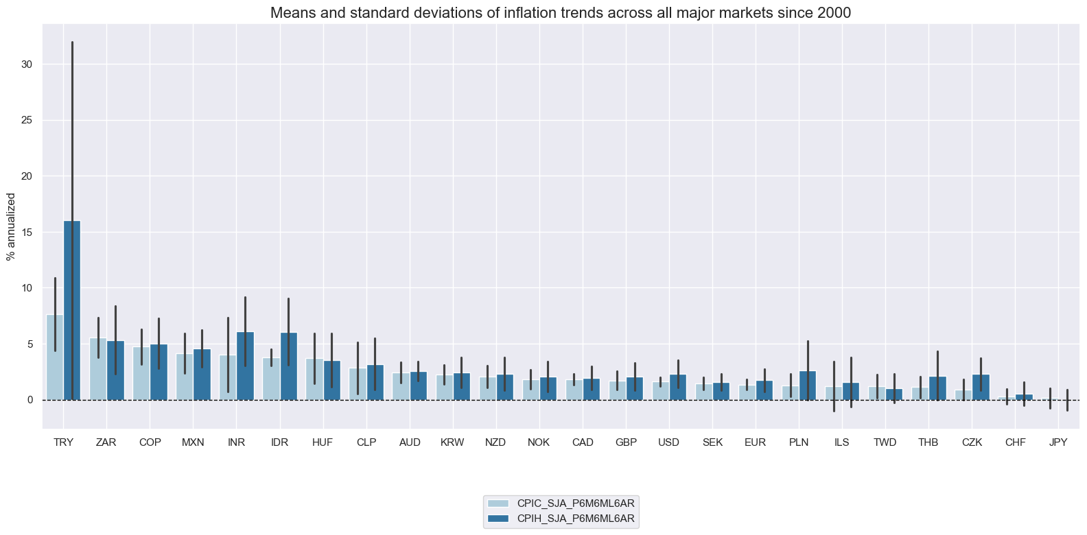
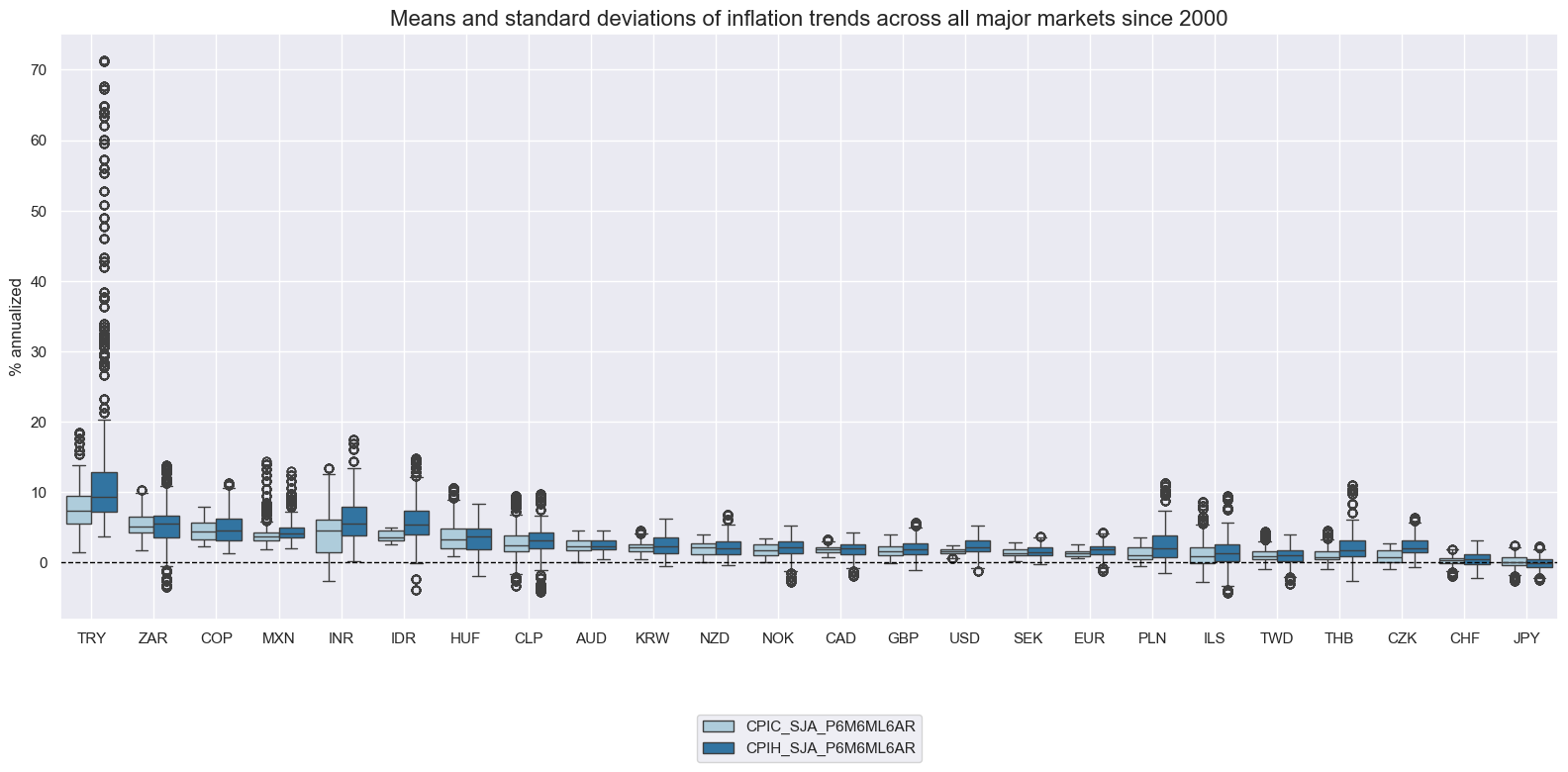
The view_ranges() function compares data ranges across cross-sections or categories.

The function is ideal for comparing scale and volatility.

Important parameters include:

• start and end : Date window.

• kind : Plot type:

  • bar for a barplot that focuses on means and standard deviations of one or more categories across sections for a given sample period; and

xcats_sel = ["CPIC_SJA_P6M6ML6AR", "CPIH_SJA_P6M6ML6AR"]
msp.view_ranges(
    dfx,
    xcats=xcats_sel,
    kind="bar", 
    sort_cids_by="mean",  # Countries sorted by mean of the first category
    title="Means and standard deviations of inflation trends across all major markets since 2000",
    ylab="% annualized",
    start="2000-01-01",
    end="2020-01-01",
    title_fontsize=20
)

• box for visualizaion of 25%, 50% (median), and 75% quantiles and outliers beyond a normal range.

xcats_sel = ["CPIC_SJA_P6M6ML6AR", "CPIH_SJA_P6M6ML6AR"]
msp.view_ranges(
    dfx,
    xcats=xcats_sel,
    kind="box",
    sort_cids_by="mean",  # Countries sorted by mean of the first category
    title="Means and standard deviations of inflation trends across all major markets since 2000",
    ylab="% annualized",
    start="2000-01-01",
    end="2020-01-01",
    title_fontsize=20
)

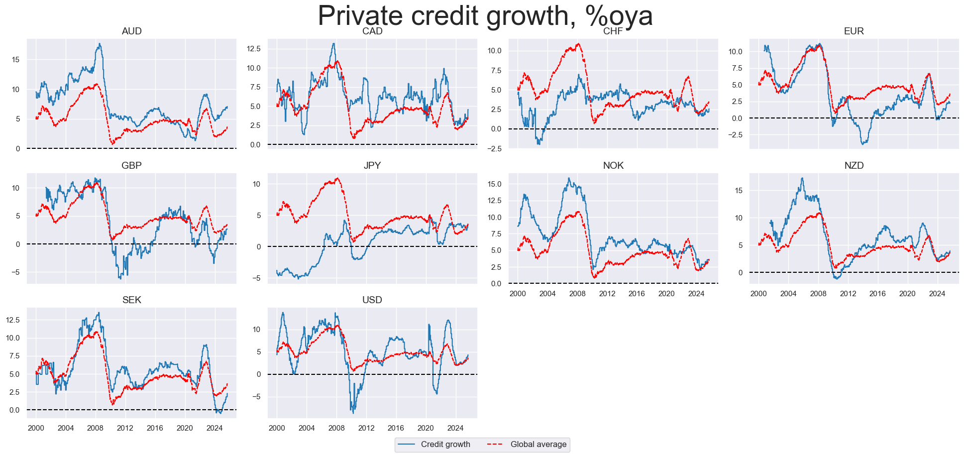
The view_timelines() function visualizes time series data as line charts across multiple cross-sections or categories.

Important parameters include:

• cumsum : When True , plots the cumulative sum of the signal over time instead of raw values. This is useful for return-type or flow-type indicators where you want to track performance or net change over a period.

• same_y : When True , all charts in the grid share the same y-axis scale, making comparison easier.

• blacklist : A dictionary specifying date ranges to exclude for certain assets (e.g. due to data quality issues). Ensures that unreliable data doesn’t distort visual analysis or backtests.

• cs_mean : When True , adds a cross-sectional average line to each plot, letting you quickly compare each asset to the market mean.

msp.view_timelines(
    dfx,
    xcats=["PCREDITBN_SJA_P1M1ML12"],
    cids=cids_dm,
    ncol=4,
    start="1995-01-01",
    title="Private credit growth, %oya",
    same_y=False,
    cs_mean=True,
    xcat_labels=["Credit growth", "Global average"],
     height=2,  # this argument implicitly controls the size of plots relative to labels
    title_fontsize=40
)

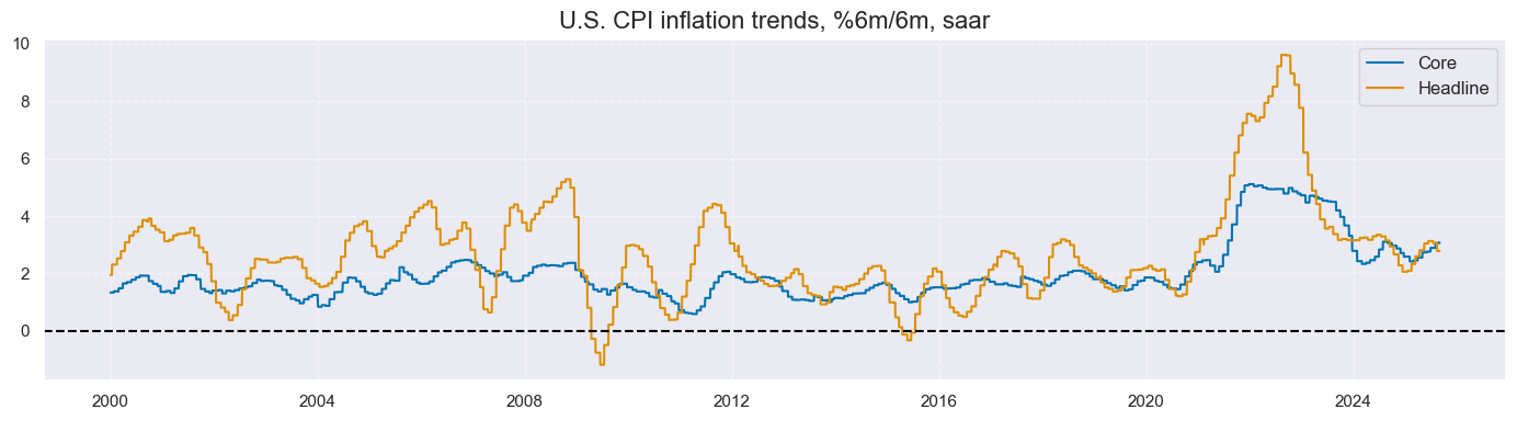
One can display a single chart, displaying several categories for a single cross-section by passing a single-string list to xcats and specifying a cross-section as a list with single element, such as cids=["USD"]

msp.view_timelines(
    dfx,
    xcats=["CPIC_SJA_P6M6ML6AR", "CPIH_SJA_P6M6ML6AR"],
    cids=["USD"],
    start="2000-01-01",
    title="U.S. CPI inflation trends, %6m/6m, saar",
    xcat_labels=["Core", "Headline"],
    size = (14, 4),
    title_fontsize=16
)  

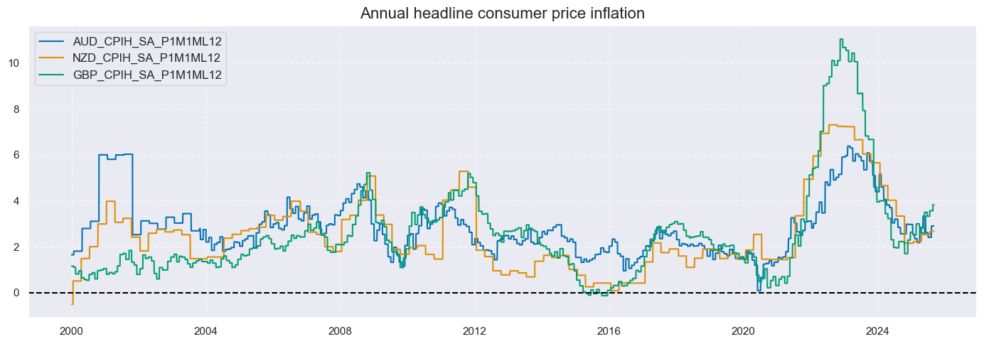
Setting single_chart=True allows plotting a single category for various cross-sections in one plot. Per default, full tickers are used as labels.

cidsx = ["AUD", "NZD", "GBP"]

msp.view_timelines(
    dfx,
    xcats=["CPIH_SA_P1M1ML12"],
    cids=cidsx,
    cumsum=False,
    start="2000-01-01",
    same_y=False,
    title="Annual headline consumer price inflation",
    single_chart=True,
    size = (14, 5),
    title_fontsize=16  
)

Pre-processing

Exclude series sections with make_blacklist and reduce_df

The make_blacklist() function converts binary values in a DataFrame into a summary dictionary of blacklisted time periods. When applied to the blacklist argument of some package functions those cross-sections are excluded from analysis.

Generally, values of 1 in the original binary series are blacklisted.

• nan_black : If True , the function also treats missing values (NaNs) as blacklisted periods.

Below, we selected two indicators of FX tradability and flexibility:

• FXTARGETED_NSA is a dummy variable that equals 1 when the exchange rate is targeted, through a peg or another regime that materially limits flexibility; and 0 otherwise.

• FXUNTRADABLE_NSA is a dummy variable that equals 1 when liquidity in the main FX forward market is restricted or when distortions arise between tradable offshore and untradable onshore contracts.

If one cross section has multiple blacklist periods, the keys are numbered.

# Combine FX tradability and targeting flags into a unified blacklist
dfb = df[df["xcat"].isin(["FXTARGETED_NSA", "FXUNTRADABLE_NSA"])][
    ["cid", "xcat", "real_date", "value"]
]

# Take max value across indicators per date to flag invalid periods (1 if either condition is true)
dfba = (
    dfb.groupby(["cid", "real_date"])
    .agg(value=pd.NamedAgg(column="value", aggfunc="max"))
    .reset_index()
)

dfba["xcat"] = "FXBLACK"
fxblack = msp.make_blacklist(dfba, "FXBLACK")
fxblack

{'CHF': (Timestamp('2011-10-03 00:00:00'), Timestamp('2015-01-30 00:00:00')),
 'CZK': (Timestamp('2014-01-01 00:00:00'), Timestamp('2017-07-31 00:00:00')),
 'ILS': (Timestamp('2000-01-03 00:00:00'), Timestamp('2005-12-30 00:00:00')),
 'INR': (Timestamp('2000-01-03 00:00:00'), Timestamp('2004-12-31 00:00:00')),
 'THB': (Timestamp('2007-01-01 00:00:00'), Timestamp('2008-11-28 00:00:00')),
 'TRY_1': (Timestamp('2000-01-03 00:00:00'), Timestamp('2003-09-30 00:00:00')),
 'TRY_2': (Timestamp('2020-01-01 00:00:00'), Timestamp('2024-07-31 00:00:00'))}

The resulting blacklist dictionary can be passed to various package functions to automatically exclude affected periods from analysis. To filter a DataFrame independently of specific functions, use the reduce_df() helper.

# Apply blacklist to remove invalid FX return periods
dffx = df[df["xcat"] == "FXXR_NSA"]
print("Original shape:", dffx.shape)

dffxx = msm.reduce_df(dffx, blacklist=fxblack)
print("Shape after applying blacklist:", dffxx.shape)

Original shape: (153348, 9)
Shape after applying blacklist: (146001, 9)

Custom calculated panels with panel_calculator and update_df

The panel_calculator function transforms data across all cross-sections in a panel.

It is most useful for quickly creating new data panels using formulas, in a way that is easy to repeat and share.

Formulas are expressed as strings, where capitalized category names act as wide dataframes in Python. In this setup, a category such as "OLDCAT" represents a dataframe with time periods as rows and cross-sections as columns. Any operation you could normally perform on such a dataframe in Python can also be written directly into the formula string.

The calcs parameter collects the list of formulas.

When writing these formulas, panel category names not at the beginning or end of the string must always have a space before and after the name. Calculated category and panel operations must be separated by ‘=’.

Examples:

• “NEWCAT = ( OLDCAT1 + 0.5) * OLDCAT2”

• “NEWCAT = np.log( OLDCAT1 ) - np.abs( OLDCAT2 ) ** 1/2”

Following on, update_df integrates the panels back into your main dataset.

Important parameters are:

• df_add : the new DataFrame you want to add.

• xcat_replace : If True , replace overlapping values for listed categories using df_add .

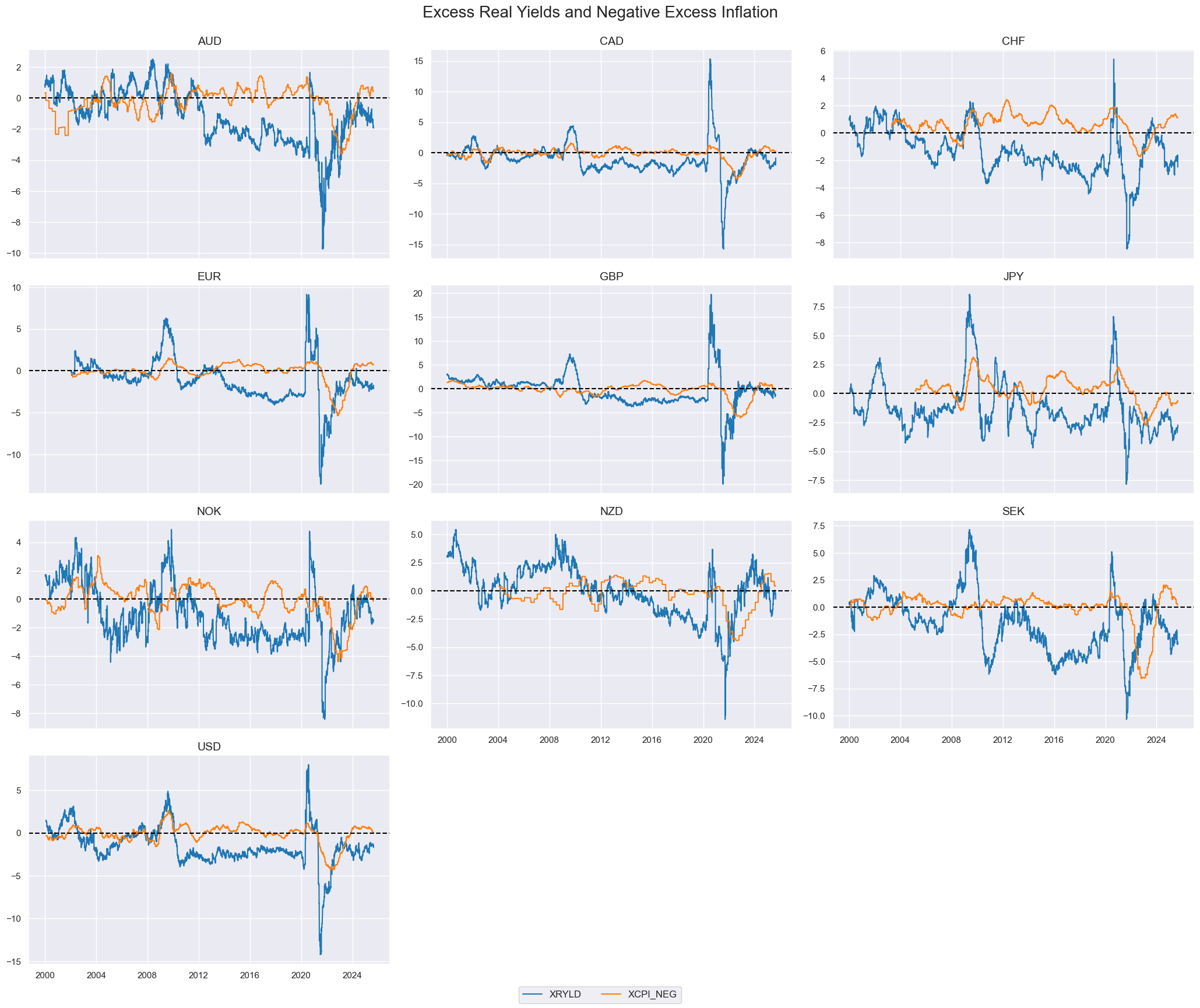
# Define custom panels
calcs = [
    "XGDP_NEG = - INTRGDPv5Y_NSA_P1M1ML12_3MMA",  # negative GDP trend
    "XCPI_NEG = - ( CPIC_SJA_P6M6ML6AR + CPIH_SA_P1M1ML12 ) / 2 + INFTEFF_NSA",  # excess inflation
    "XPCG_NEG = - PCREDITBN_SJA_P1M1ML12 + INFTEFF_NSA + RGDP_SA_P1Q1QL4_20QMA",  # excess credit growth
    "XRYLD = RYLDIRS05Y_NSA - INTRGDP_NSA_P1M1ML12_3MMA",  # excess real yield
    "XXRYLD = XRYLD + XCPI_NEG"  # combined signal
]

# Calculate and merge
dfa = msp.panel_calculator(dfx, calcs=calcs, cids=cids)
dfx = msm.update_df(dfx, dfa)

# Visualization
msp.view_timelines(
    dfx, 
    xcats=["XRYLD", "XCPI_NEG"], 
    cids=cids_dm, 
    ncol=3,
    title="Excess Real Yields and Negative Excess Inflation", 
    start="2000-01-01", 
    same_y=False,
    title_fontsize=20
)

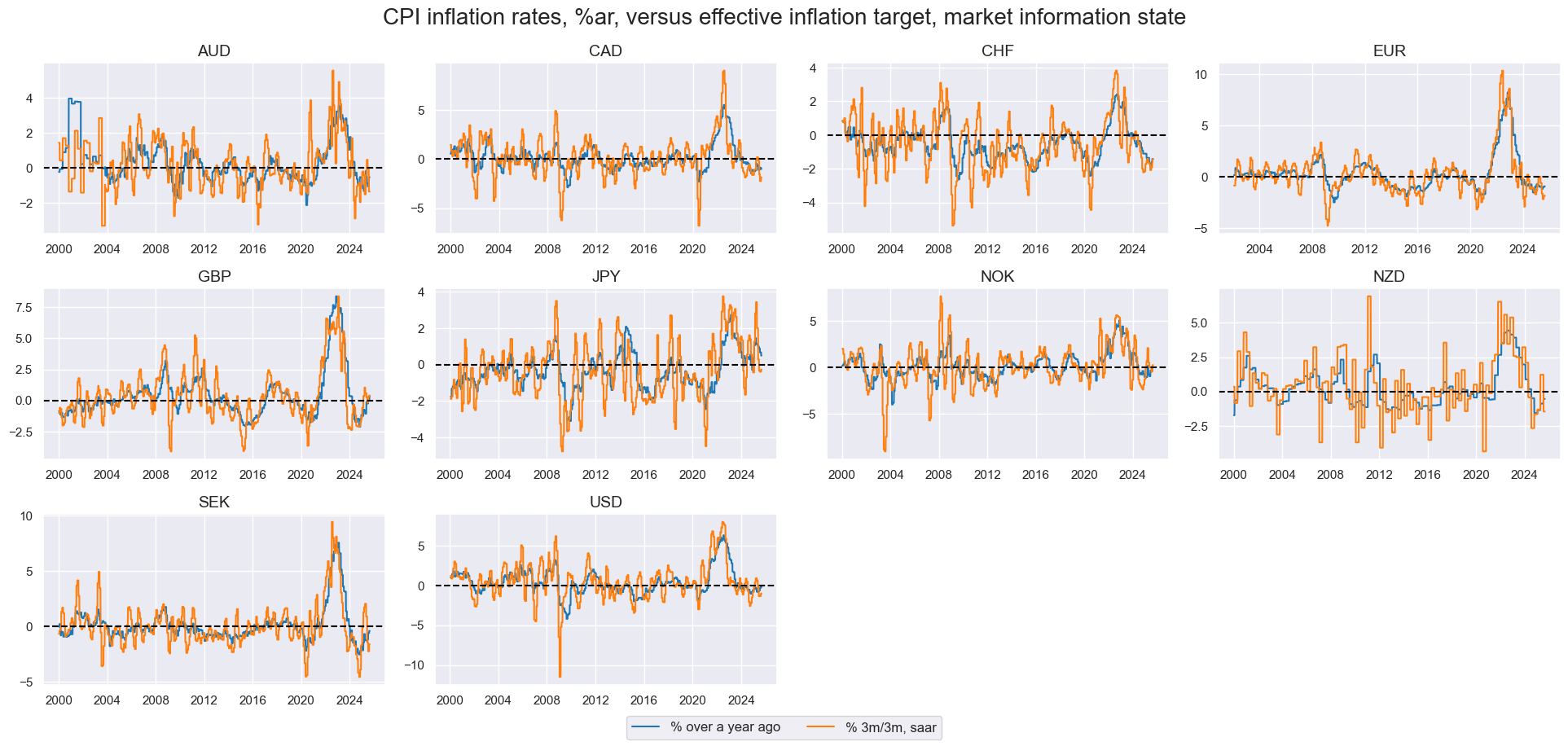
Multiple transformations can be conveniently created using list comprehensions or other string-based iterations.

infs = ["CPIH_SA_P1M1ML12", "CPIH_SJA_P6M6ML6AR", "CPIH_SJA_P3M3ML3AR"]

calcs = [f"{inf}vIET = ( {inf} - INFTEFF_NSA )" for inf in infs]

dfa = msp.panel_calculator(dfx, calcs=calcs, cids=cids)
dfx = msm.update_df(dfx, dfa)


xcatxl = ["CPIH_SA_P1M1ML12vIET", "CPIH_SJA_P3M3ML3ARvIET"]

msp.view_timelines(
    dfx,
    xcats=xcatxl,
    cids=cids_dm,
    ncol=4,
    cumsum=False,
    start="2000-01-01",
    same_y=False,
    all_xticks=True,
    title="CPI inflation rates, %ar, versus effective inflation target, market information state",
    xcat_labels=["% over a year ago", "% 3m/3m, saar"],
    height=2,
    title_fontsize=20
)

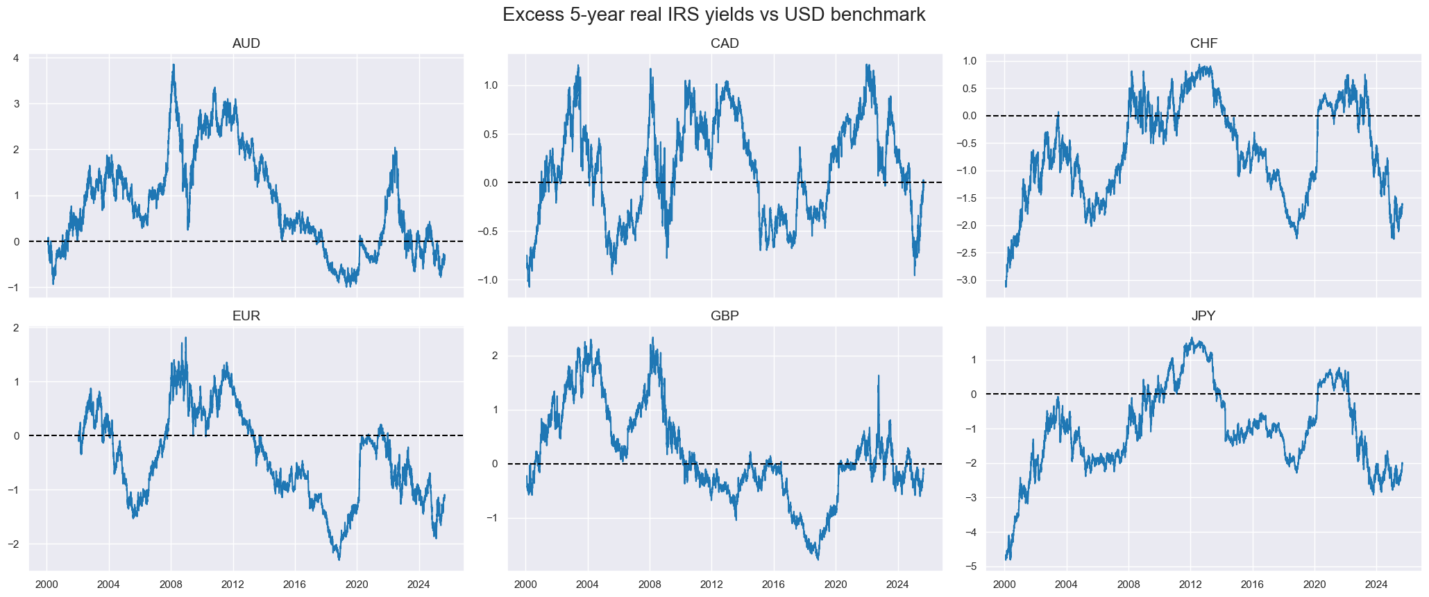
To use a single quantamental indicator instead of a full panel, prefix the category name with "i" followed by the cross-section identifier.

This tells the panel_calculator function to treat the input as a specific cross-section rather than the entire panel.

cidx = cids_dm[:6]
calcs = ["RYLDvUSD = RYLDIRS05Y_NSA -  iUSD_RYLDIRS05Y_NSA"]

dfa = msp.panel_calculator(dfx, calcs=calcs, cids=cidx)
dfx = msm.update_df(dfx, dfa)

msp.view_timelines(
    dfx,
    xcats=["RYLDvUSD"],
    cids=cidx,
    ncol=3,
    start="2000-01-01",
    same_y=False,
    title = "Excess 5-year real IRS yields vs USD benchmark",
    title_fontsize=20

)

Compute panels versus basket with make_relative_value

The make_relative_value() function calculates relative signal values in relation to a cross-sectional benchmark at each date. This can done be through subtraction or division.

Important parameters include:

• rel_meth : The method for making the signal relative, i.e. 'subtract' (default) or 'divide' .

• rel_reference : The benchmark you compare against, i.e 'mean' (default) or 'median' .

• complete_cross : If True , requires all cross-sections to be present on a date and if not, the category is excluded.

• basket : Specifies which cross-sections to use as the relative value benchmark. By default, all cross-sections listed in cids and available in the DataFrame for the given time period are included. However, the benchmark can also be restricted to a valid subset of these cross-sections.

• blacklist : cross-sections and date ranges to exclude, typically created with make_blacklist() . Removing invalid or distorted data is essential, since distortions in just one cross-section can bias all relative value calculations.

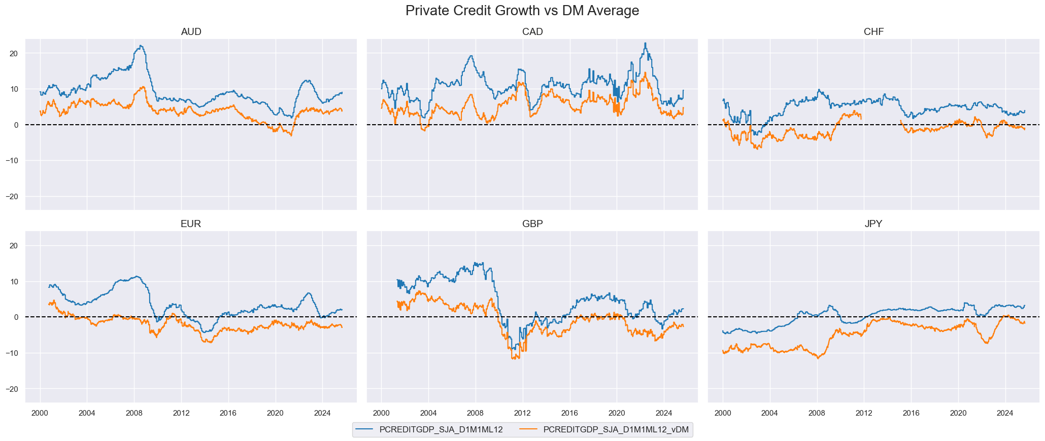
# Compare private credit growth to DM average
cidsx = cids_dm[:6]
xcat = "PCREDITGDP_SJA_D1M1ML12"

dfy = msp.make_relative_value(
    dfx,
    xcats=[xcat],
    cids=cidx,
    start="2000-01-01",
    blacklist=fxblack,
    rel_meth="subtract",
    complete_cross=False,
    postfix="_vDM",
)

dfx = msm.update_df(dfx, dfy)

msp.view_timelines(
    pd.concat([dfx[dfx["xcat"] == xcat], dfy]),
    xcats=[xcat, f"{xcat}_vDM"],
    cids=cidx,
    ncol=3,
    same_y=True,
    start="2000-01-01",
    title="Private Credit Growth vs DM Average",
    title_fontsize=20
)

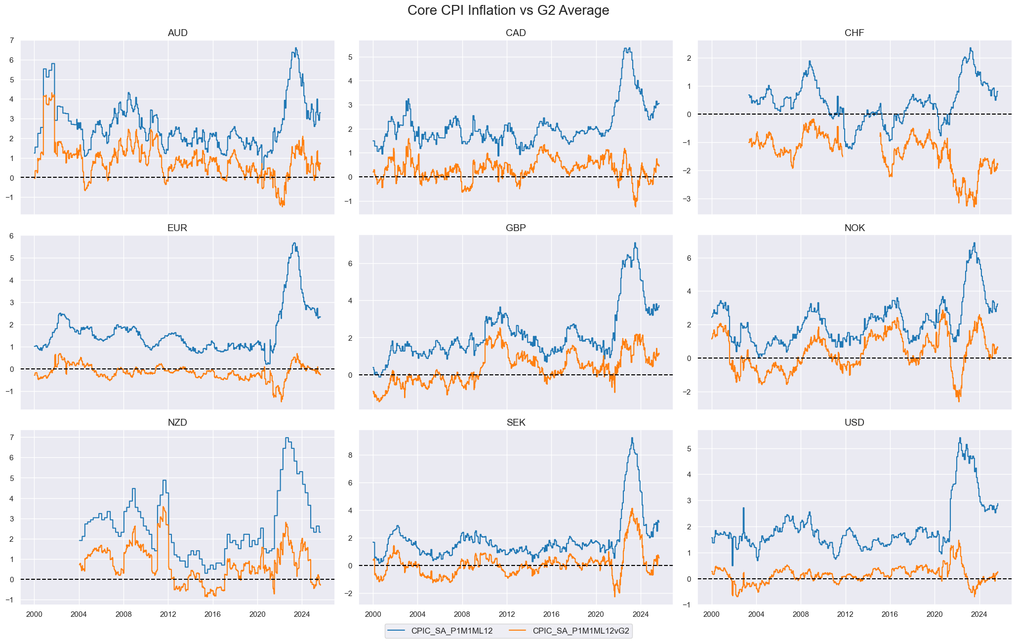
# Core CPI inflation relative to G2 (USD, EUR)
cidx = [cid for cid in cids_dm if cid != "JPY"]
xcat = "CPIC_SA_P1M1ML12"

dfy = msp.make_relative_value(
    dfx,
    xcats=[xcat],
    cids=cidx,
    start="2000-01-01",
    blacklist=fxblack,
    basket=["EUR", "USD"],
    rel_meth="subtract",
    postfix="vG2"
)

dfx = msm.update_df(dfx, dfy)

msp.view_timelines(
    dfx,
    xcats=[xcat, f"{xcat}vG2"],
    cids=cidx,
    ncol=3,
    same_y=False,
    start="2000-01-01",
    title="Core CPI Inflation vs G2 Average",
    title_fontsize=20
)

Normalize panels with make_zn_scores

The make_zn_scores() function standardizes values across categories using sequentially expanding estimates of means and deviations, ensuring the point-in-time property of the data is preserved. Unlike a traditional z-score, which is always centered around the mean, this function lets you specify a user-defined neutral level.

A zn-score is simply the normalized distance of a value from that chosen neutral point.

Important parameters include:

• sequential : If True , z-scores are computed step by step through time.

• neutral : The value considered as the benchmark. i.e. 'zero' , 'median' , 'mean' , or any number.

• pan_weight : Controls how much weight the overall panel has versus individual cross-sections when calculating z-score parameters (the neutral level and mean absolute deviation). The default is 1 , meaning parameters are based on the full panel. A value of 0 means parameters are calculated separately for each cross-section.

• thresh : A cutoff for zn-scores. The minimum threshold is 1 mean absolute deviation.

• min_obs : Minimum number of observations required to calculate z-scores.

• est_freq : Frequency at which z-scores are estimated. i.e 'D' (daily, default), 'W' (weekly), 'M' (monthly), 'Q' (quarterly).

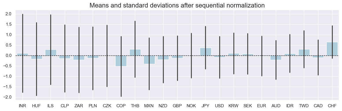
macros = ["XGDP_NEG", "XCPI_NEG", "XPCG_NEG", "RYLDIRS05Y_NSA"]

for xcat in macros:
    dfa = msp.make_zn_scores(
        dfx,
        xcat=xcat,
        cids=cids,
        neutral="zero",
        thresh=3,
        est_freq="M", # Month
        pan_weight=1,
        postfix="_ZN",
    )
    dfx = msm.update_df(dfx, dfa)

# Compare original and normalized GDP

cidx = [cid for cid in cids if cid not in ["TRY"]]

msp.view_ranges(
    dfx,
    xcats=["XCPI_NEG_ZN"],
    cids=cidx,
    kind="bar",
    sort_cids_by="std",
    start="2000-01-01",
    size=(12,4),
    title="Means and standard deviations after sequential normalization",
    title_fontsize=20)

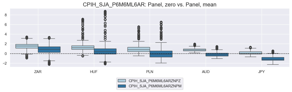
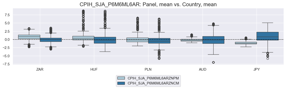
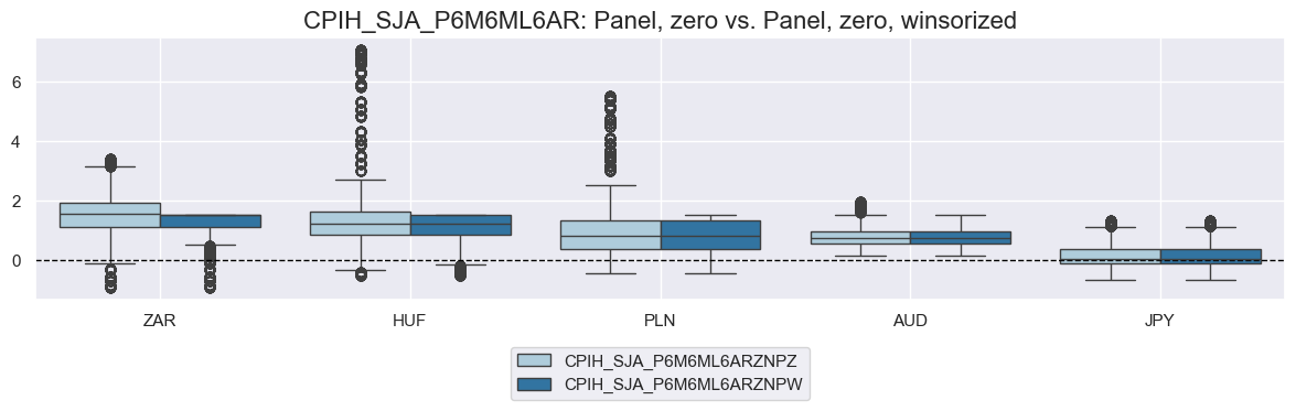
xcat = "CPIH_SJA_P6M6ML6AR"
cidx = ["ZAR", "HUF", "PLN", "AUD", "JPY"]

# Scoring variants
score_configs = {
    "ZNPZ": {"neutral": "zero",  "pan_weight": 1, "thresh": None,  "label": "Panel, zero"},
    "ZNPM": {"neutral": "mean",  "pan_weight": 1, "thresh": None,  "label": "Panel, mean"},
    "ZNCM": {"neutral": "mean",  "pan_weight": 0, "thresh": None,  "label": "Country, mean"},
    "ZNPW": {"neutral": "zero",  "pan_weight": 1, "thresh": 1.5,   "label": "Panel, zero, winsorized"},
}

dfy = pd.DataFrame(columns=dfx.columns)

for postfix, cfg in score_configs.items():
    dfa = msp.make_zn_scores(
        dfx,
        xcat=xcat,
        cids=cidx,
        sequential=True,
        neutral=cfg["neutral"],
        pan_weight=cfg["pan_weight"],
        thresh=cfg["thresh"],
        postfix=postfix,
        est_freq="m",
    )
    dfy = msm.update_df(dfy, dfa)

# Compare pairs of scoring methods
for pair in [("ZNPZ", "ZNPM"), ("ZNPM", "ZNCM"), ("ZNPZ", "ZNPW")]:
    msp.view_ranges(
        dfy,
        xcats=[f"{xcat}{pair[0]}", f"{xcat}{pair[1]}"],
        kind="box",
        sort_cids_by="mean",
        start="2000-01-01",
        size=(12, 4),
        title=f"{xcat}: {score_configs[pair[0]]['label']} vs. {score_configs[pair[1]]['label']}",
        title_fontsize=16
    )

Estimate and visualize hedged returns with return_beta

The return_beta() function estimates the beta (elasticity) of a return category with respect to a benchmark using simple OLS. It can return either the time series of betas or the hedged returns, i.e. the returns of a composite position that combines the asset and the benchmark to neutralize the asset’s benchmark exposure.

Important parameters include:

• reqfreq : how often the hedge ratios are recalculated. At the end of each chosen period, a new hedge ratio is estimated and then applied to all days in the next period. i.e. 'W' (weekly), 'M' (monthly, default), 'Q' (quarterly).

• min_obs : Minimum number of observations needed to calculate a beta. If the regression window is too short, no beta is produced.

• max_obs : Maximum number of observations to use. If there is more data available, the function cuts down on the sample.

• hedged_returns : If True , the function outputs hedged returns in addition to (or instead of) the betas.

• blacklist : Exclude specified cross-sections and time ranges from the regression

# Estimate hedge ratios and construct hedged FX returns
cidx = ["AUD", "CAD", "CHF", "EUR", "GBP", "JPY", "NOK", "NZD", "SEK"]

dfx = dfx[["cid", "xcat", "real_date", "value"]]  # drop unused columns

dfh = msp.return_beta(
    dfx,
    xcat="FXXR_NSA",
    cids=cidx,
    benchmark_return="USD_EQXR_NSA",
    oos=False,               # use in-sample beta estimation
    hedged_returns=True,
    start="2002-01-01",
    refreq="M"
)

dfx = msm.update_df(dfx, dfh)

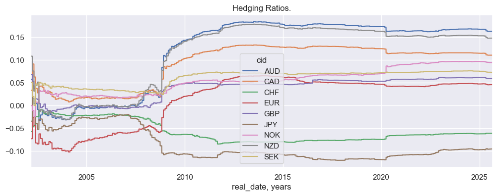
The beta_display() function provides a quick visualization of the estimated hedge ratios over time across cross-sections.

If the subplots parameter is set to True , the function creates one subplot per cross-section which is useful for comparing shapes or patterns individually without overlap.

If subplots=False (default), all betas are plotted together on the same axes, useful for spotting relative differences across cross-sections.

sns.set(rc={"figure.figsize": (12, 4)})
msp.beta_display(dfh)

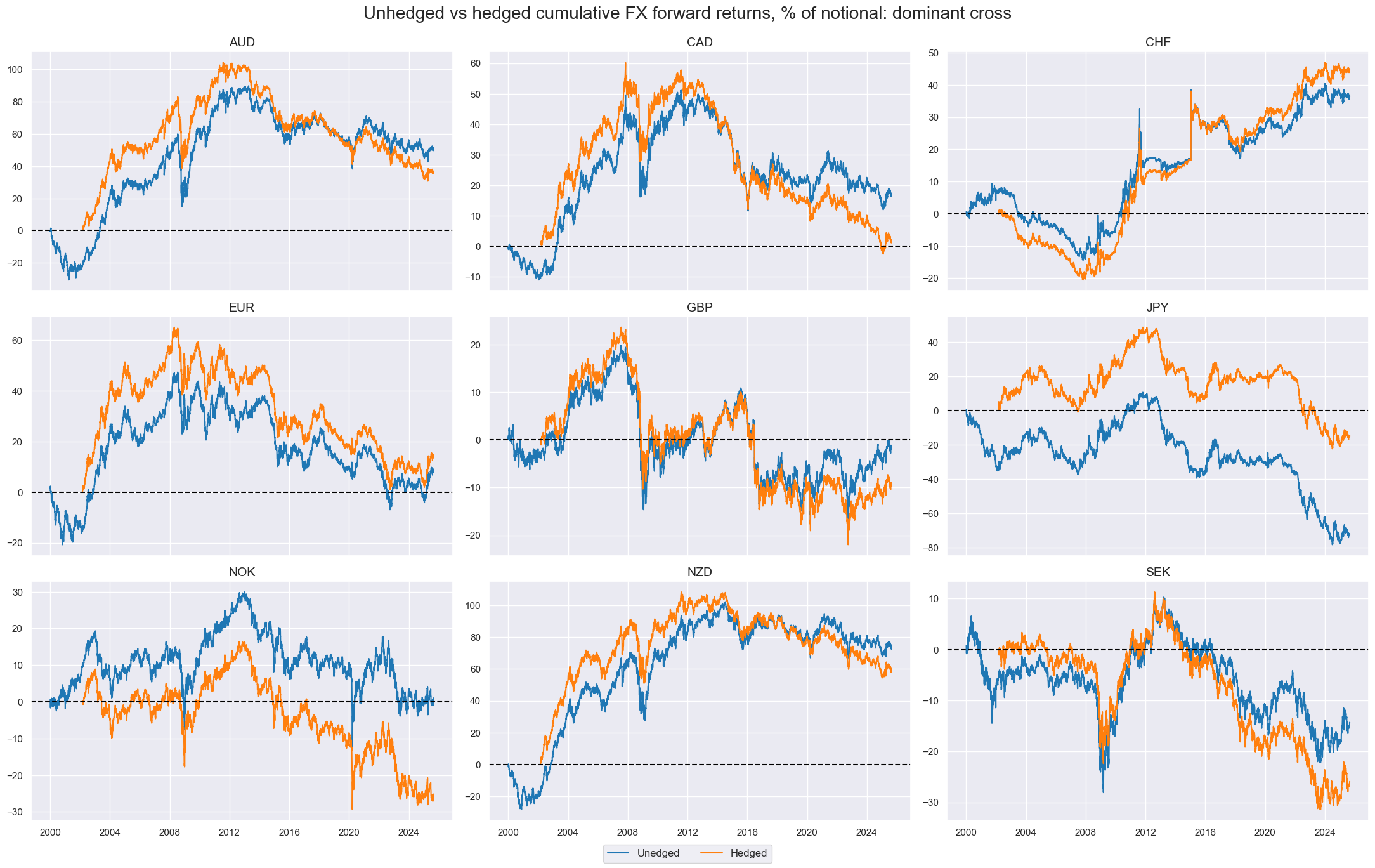
The view_timelines() function (introduced earlier in this notebook) can be used to visualize the cumulative differences between hedged and unhedged returns.

xcatx = ["FXXR_NSA", "FXXR_NSA_H"]

msp.view_timelines(
    dfx,
    xcats=xcatx,
    cids=cidx,
    ncol=3,
    cumsum=True,
    start="2000-01-01",
    same_y=False,
    all_xticks=False,
    title="Unhedged vs hedged cumulative FX forward returns, % of notional: dominant cross",
    xcat_labels=["Unedged", "Hedged"],
    height=3,
    title_fontsize=20
)

Generate returns (and carry) of a group of contracts with Basket

The Basket class calculates returns and carry for groups of financial contracts, applying different weighting methods.

The main input is a list of contracts, where each contract is defined as a combination of a cross-section and a category, representing a specific market and asset type.

Key parameters of the class:

• contracts : A list on cross-sections included in the Basket.

• ret : The return category to use when calculating basket return, this specifies which type of return data is aggregated into the basket performance.

• cry : The carry category to use alongside returns. Default is none.

• blacklist : A list of periods to exclude from the basket calculation.

In the example below, we create a Basket object for a set of FX forward returns.

# Define contracts for the basket (FX returns)
cids_fxcry = ["AUD", "INR", "NZD", "PLN", "TWD", "ZAR"]
contracts = [cid + "_FX" for cid in cids_fxcry]

# Create the basket object
basket_fxcry = msp.Basket(
    dfx,
    contracts=contracts,
    ret="XR_NSA",
    cry="CRR_NSA",
    start="2010-01-01",
    end="2023-01-01",
    blacklist=fxblack,
)

The make_basket() function calculates and stores performance metrics, returns and carry, using a chosen weighting method. The available weighting options provide flexibility to construct a composite measure tailored to your objectives.

The choices of the weight_meth parameter are:

• equal : Each contract gets the same weight, irregardless of volatility or size.

• fixed : You provide a fixed set of weights that remain constant.

• invsd : Weights are set to be inversely proportional to volatility.

  • lback_meth : How the variable used for weights is aggregated over time. i.e. 'ema' (Exponential moving average, default) or 'ma' (Simple moving average)

  • lblack_periods : Number of periods used for the look-back. Default is 21 .

• values : Weights are based on the absolute level of a chosen variable.

• inv_values : Weights are based on the inverse of the absolute level of a chosen variable.

basket_fxcry.make_basket(weight_meth="equal", basket_name="GLB_FXCRY")
basket_fxcry.make_basket(weight_meth="invsd", basket_name="GLB_FXCRYVW")
basket_fxcry.make_basket(
    weight_meth="fixed",
    weights=[1 / 3, 1 / 6, 1 / 12, 1 / 6, 1 / 3, 1 / 12],
    basket_name="GLB_FXCRYFW",
)

The return_basket() function returns the basket’s performance metrics in a standardized format.

dfb = basket_fxcry.return_basket()
print(dfb.tail())
utiks = list((dfb["cid"] + "_" + dfb["xcat"]).unique())
f"Unique basket tickers: {utiks}"

       real_date  cid             xcat     value
20341 2022-12-26  GLB  FXCRYFW_CRR_NSA -0.377433
20342 2022-12-27  GLB  FXCRYFW_CRR_NSA -0.397963
20343 2022-12-28  GLB  FXCRYFW_CRR_NSA -0.344370
20344 2022-12-29  GLB  FXCRYFW_CRR_NSA -0.253848
20345 2022-12-30  GLB  FXCRYFW_CRR_NSA  0.065548

"Unique basket tickers: ['GLB_FXCRY_XR_NSA', 'GLB_FXCRY_CRR_NSA', 'GLB_FXCRYVW_XR_NSA', 'GLB_FXCRYVW_CRR_NSA', 'GLB_FXCRYFW_XR_NSA', 'GLB_FXCRYFW_CRR_NSA']"

Use the return_weights() function to inspect the time series of weights used in the basket. These can be repurposed for feature weighting or diagnostics.

You pick the basket name or list of baskets for which you want performance data returned with the basket_names parameter.

dfw = basket_fxcry.return_weights()
weights_pivot = dfw.pivot_table(index="real_date", columns=["xcat", "cid"], values="value").replace(0, np.nan)
weights_pivot.tail(3).round(2)

xcat	FX_GLB_FXCRYFW_WGT						FX_GLB_FXCRYVW_WGT						FX_GLB_FXCRY_WGT
cid	AUD	INR	NZD	PLN	TWD	ZAR	AUD	INR	NZD	PLN	TWD	ZAR	AUD	INR	NZD	PLN	TWD	ZAR
real_date
2022-12-28	0.29	0.14	0.07	0.14	0.29	0.07	0.09	0.26	0.1	0.24	0.23	0.07	0.17	0.17	0.17	0.17	0.17	0.17
2022-12-29	0.29	0.14	0.07	0.14	0.29	0.07	0.09	0.27	0.1	0.23	0.23	0.07	0.17	0.17	0.17	0.17	0.17	0.17
2022-12-30	0.29	0.14	0.07	0.14	0.29	0.07	0.09	0.27	0.1	0.24	0.23	0.07	0.17	0.17	0.17	0.17	0.17	0.17

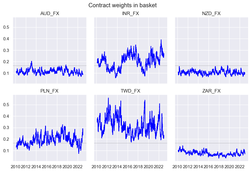
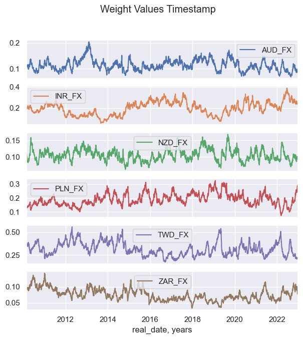
The weight_visualizer function visualizes weight allocations over time.

Important parameters are:

• subplots: If True , each contract is shown on a seperate plot and if False (default), all contracts are shown on a single plot.

• facet_grid: If True , splits the chart into multiple small coordinate grids when there are many contracts. False is the default.

• all_tickers: If True (default), all tickers are included in the visualization.

• single_tickers: Lets you zoom in on the weight of one specific contract. Only works if all_tickers=False .

basket_fxcry.weight_visualiser(basket_name="GLB_FXCRYVW", facet_grid=True)

basket_fxcry.weight_visualiser(basket_name="GLB_FXCRYVW", subplots=False, size=(10, 4))

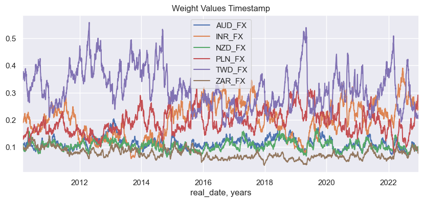
basket_fxcry.weight_visualiser(basket_name="GLB_FXCRYVW", subplots=True, )

Calculate linear combinations of panels with linear_composite

The linear_composite() function calculates linear combinations of different categories to produce a composite series. It can generate a composite even when some component data are missing, making it more flexible and practical. This is particularly useful when combining categories that capture a common underlying factor, since you can still work with the available information rather than discarding incomplete data.

Important parameters are:

• weights : How categories or cross-sections are combined in the composite. There are 3 main options:

  • None (default): All categories or cross-sections are given equal weights.

  • list of floats: You provide weights(e.g. [0.6, 0.4]), which are applied to all available categories or cross-sections. By default, these are normalized to sum to 1 per period, unless normalize_weights=False .

  • string: You can specify another category to use as a time-varying weight (e.g., GDP, market cap). The weight category is multiplied with the corresponding main category for each cross-section. By default, the weights are normalized to sum to 1 each period, unless normalize_weights=False .

• normalize_weights : If True (default), the weights are normalized to sum to 1.

• signs : An array indicating whether each component should enter with a positive or negative sign.

• complete_xcats / complete_cids : If True , all cross-sections/categories are required to be present at each time point.

The examples below show how to use linear_composite() in three ways:

• Combine two categories per cross-section (e.g. inflation metrics).

• Combine two cross-sections of one category (e.g. EUR vs USD inflation).

• Apply category-based weights (e.g. using GDP as weights).

If one of the inputs is missing at a given time, the function defaults to the available value.

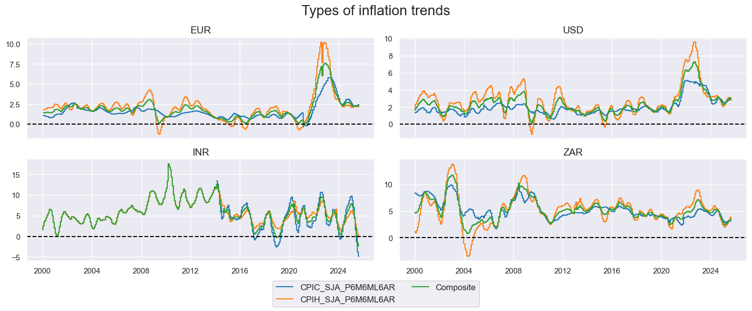
# Average core and headline inflation metrics by country
cidx = ["EUR", "USD", "INR", "ZAR"]
xcatx = ["CPIC_SJA_P6M6ML6AR", "CPIH_SJA_P6M6ML6AR"]

dflc = msp.linear_composite(
    df=dfx,
    xcats=xcatx,
    cids=cidx,
    weights=[1, 1],
    signs=[1, 1],
    complete_xcats=False,
    new_xcat="Composite"
)

dfx = msm.update_df(dfx, dflc)

msp.view_timelines(
    dfx,
    xcats=xcatx + ["Composite"],
    cids=cidx,
    ncol=2,
    start="1995-01-01",
    same_y=False,
    title="Types of inflation trends",
    aspect=2.5,
    height=2,
    title_fontsize=20
)

# Cross-sectional inflation gap: EUR minus USD
dflc = msp.linear_composite(
    df=dfx,
    xcats="CPIC_SJA_P6M6ML6AR",
    cids=["EUR", "USD"],
    weights=[1, 1],
    signs=[1, -1],
    complete_cids=False,
    start="2016-01-01",
    new_cid="EUR-USD"
)

dfx = msm.update_df(dfx, dflc)

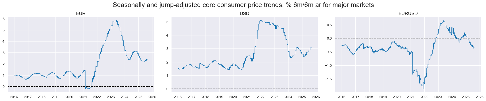
You can also use a category as a dynamic weight. Below, we use 5-year real GDP growth to weight the EUR vs USD inflation difference.

cidx = ["EUR", "USD"]
xcat="CPIC_SJA_P6M6ML6AR"
signs = [1, -1]

dflc = msp.linear_composite(
    df=dfx,
    start = "2016-01-01",
    xcats=xcat,
    cids=cidx,

    signs=signs,
    complete_cids=False,
    new_cid="EURUSD",
)

dfx = msm.update_df(dfx, dflc)

msp.view_timelines(
    df=dfx,
    xcats="CPIC_SJA_P6M6ML6AR",
    cids=cidx +["EURUSD"],
    ncol=4,
    start = "2016-01-01",
    same_y=False,
    title = "Seasonally and jump-adjusted core consumer price trends, % 6m/6m ar for major markets",
    title_fontsize=20
    
    )

macros = ["XGDP_NEG", "XCPI_NEG", "XPCG_NEG", "RYLDIRS05Y_NSA"]
xcatx = macros

dfa = msp.linear_composite(
    dfx,
    xcats=[xc + "_ZN" for xc in xcatx],
    cids=cids,
    new_xcat="MACRO_AVGZ",
)

dfx = msm.update_df(dfx, dfa)

Relating

Investigate relations between panels with CategoryRelations

The CategoryRelations class is a tool for quickly visualizing and analyzing the relationship between two category panels (time-series). You can specify key arguments such as the analysis period and the type of aggregation, which determine how the relationship is calculated and displayed.

Key arguments:

• freq : Frequency at which the series are to be sampled. i.e. 'D' , 'W' , 'M' (default), 'Q' , 'A' .

• years : Specifies the number of years over which data should be aggregated. This overrides the freq parameter and cannot be combined with lags. The default is None , and the function uses whatever freq you specify.
  
  

• fwin : Length of the forward-looking moving average window for the second category. Default is 1 .

• blacklist : Cross-sections and time periods to exclude.

• slip : How many periods to shift (‘slip’) the explanatory variable (first category). This simulates delays such as data being published late or taking time to act upon. Default is 0 .
  
  

• xcat_aggs : The two aggregation methods you want to use. Default is 'mean' for both. Others include 'median' , 'sum' , 'min' , 'max' , etc.

• xcat_trims : The two maximum absolute values allowed for each of the two categories. Any observations exceeding these thresholds are removed entirely from the analysis (trimmed). Default is None for both. Trimming happens only after all other transformations have been completed.

• xcat1_chg : Specification whether to transform the first category into changes rather than levels. Default is None . The available options are:

  • 'diff' : Calculates the first difference

  • 'pch' : Calculates the percentage change

• n_periods : Number of periods used when calculating changes in the first category (set by xcat1_chg ). Default is 1 .

cr = msp.CategoryRelations(
    dfx,
    xcats=["CPIC_SJA_P6M6ML6AR", "DU05YXR_VT10"],
    cids=cids_dm,
    xcat1_chg="diff",
    n_periods=1,
    freq="Q",
    lag=1,
    fwin=1,  # default forward window is one
    xcat_aggs=["last", "sum",],  # the first method refers to the first item in xcats list, the second - to the second
    start="2000-01-01",
    xcat_trims=[10, 10],
)

for attribute, value in cr.__dict__.items():
    print(attribute, " = ", value)

xcats  =  ['CPIC_SJA_P6M6ML6AR', 'DU05YXR_VT10']
cids  =  ['AUD', 'CAD', 'CHF', 'EUR', 'GBP', 'JPY', 'NOK', 'NZD', 'SEK', 'USD']
val  =  value
freq  =  Q
lag  =  1
years  =  None
aggs  =  ['last', 'sum']
xcat1_chg  =  diff
n_periods  =  1
xcat_trims  =  [10, 10]
slip  =  0
df  =                  CPIC_SJA_P6M6ML6AR  DU05YXR_VT10
real_date  cid                                  
2001-12-31 AUD            1.135315     -3.172330
2002-03-29 AUD            0.446704     -3.966165
2002-06-28 AUD           -0.575002      3.346755
2002-09-30 AUD            0.233650      7.388278
2002-12-31 AUD            0.203154      2.739271
...                            ...           ...
2024-09-30 CHF            0.383461      8.498372
2024-12-31 CHF           -0.185516      7.098018
2025-03-31 CHF           -0.443607     -4.128092
2025-06-30 CHF           -0.130310      3.260313
2025-09-30 CHF            0.123553     -0.046946

[812 rows x 2 columns]

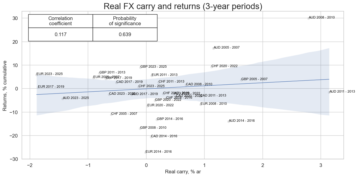
Plot regression scatter with reg_scatter

The reg_scatter() function visualizes the relationship between two categories by displaying a scatter-plot, making it easy to see both the strength of the association and potential outliers. The analysis can also be split by cid (cross-section) or year , helping to reveal how the relationship changes across markets or over time.

Important parameters:

• fit_reg : If True , adds a regression line.

• prob_est : Type of estimator to use for calculating the probability of a significant relationship between the feature category and the target category. Options are:

  • pool (default): Pools all cross-sections and periods together into one regression.

  • map : (Macrosynergy panel test) where significance is assessed using panel regressions with period-specific random effects. This avoids the problem of ‘pseudo-replication’ that arises when simply stacking data, which can exaggerate significance because cross-sections often share common global factors. The method adjusts both targets and features for these global influences, giving more weight to deviations from the period mean. In practice, if global effects dominate, the test focuses on whether a feature explains cross-sectional differences at each point in time. This approach automatically accounts for similarity across markets, making the significance test more reliable and broadly applicable.

  • kendall : Kendall rank correlation coefficient.

The years parameter, when combined with labels=true , can be used to visualize medium-term concurrent relations.

cids_sel = cids_dm[:5]
cr = msp.CategoryRelations(
    df,
    xcats=["FXCRR_NSA", "FXXR_NSA"],
    cids=cids_sel,
    freq="M",
    years=3,
    lag=0,
    xcat_aggs=["mean", "sum"],
    start="2005-01-01",
    blacklist=fxblack,
)
cr.reg_scatter(
    title="Real FX carry and returns (3-year periods)",
    title_fontsize=20,
    labels=True,
    prob_est="map",
    xlab="Real carry, % ar",
    ylab="Returns, % cumulative",
    coef_box="upper left",
    size=(12, 6),
)

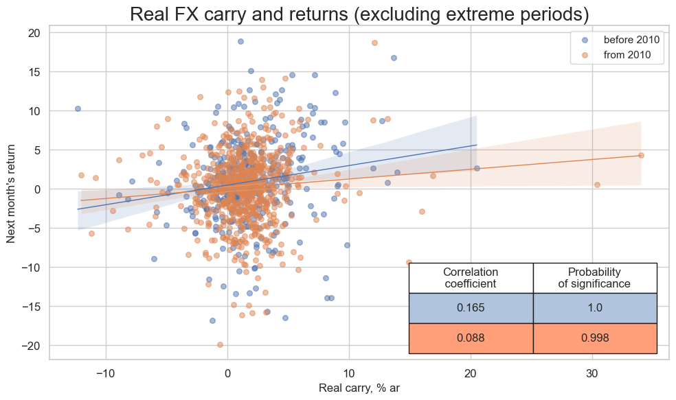
The separator argument is used to check whether a relationship remains stable across different time periods or markets.

In practice, it splits the scatter plots either by cross-section ( cids ) or by time, such as calendar year ( year ).

cidx = cids_em

cr = msp.CategoryRelations(
    dfx,
    xcats=["FXCRR_NSA", "FXXR_NSA"],
    cids=list(set(cids_em) - set(["ILS", "CLP"])),
    freq="Q",
    years=None,
    lag=1,
    xcat_aggs=["last", "sum"],
    start="2000-01-01",
    blacklist=fxblack,
    xcat_trims=[40, 20],
)
cr.reg_scatter(
    title="Real FX carry and returns (excluding extreme periods)",
    title_fontsize=20,
    reg_order=1,
    labels=False,
    xlab="Real carry, % ar",
    ylab="Next month's return",
    coef_box="lower right",
    prob_est="map",
    separator=2010,
    size=(10, 6),
)

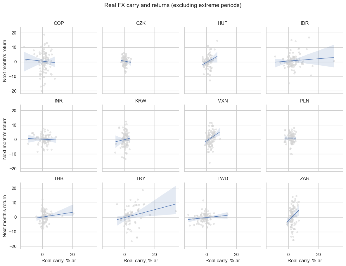
cr.reg_scatter(
    title="Real FX carry and returns (excluding extreme periods)",
    reg_order=1,
    labels=False,
    xlab="Real carry, % ar",
    ylab="Next month's return",
    separator="cids",
    tick_fontsize=20,
    title_adj=1.01,
)

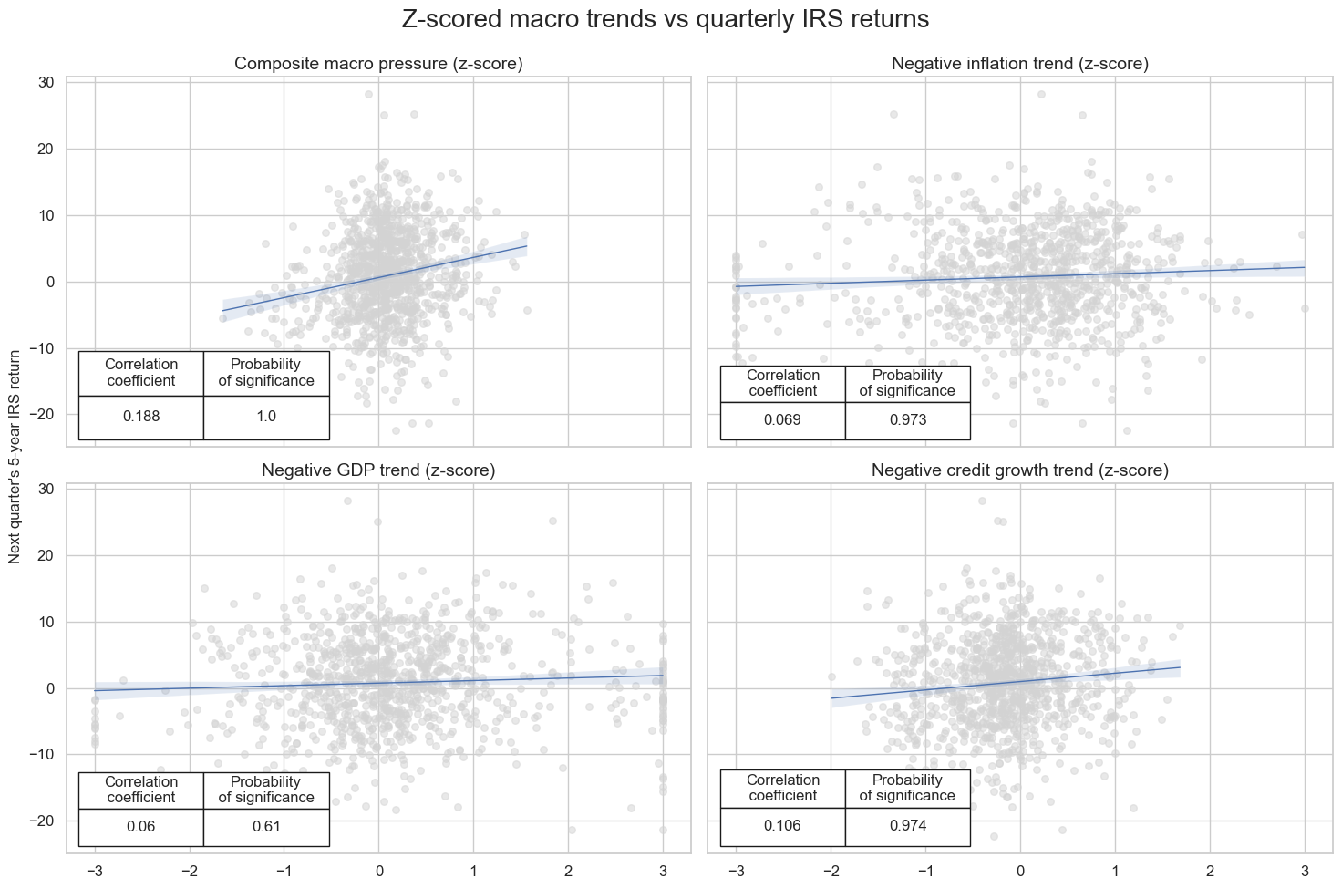
The multiple_reg_scatter() function is for comparison of several pairs of two categories relationships side by side, including the strength of the linear association and any potential outliers.

Important parameters:

• cat_rels : List of category relationships to plot.

• share_axes : If True , the plots share their axes. Default is False .

• coef_box : If True , displays a summary box for each scatter-plot showing: the estimated regression coefficient, it’s standard error, and significance level. Default is False .

crx = msp.CategoryRelations(
    dfx,
    xcats=["MACRO_AVGZ", "DU05YXR_VT10"],
    cids=cids_dm,
    n_periods=1,
    freq="Q",
    lag=1,
    xcat_aggs=["last", "sum"],
    start="2000-01-01",
)

crxx = msp.CategoryRelations(
    dfx,
    xcats=["XCPI_NEG_ZN", "DU05YXR_VT10"],
    cids=cids_dm,
    n_periods=1,
    freq="Q",
    lag=1,
    xcat_aggs=["last", "sum"],
    start="2000-01-01",
)

crxxx = msp.CategoryRelations(
    dfx,
    xcats=["XGDP_NEG_ZN", "DU05YXR_VT10"],
    cids=cids_dm,
    n_periods=1,
    freq="Q",
    lag=1,
    xcat_aggs=["last", "sum"],
    start="2000-01-01",
)

crxxxx = msp.CategoryRelations(
    dfx,
    xcats=["XPCG_NEG_ZN", "DU05YXR_VT10"],
    cids=cids_dm,
    n_periods=1,
    freq="Q",
    lag=1,
    xcat_aggs=["last", "sum"],
    start="2000-01-01",
)

msv.multiple_reg_scatter(
    [crx, crxx, crxxx, crxxxx],
    title="Z-scored macro trends vs quarterly IRS returns",
    ylab="Next quarter's 5-year IRS return",
    ncol=2,
    nrow=2,
    figsize=(15, 10),
    prob_est="map",
    coef_box="lower left",
    subplot_titles=[
        "Composite macro pressure (z-score)",
        "Negative inflation trend (z-score)",
        "Negative GDP trend (z-score)",
        "Negative credit growth trend (z-score)",
    ],
)

Call the .ols_table() function to run a basic pooled OLS regression and return a statsmodels summary.

cr = msp.CategoryRelations(
    dfx,
    xcats=["CPIC_SJA_P6M6ML6AR", "DU05YXR_VT10"],
    cids=cids_dm,
    xcat1_chg="diff",
    n_periods=1,
    freq="M",
    lag=1,
    xcat_aggs=["last", "sum"],
    start="2000-01-01",
)
cr.ols_table()

                            OLS Regression Results                            
==============================================================================
Dep. Variable:           DU05YXR_VT10   R-squared:                       0.000
Model:                            OLS   Adj. R-squared:                  0.000
Method:                 Least Squares   F-statistic:                     1.262
Date:                Mon, 01 Sep 2025   Prob (F-statistic):              0.261
Time:                        12:35:00   Log-Likelihood:                -7890.4
No. Observations:                2896   AIC:                         1.578e+04
Df Residuals:                    2894   BIC:                         1.580e+04
Df Model:                           1                                         
Covariance Type:            nonrobust                                         
======================================================================================
                         coef    std err          t      P>|t|      [0.025      0.975]
--------------------------------------------------------------------------------------
const                  0.2439      0.069      3.554      0.000       0.109       0.378
CPIC_SJA_P6M6ML6AR    -0.3380      0.301     -1.123      0.261      -0.928       0.252
==============================================================================
Omnibus:                      187.185   Durbin-Watson:                   1.806
Prob(Omnibus):                  0.000   Jarque-Bera (JB):              660.911
Skew:                          -0.244   Prob(JB):                    3.05e-144
Kurtosis:                       5.289   Cond. No.                         4.39
==============================================================================

Notes:
[1] Standard Errors assume that the covariance matrix of the errors is correctly specified.

Visualize relations across sections or categories with correl_matrix

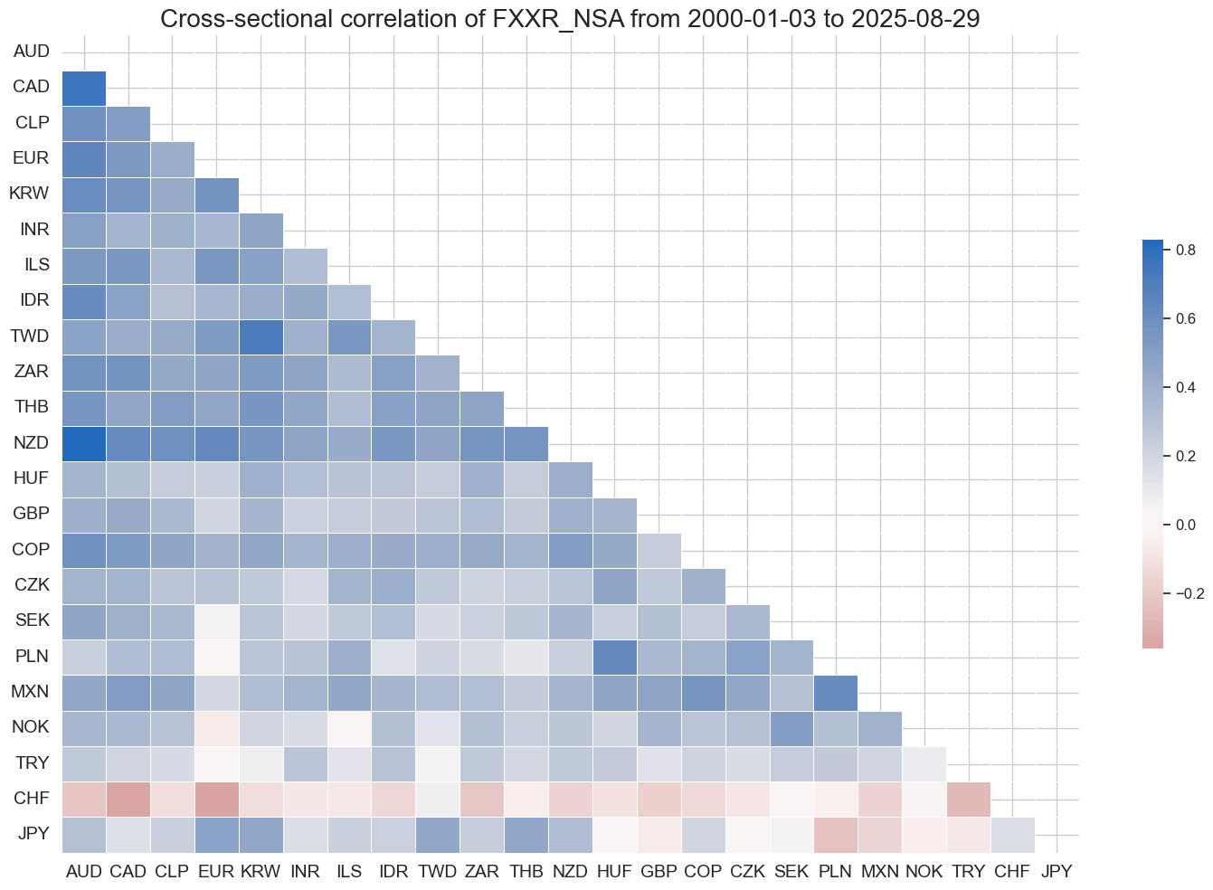
The correl_matrix() function visualizes Pearson correlations in two ways:

• Within a single category across multiple cross-sections.

• Across different categories. This makes it easy to spot common patterns or overlaps either between markets or between signals.

Important parameters:

• freq : Frequency at which the standard JMPaQS frequency of business daily data is downsampled to. i.e 'W' , 'M' (default), or 'Q' .

• cluster : If True , the series in the correlation matrix are reordered using hierarchical clustering, so assets or categories with similar correlation patterns are grouped together. Default is False .

cids = cids_dm + cids_em
msp.correl_matrix(
    dfx, xcats="FXXR_NSA", 
    freq="Q", 
    cids=cids, 
    size=(15, 10), 
    cluster=True,
    title_fontsize=20
)

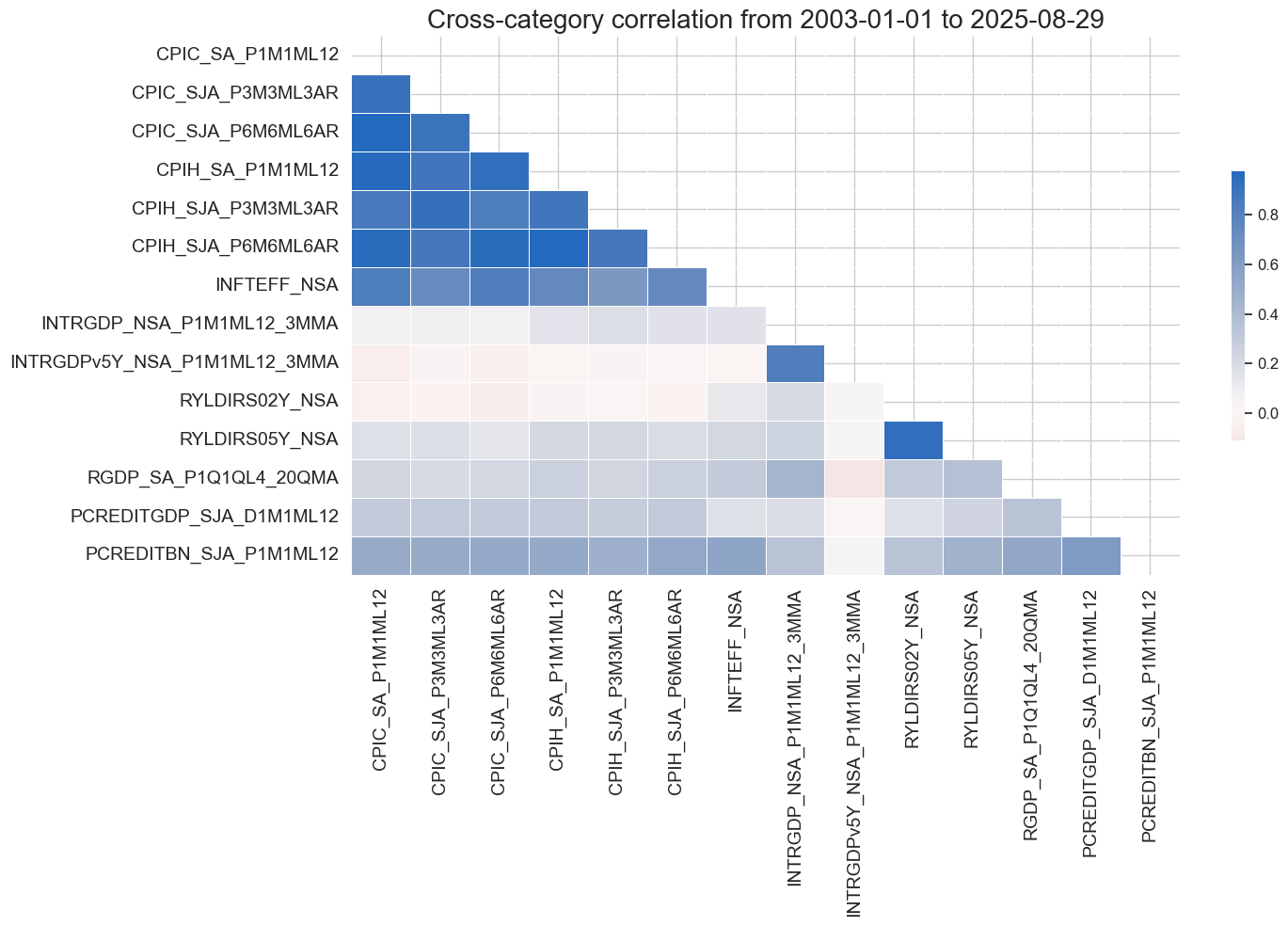
Passing a list of categories to the xcats argument to display correlations across categories:

xcatx = ecos
msp.correl_matrix(
    dfx,
    xcats=xcatx,
    cids=cids,
    freq="M",
    start="2003-01-01",
    size=(15, 10),
    cluster=True,
    title_fontsize=20
)

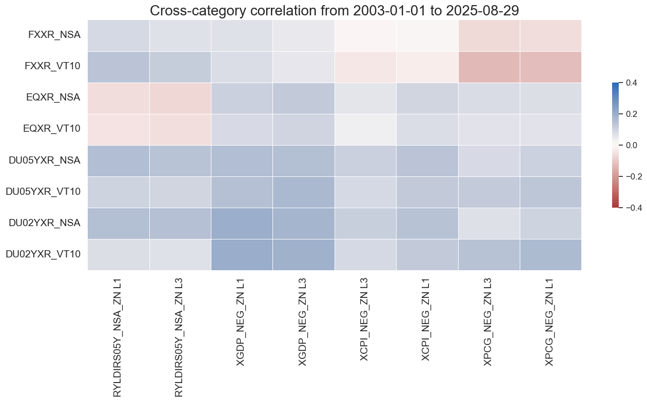
In the example below we analyze correlations between inflation trends and subsequent asset returns, allowing for multiple explanatory lags. Lags are passed as a dictionary so we can test several horizons in one go. Here, we use monthly lags of 1, 3, and 6 months:

macroz = [m + "_ZN" for m in macros]
feats = macroz

rets=["DU02YXR_VT10",
    "DU02YXR_NSA",
    "DU05YXR_VT10",
    "DU05YXR_NSA",
     "EQXR_NSA",
    "EQXR_VT10",
    "FXXR_NSA",
    "FXXR_VT10"]

lag_dict = {"XGDP_NEG_ZN": [1, 3], 
    "XCPI_NEG_ZN": [1, 3], # excess inflation
    "XPCG_NEG_ZN": [1, 3],  # excess real interest rate
    "RYLDIRS05Y_NSA_ZN": [1, 3]}


msp.correl_matrix(
    dfx,
    xcats=feats,
    xcats_secondary=rets, 
    cids="EUR",
    freq="M",
    start="2003-01-01",
    lags=lag_dict,
    max_color=0.4,
    cluster=True, 
    title_fontsize=20
)

Signaling

SignalReturnRelations

The SignalReturnRelations class is built to analyze, visualize, and compare how panels of trading signals relate to panels of subsequent returns. Unlike CategoryRelations, it focuses on association measures such as positive/negative return splits and both parametric and non-parametric correlations.

The class converts data to a chosen trading or rebalancing frequency and accounts for whether a signal is expected to predict returns with a positive or negative sign, which is crucial for interpreting results. Importantly, no regressions are run: features must have a meaningful zero point, since the sign of the signal directly drives the accuracy statistics.

Important parameters:

• rets : Target return category/categories.

• sigs : Signal categories for which detailed relational statistics can be calculated.

• sig_neg : List of True / False in relation to the list of signals. Default is False .

• agg_sigs : Aggregation method for down-sampling to a lower frequency. Default is 'last' . Options include 'mean' , 'median' , and 'sum' . If a single method is provided for multiple signal categories, it is applied to all of them.

• freqs : All frequencies at which the series can be sampled. i.e. 'D' , 'W' , 'M' (default), 'Q' , and 'A' . Return series are always summed over the selected period, while signal series are aggregated using the method(s) specified in agg_sigs .

dfx

	cid	xcat	real_date	value
0	AUD	CPIC_SA_P1M1ML12	2000-01-03	1.244168
1	AUD	CPIC_SA_P1M1ML12	2000-01-04	1.244168
2	AUD	CPIC_SA_P1M1ML12	2000-01-05	1.244168
3	AUD	CPIC_SA_P1M1ML12	2000-01-06	1.244168
4	AUD	CPIC_SA_P1M1ML12	2000-01-07	1.244168
...	...	...	...	...
5958343	ZAR	XXRYLD	2025-08-25	3.186982
5958344	ZAR	XXRYLD	2025-08-26	3.201803
5958345	ZAR	XXRYLD	2025-08-27	3.221633
5958346	ZAR	XXRYLD	2025-08-28	3.191177
5958347	ZAR	XXRYLD	2025-08-29	3.199969

5958348 rows × 4 columns

# Instantiate signal-return relations class for the list of signals, multiple returns and frequencies

srr = mss.SignalReturnRelations(
    dfx,
    sigs=["MACRO_AVGZ", "XGDP_NEG_ZN", "XCPI_NEG_ZN", "XPCG_NEG_ZN", "RYLDIRS05Y_NSA_ZN"],
    cosp=True,
    rets=["DU05YXR_VT10", "EQXR_VT10", "FXXR_VT10"],
    freqs=["M"],
    blacklist=fxblack,
    slip=1
)

Signal-return analysis

The view_grades() function displays a heatmap of data quality grades across time and cross-sections.

xcat_gr = "CPIH_SA_P1M1ML12"
df_gr = df[(df["xcat"] == xcat_gr) & (df["cid"].isin(cids_dm))].copy()

msv.view_grades(
    df_gr,
    xcats=[xcat_gr],
    cids=cids_dm,
    start="2000-01-01",
    end="2020-01-01",
    grade="grading",  # already present in df (float64)
    title="Grading quality of headline CPI inflation",
    title_fontsize=20,
    figsize=(13, 1)
)

Summary tables

The summary_table() function gives a quick snapshot of how well the main signal aligns with future returns. It shows classification accuracy, return bias, precision, and both linear and rank correlations; across the full panel, by year, and by cross-section.

The columns of the summary table:

• accuracy : % of correct sign predictions (positive vs negative returns). Ignores imbalance between up/down returns.

• bal_accuracy : balanced accuracy = average of true positive rate (sensitivity) and true negative rate (specificity). Adjusts for class imbalance. Range 0-1.

• pos_sigr : proportion of times the signal predicts a positive return (measures long bias of the signal).

• pos_retr : proportion of positive returns in the dataset (measures bias of the returns themselves).

• pos_prec : positive precision = % of positive return predictions that were correct. Range 0-1.

• neg_prec : negative precision = % of negative return predictions that were correct. Range 0-1.

• pearson : Pearson correlation coefficient between signal and subsequent returns (linear association, -1 to +1).

• pearson_pval : p-value for testing whether Pearson correlation ≠ 0 (probability result occurred by chance).

• kendall : Kendall rank correlation (non-parametric measure of monotonic association, -1 to +1).

• kendall_pval : p-value for Kendall correlation significance.

The rows of the summary table:

• Panel : statistic across the entire dataset (all cross-sections and sample period, excluding blacklisted data).

• Mean years : average value of the statistic across years.

• Mean cids : average value across cross-sections (e.g., countries, assets).

• Positive ratio : proportion of years (or cross-sections) where the statistic is above its neutral benchmark:

  • Neutral = 0.5 for classification stats (accuracy, balanced accuracy, precision).

  • Neutral = 0 for correlation measures (Pearson, Kendall).

srr.summary_table().round(2)

	accuracy	bal_accuracy	pos_sigr	pos_retr	pos_prec	neg_prec	pearson	pearson_pval	kendall	kendall_pval	auc
M: MACRO_AVGZ/last => DU05YXR_VT10	0.55	0.54	0.58	0.55	0.58	0.50	0.11	0.00	0.06	0.00	0.54
Mean years	0.54	0.52	0.59	0.56	0.57	0.46	0.06	0.35	0.03	0.32	0.52
Positive ratio	0.81	0.73	0.65	0.73	0.77	0.46	0.85	0.58	0.77	0.65	0.73
Mean cids	0.55	0.54	0.58	0.54	0.58	0.51	0.10	0.24	0.06	0.28	0.54
Positive ratio	0.83	0.83	0.71	0.92	0.92	0.54	0.96	0.79	0.92	0.71	0.83

Use the single_relation_table() function for a compact one-line summary showing frequency, signal (with _NEG if inverse), and return name.

srr.single_relation_table().round(2)

	accuracy	bal_accuracy	pos_sigr	pos_retr	pos_prec	neg_prec	pearson	pearson_pval	kendall	kendall_pval	auc
M: MACRO_AVGZ/last => DU05YXR_VT10	0.55	0.54	0.58	0.55	0.58	0.5	0.11	0.0	0.06	0.0	0.54

The cross_section_table() function summarizes accuracy and correlation stats by country and panel average.

It also shows the share of countries with positive signal-return relationships.

srr.cross_section_table().round(2)

	accuracy	bal_accuracy	pos_sigr	pos_retr	pos_prec	neg_prec	pearson	pearson_pval	kendall	kendall_pval	auc
M: MACRO_AVGZ/last => DU05YXR_VT10	0.55	0.54	0.58	0.55	0.58	0.50	0.11	0.00	0.06	0.00	0.54
Mean	0.55	0.54	0.58	0.54	0.58	0.51	0.10	0.24	0.06	0.28	0.54
PosRatio	0.83	0.83	0.71	0.92	0.92	0.54	0.96	0.79	0.92	0.71	0.83
AUD	0.56	0.54	0.59	0.57	0.61	0.48	0.13	0.03	0.05	0.17	0.54
CAD	0.52	0.52	0.57	0.51	0.52	0.51	0.05	0.38	0.02	0.58	0.52
CHF	0.58	0.56	0.69	0.56	0.60	0.52	0.14	0.02	0.08	0.05	0.55
CLP	0.48	0.48	0.49	0.51	0.50	0.47	0.06	0.36	0.02	0.73	0.48
COP	0.54	0.54	0.47	0.53	0.57	0.51	-0.05	0.55	0.02	0.65	0.54
CZK	0.51	0.51	0.42	0.54	0.56	0.47	0.08	0.23	0.02	0.61	0.51
EUR	0.57	0.56	0.58	0.57	0.62	0.50	0.20	0.00	0.12	0.00	0.56
GBP	0.55	0.54	0.62	0.56	0.59	0.50	0.21	0.00	0.09	0.02	0.54
HUF	0.59	0.59	0.65	0.51	0.58	0.60	0.14	0.02	0.09	0.02	0.58
IDR	0.66	0.63	0.67	0.63	0.72	0.55	0.22	0.00	0.18	0.00	0.63
ILS	0.53	0.50	0.65	0.59	0.59	0.41	0.02	0.82	-0.01	0.88	0.50
INR	0.47	0.47	0.55	0.49	0.46	0.48	0.04	0.57	-0.01	0.84	0.47
JPY	0.49	0.47	0.59	0.57	0.54	0.40	0.06	0.29	0.02	0.59	0.47
KRW	0.60	0.61	0.67	0.52	0.59	0.62	0.15	0.02	0.08	0.06	0.60
MXN	0.53	0.53	0.54	0.55	0.58	0.48	0.03	0.61	0.06	0.17	0.53
NOK	0.50	0.50	0.50	0.53	0.53	0.47	0.12	0.04	0.06	0.11	0.50
NZD	0.57	0.56	0.73	0.55	0.58	0.54	0.17	0.00	0.09	0.01	0.55
PLN	0.56	0.55	0.59	0.55	0.59	0.50	0.21	0.00	0.10	0.01	0.55
SEK	0.59	0.58	0.57	0.58	0.65	0.51	0.18	0.00	0.12	0.00	0.58
THB	0.60	0.59	0.69	0.56	0.62	0.56	0.01	0.89	0.05	0.31	0.58
TRY	0.57	0.56	0.32	0.46	0.55	0.57	0.10	0.27	0.05	0.37	0.55
TWD	0.50	0.51	0.47	0.52	0.53	0.48	0.07	0.26	0.03	0.44	0.51
USD	0.57	0.57	0.49	0.53	0.60	0.54	0.08	0.17	0.06	0.13	0.57
ZAR	0.54	0.52	0.72	0.57	0.58	0.46	0.09	0.13	0.07	0.06	0.51

The yearly_table() function breaks down signal performance by year, assessing consistency over time.

srr.yearly_table().round(2)

	accuracy	bal_accuracy	pos_sigr	pos_retr	pos_prec	neg_prec	pearson	pearson_pval	kendall	kendall_pval	auc
M: MACRO_AVGZ/last => DU05YXR_VT10	0.55	0.54	0.58	0.55	0.58	0.50	0.11	0.00	0.06	0.00	0.54
Mean	0.54	0.52	0.59	0.56	0.57	0.46	0.06	0.35	0.03	0.32	0.52
PosRatio	0.81	0.73	0.65	0.73	0.77	0.46	0.85	0.58	0.77	0.65	0.73
2000	0.51	0.53	0.46	0.78	0.81	0.26	0.10	0.40	0.06	0.45	0.55
2001	0.46	0.37	0.74	0.61	0.55	0.20	0.04	0.61	-0.06	0.32	0.40
2002	0.60	0.49	0.81	0.67	0.66	0.31	0.04	0.56	0.06	0.24	0.49
2003	0.49	0.43	0.81	0.55	0.52	0.34	-0.03	0.72	-0.02	0.65	0.46
2004	0.56	0.51	0.68	0.63	0.64	0.39	0.05	0.51	0.05	0.35	0.51
2005	0.52	0.52	0.52	0.51	0.53	0.51	0.04	0.61	-0.00	0.97	0.52
2006	0.49	0.48	0.34	0.48	0.45	0.51	-0.04	0.56	-0.06	0.16	0.48
2007	0.60	0.58	0.36	0.43	0.54	0.63	0.08	0.24	0.06	0.19	0.58
2008	0.51	0.58	0.29	0.63	0.74	0.41	0.21	0.00	0.14	0.00	0.57
2009	0.51	0.54	0.88	0.48	0.49	0.59	0.05	0.39	0.08	0.07	0.52
2010	0.63	0.58	0.75	0.64	0.68	0.49	0.12	0.04	0.10	0.01	0.57
2011	0.53	0.51	0.59	0.63	0.64	0.38	-0.10	0.09	-0.02	0.64	0.51
2012	0.54	0.53	0.57	0.58	0.60	0.46	0.05	0.41	0.04	0.37	0.53
2013	0.52	0.52	0.69	0.50	0.51	0.53	0.08	0.21	0.05	0.23	0.52
2014	0.60	0.55	0.62	0.72	0.76	0.35	0.12	0.06	0.10	0.02	0.56
2015	0.56	0.57	0.77	0.53	0.56	0.58	0.10	0.11	0.06	0.11	0.55
2016	0.50	0.50	0.64	0.49	0.49	0.51	0.03	0.62	0.03	0.51	0.50
2017	0.55	0.56	0.41	0.51	0.58	0.53	0.15	0.01	0.06	0.11	0.55
2018	0.46	0.46	0.42	0.51	0.47	0.45	0.02	0.72	0.00	0.95	0.46
2019	0.54	0.51	0.64	0.60	0.61	0.42	0.02	0.69	0.03	0.45	0.51
2020	0.59	0.45	0.85	0.67	0.66	0.24	-0.05	0.40	-0.10	0.01	0.47
2021	0.53	0.52	0.47	0.37	0.40	0.65	0.07	0.23	0.00	0.94	0.52
2022	0.69	0.49	0.08	0.27	0.26	0.73	0.07	0.24	0.06	0.16	0.50
2023	0.54	0.56	0.32	0.55	0.64	0.49	0.09	0.14	0.07	0.07	0.56
2024	0.57	0.58	0.83	0.54	0.57	0.60	0.05	0.37	0.05	0.22	0.55
2025	0.57	0.55	0.79	0.56	0.58	0.51	0.15	0.03	0.08	0.08	0.53

Use the multiple_relations_table() function to compare multiple signals (and/or frequencies) against a return series in one table.
Each row shows a signal-return pair with its frequency and standard metrics.

srr.multiple_relations_table().round(2)

				accuracy	bal_accuracy	pos_sigr	pos_retr	pos_prec	neg_prec	pearson	pearson_pval	kendall	kendall_pval	auc
Return	Signal	Frequency	Aggregation
DU05YXR_VT10	MACRO_AVGZ	M	last	0.55	0.54	0.58	0.54	0.58	0.51	0.10	0.00	0.06	0.00	0.54
	RYLDIRS05Y_NSA_ZN	M	last	0.55	0.54	0.71	0.54	0.56	0.51	0.08	0.00	0.05	0.00	0.53
	XCPI_NEG_ZN	M	last	0.53	0.53	0.54	0.54	0.56	0.49	0.04	0.00	0.03	0.00	0.53
	XGDP_NEG_ZN	M	last	0.52	0.51	0.55	0.54	0.55	0.48	0.04	0.00	0.03	0.00	0.51
	XPCG_NEG_ZN	M	last	0.52	0.53	0.36	0.54	0.58	0.48	0.06	0.00	0.05	0.00	0.53
EQXR_VT10	MACRO_AVGZ	M	last	0.53	0.51	0.58	0.59	0.60	0.42	0.05	0.00	0.03	0.01	0.51
	RYLDIRS05Y_NSA_ZN	M	last	0.51	0.47	0.67	0.59	0.57	0.37	-0.06	0.00	-0.04	0.00	0.47
	XCPI_NEG_ZN	M	last	0.54	0.53	0.55	0.59	0.62	0.44	0.08	0.00	0.05	0.00	0.53
	XGDP_NEG_ZN	M	last	0.51	0.50	0.55	0.59	0.60	0.41	0.03	0.07	0.01	0.60	0.50
	XPCG_NEG_ZN	M	last	0.48	0.50	0.38	0.59	0.60	0.41	0.02	0.14	0.02	0.09	0.50
FXXR_VT10	MACRO_AVGZ	M	last	0.52	0.52	0.59	0.52	0.54	0.50	0.05	0.00	0.03	0.00	0.52
	RYLDIRS05Y_NSA_ZN	M	last	0.52	0.52	0.72	0.52	0.53	0.50	0.04	0.00	0.04	0.00	0.51
	XCPI_NEG_ZN	M	last	0.51	0.51	0.54	0.52	0.53	0.49	0.01	0.39	0.01	0.21	0.51
	XGDP_NEG_ZN	M	last	0.51	0.51	0.56	0.52	0.53	0.49	0.04	0.01	0.02	0.01	0.51
	XPCG_NEG_ZN	M	last	0.51	0.51	0.35	0.52	0.54	0.49	0.00	0.76	0.00	0.59	0.51

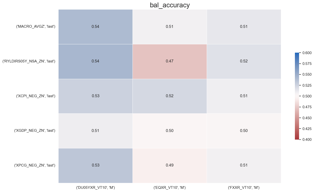
The single_statistic_table() function shows a table and heatmap for one chosen metric across all signal-return pairs.

Darker shades in the heatmap indicate stronger or more positive values.

srr.single_statistic_table(stat="bal_accuracy", 
                           show_heatmap=True, 
                           min_color= 0.4, 
                           max_color = 0.6, 
                           title_fontsize=20,
                           round=2
                           )

	Return	DU05YXR_VT10	EQXR_VT10	FXXR_VT10
	Frequency	M	M	M
Signal	Aggregation
MACRO_AVGZ	last	0.540963	0.507256	0.512603
RYLDIRS05Y_NSA_ZN	last	0.543418	0.472620	0.516887
XCPI_NEG_ZN	last	0.526198	0.522384	0.508718
XGDP_NEG_ZN	last	0.509713	0.500545	0.503055
XPCG_NEG_ZN	last	0.533591	0.493772	0.507683

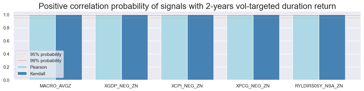
Correlation_bars

The correlation_bars() function plots correlation probabilities (Pearson and Kendall), and their significance, across signals, countries, or years.

You can segment bars by cross-section, calendar year, or signal to see where the relation is strongest or most reliable.

Important parameters:

• ret : target return category

• sigs : one signal, or a list of signals

• type : segmentation for the bars. i.e. "cross_section" (default), "years" , or "signals"

• freq : sampling frequency (e.g. "M" ), if you stored multiple

srr.correlation_bars(type="signals", 
                     size=(15, 3), 
                     title="Positive correlation probability of signals with 2-years vol-targeted duration return",
                     title_fontsize=20
                     )

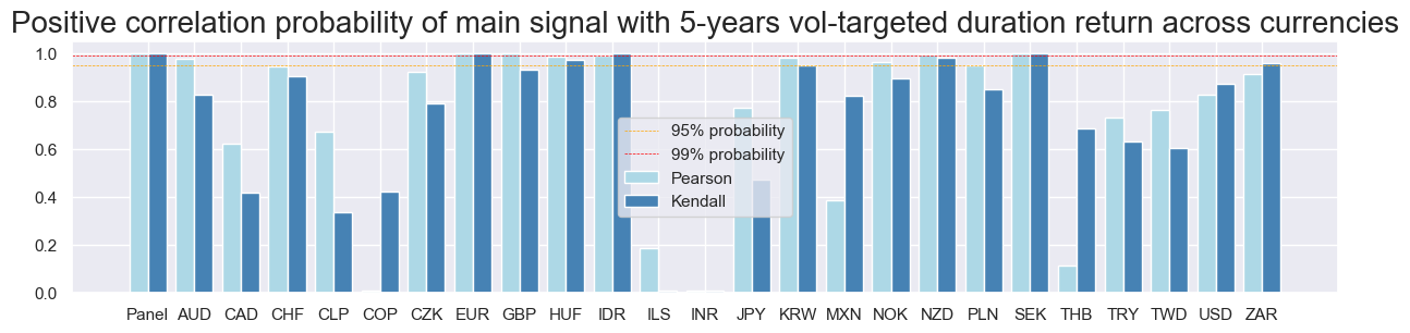
srr.correlation_bars(type="cross_section", 
                     title="Positive correlation probability of main signal with 5-years vol-targeted duration return across currencies", 
                     size=(15, 3),
                     title_fontsize=20)

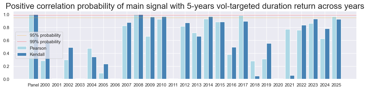
srr.correlation_bars(type="years", 
                     size=(15, 3), 
                     title="Positive correlation probability of main signal with 5-years vol-targeted duration return across years",
                     title_fontsize=20
                     )

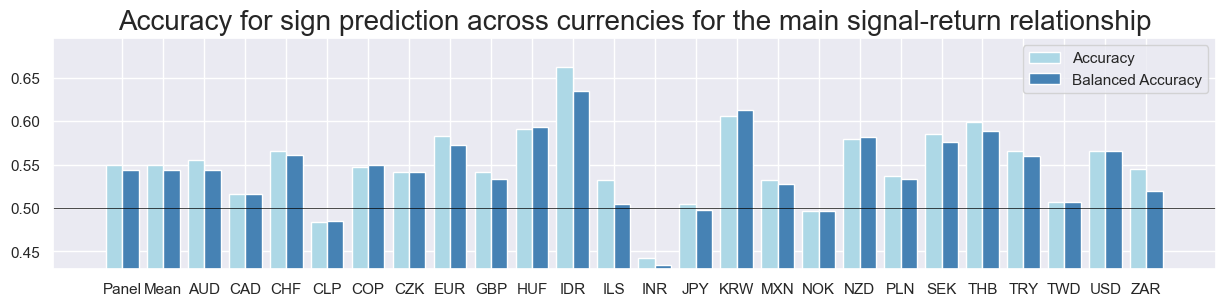
Accuracy_bars

The accuracy_bars() function works like correlation_bars() , but shows accuracy and balanced accuracy instead.

srr.accuracy_bars(type="cross_section", 
                  title="Accuracy for sign prediction across currencies for the main signal-return relationship", 
                  size=(15, 3),
                  title_fontsize=20
                  )

Backtesting

NaivePnL

The NaivePnl() class provides a quick and simple overview of a stylized PnL profile based on trading signals. It is called ‘naive’ because it deliberately ignores transaction costs and position constraints such as risk limits. These are excluded since costs and limitations depend on factors like trading size, institutional practices, and regulations.

Important parameters:

• ret : Return category.

• sigs : Signal categories.

• bms : List of benchmark tickers against which the correlations of PnL strategies are calculated and displayed.

• blacklist : Cross-sections with date ranges to exclude.

sigs = ["MACRO_AVGZ", "XGDP_NEG_ZN", "XCPI_NEG_ZN", "XPCG_NEG_ZN", "RYLDIRS05Y_NSA_ZN"]
    

naive_pnl = msn.NaivePnL(
    dfx,
    ret="DU05YXR_VT10",
    sigs=sigs,
    cids=cids,
    start="2004-01-01",
    blacklist=fxblack,
    bms=["USD_DU05YXR_NSA"],
)

make_pnl

The make_pnl() function calculates the daily PnL for a chosen signal category and appends it to the class instance’s main DataFrame. A single signal category can generate many different PnL series, depending on how the signal is transformed or specified in its final form.

Important parameters:

• sig : The signal category you want to turn into a PnL.

• sig_op : Signal transformation. Options:

  • zn_score_pan (default): Panel z-score: normalize across the whole cross-section.

  • zn_score_cs : Cross-sectional z-score: normalize within a smaller group or per-asset time series.

  • binary : Reduces the signal to +1/-1 positions (long or short).

  • raw : No transformation.

• rebal_freq : How often positions are rebalanced according to the signal. Options are 'daily' (default), 'weekly' , or 'monthly' . At each rebalancing date, only the signal value on that date is used to set positions. If make_zn_scores() is chosen as the method to produce raw signals, this same rebalancing frequency is also applied there.

• rebal_slip : Slippage (delay) in days for rebalancing. Default is 1 .

• thresh : Cutoff value for capping scores at a specified threshold,the maximum absolute score the function can output. The minimum allowed threshold is one standard deviation. By default, no threshold is applied.

• leverage : Multiplies the raw PnL series by a constant factor. This is a mechanical scaling, it does not change the time-varying riskiness of the strategy, only its overall level.

• vol_scale : Normalizes the strategy’s risk to a target volatility. The function estimates realized volatility over an expanding or rolling window and then scales positions so that the annualized volatility matches the chosen level. This creates a risk-managed PnL, where exposure shrinks during high-vol regimes and expands during low-vol regimes

i.e. Use leverage when you want a simple fixed rescaling of PnL and use vol_scale when you want dynamic adjustment to volatility.

for sig in sigs:
    naive_pnl.make_pnl(
        sig,
        sig_neg=False,
        sig_op="zn_score_pan",
        rebal_freq="monthly",
        vol_scale=10,
        rebal_slip=1,
        thresh=2,
        pnl_name=sig + "_NEGPZN"
    )

for sig in sigs:
    naive_pnl.make_pnl(
        sig,
        sig_neg=False,
        sig_op="binary",
        rebal_freq="monthly",
        vol_scale=10,
        rebal_slip=1,
        thresh=2,
        pnl_name=sig + "_NEGBN")

make_long_pnl

The make_long_pnl() function generates a daily long-only PnL by assuming equal long positions across all markets and time. This acts as a simple benchmark, providing a baseline to compare against signal-driven PnLs.

The vol_scale parameter adjusts the PnL to match a chosen annualized volatility level. This makes it easier to compare strategies by putting returns on a common risk scale, helping assess performance relative to volatility.

naive_pnl.make_long_pnl(vol_scale=10, label="Long_Only")

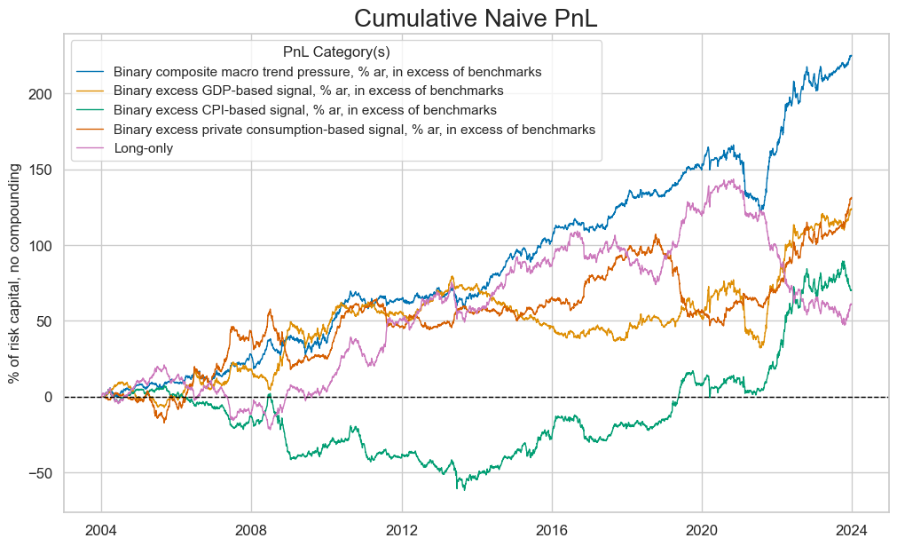
plot_pnls

Available naive PnLs can be listed with the pnl_names attribute:

The plot_pnls() function plots cumulative PnL as a line chart. It can show one or multiple PnL types across one or more cross-sections.

dict_labels = {"MACRO_AVGZ_NEGBN":  "Binary composite macro trend pressure, % ar, in excess of benchmarks", 
                "Long_Only": "Long-only",
                "XGDP_NEG_ZN_NEGBN": "Binary excess GDP-based signal, % ar, in excess of benchmarks", 
                "XCPI_NEG_ZN_NEGBN": "Binary excess CPI-based signal, % ar, in excess of benchmarks", 
                "XPCG_NEG_ZN_NEGBN": "Binary excess private consumption-based signal, % ar, in excess of benchmarks"
               }


naive_pnl.plot_pnls(
    pnl_cats=[
        "MACRO_AVGZ_NEGBN",
        "XGDP_NEG_ZN_NEGBN",
        "XCPI_NEG_ZN_NEGBN", 
        "XPCG_NEG_ZN_NEGBN",
        "Long_Only",
    ],
    xcat_labels=dict_labels,
    pnl_cids=["ALL"],
    start="2004-01-01",
    end="2023-12-31",
    title_fontsize=20
)

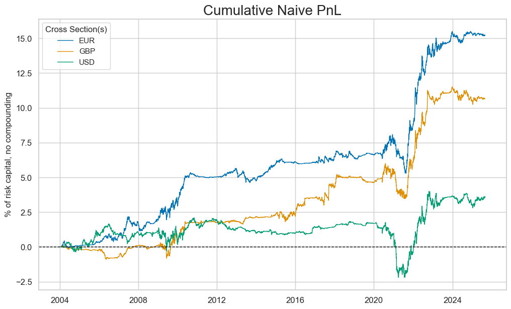
cidx = ["EUR", "GBP", "USD"]

naive_pnl.plot_pnls(
    pnl_cats=["MACRO_AVGZ_NEGPZN"],
    pnl_cids=cidx,
    title_fontsize=20,
    start="2004-01-01",
   # end="2021-01-01",
)

evaluate_pnls

The evaluate_pnls() function returns a small dataframe of key PnL statistics. For definitions of Sharpe and Sortino ratios, please see here

The table can only have multiple PnL categories or multiple cross-sections, not both at the same time. The table also shows the daily benchmark correlation of PnLs.

df_eval = naive_pnl.evaluate_pnls(
    pnl_cats=["MACRO_AVGZ_NEGBN", "XPCG_NEG_ZN_NEGBN", ], pnl_cids=["ALL"], start="2004-01-01", end="2023-12-01"
)

display(df_eval.astype("float").round(2))

xcat	MACRO_AVGZ_NEGBN	XPCG_NEG_ZN_NEGBN
Return %	11.13	6.30
St. Dev. %	9.61	9.68
Sharpe Ratio	1.16	0.65
Sortino Ratio	1.69	0.97
Max 21-Day Draw %	-22.17	-16.95
Max 6-Month Draw %	-34.91	-40.03
Peak to Trough Draw %	-44.13	-60.53
Top 5% Monthly PnL Share	0.56	0.92
USD_DU05YXR_NSA correl	-0.02	-0.37
Traded Months	240.00	240.00

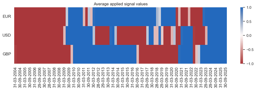
signal_heatmap

The signal_heatmap() function shows a heatmap of signal values over time and cross-sections for a specific strategy.

naive_pnl.signal_heatmap(
    pnl_name="XPCG_NEG_ZN_NEGBN",
    pnl_cids=["EUR", "USD", "GBP"],
    freq="q",
    start="2004-01-01",
)

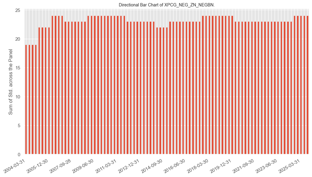
agg_signal_bars

The agg_signal_bars() function shows the size and direction of the aggregate signal over time.

naive_pnl.agg_signal_bars(
    pnl_name="XPCG_NEG_ZN_NEGBN",
    freq="q",
    metric="direction",
)

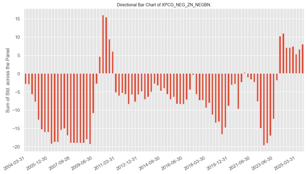
naive_pnl.agg_signal_bars(
    pnl_name="XPCG_NEG_ZN_NEGBN",
    freq="q",
    metric="strength",
)