Commodity future returns #
This category group contains daily USD-denominated commodity future returns. These returns are based on positions in the front contract of the most liquid available future of each type of commodity.
Commodity future returns in % of notional #
Ticker : COXR_NSA
Label : Commodity future return, % of notional.
Definition : Return on the front future of the specified commodity contract, % of the notional of the contract.
Notes :
-
The return is the % change in the futures price. The return calculation assumes the future position is rolled (from front to second) on the first day of the month when the contract is deliverable.
-
For futures return calculations, the following groups of commodity contracts have been used: energy, base metals, precious metals, agricultural commodities and livestock.
-
For information on the components comprising each commodity group, see Appendix 1 .
Vol-targeted commodity future return #
Ticker : COXR_VT10
Label : Commodity future return for 10% vol target.
Definition : Return on the front future of the specified commodity contract, % of risk capital on position scaled to 10% (annualized) volatility target.
Notes :
-
Positions are scaled to a 10% volatility target based on the historic standard deviation for an exponential moving average with a half-life of 11 days. Positions are rebalanced at the end of each month.
-
See further the related notes above on “Commodity return in % of notional” (
COXR_NSA). -
For information on the components comprising each commodity group, see Appendix 1 .
Imports #
Only the standard Python data science packages and the specialized
macrosynergy
package are needed.
import os
import numpy as np
import pandas as pd
import matplotlib.pyplot as plt
import seaborn as sns
import math

import json
import yaml

import macrosynergy.management as msm
import macrosynergy.panel as msp
import macrosynergy.signal as mss
import macrosynergy.pnl as msn


from macrosynergy.download import JPMaQSDownload

from timeit import default_timer as timer
from datetime import timedelta, date, datetime

import warnings

warnings.simplefilter("ignore")
The
JPMaQS
indicators we consider are downloaded using the J.P. Morgan Dataquery API interface within the
macrosynergy
package. This is done by specifying
ticker strings
, formed by appending an indicator category code
<category>
to a currency area code
<cross_section>
. These constitute the main part of a full quantamental indicator ticker, taking the form
DB(JPMAQS,<cross_section>_<category>,<info>)
, where
<info>
denotes the time series of information for the given cross-section and category. The following types of information are available:
-
valuegiving the latest available values for the indicator -
eop_lagreferring to days elapsed since the end of the observation period -
mop_lagreferring to the number of days elapsed since the mean observation period -
gradedenoting a grade of the observation, giving a metric of real time information quality.
After instantiating the
JPMaQSDownload
class within the
macrosynergy.download
module, one can use the
download(tickers,start_date,metrics)
method to easily download the necessary data, where
tickers
is an array of ticker strings,
start_date
is the first collection date to be considered and
metrics
is an array comprising the times series information to be downloaded.
# Define cross sections (currency tickers)
cids_dmca = [
    "AUD",
    "CAD",
    "CHF",
    "EUR",
    "GBP",
    "JPY",
    "NOK",
    "NZD",
    "SEK",
    "USD",
]  # DM currency areas
cids_dmec = ["DEM", "ESP", "FRF", "ITL", "NLG"]  # DM euro area countries
cids_latm = ["BRL", "COP", "CLP", "MXN", "PEN"]  # Latam countries
cids_emea = ["CZK", "HUF", "ILS", "PLN", "RON", "RUB", "TRY", "ZAR"]  # EMEA countries
cids_emas = [
    "CNY",
    "IDR",
    "INR",
    "KRW",
    "MYR",
    "PHP",
    "SGD",
    "THB",
    "TWD",
]


cids_dm = cids_dmca + cids_dmec
cids_em = cids_latm + cids_emea + cids_emas

cids_eco = sorted(cids_dm + cids_em)


cids_nfm = ["GLD", "SIV", "PAL", "PLT"]
cids_fme = ["ALM", "CPR", "LED", "NIC", "TIN", "ZNC","SIO","SRR"]
cids_ene = ["BRT", "WTI", "NGS", "GSO", "HOL","EUA"]
cids_sta = ["COR", "WHT", "SOY", "CTN","SOO","SOM","KKW","CAO"]
cids_liv = ["CAT", "HOG","CFD"]
cids_mis = ["CFE", "SGR", "NJO", "CLB","CAO"]
cids = cids_nfm + cids_fme + cids_ene + cids_sta + cids_liv + cids_mis
# Define quantamental indicators (category tickers)

main = ["COXR_NSA", "COXR_VT10"]
econ = ["IVAWGT_SA_1YMA", "IVAWGT_SA_3YMA"]
mark = [
    "MBCSCORE_SA_D3M3ML3",
    "MBCSCORE_SA_3MMA",
    "MBCSCORE_SA_D1M1ML12",
    "MBOSCORE_SA_D3M3ML3",
    "MBOSCORE_SA_3MMA",
    "MBOSCORE_SA_D1M1ML12",
    "MBISCORE_SA_D3M3ML3",
    "MBISCORE_SA_3MMA",
    "MBISCORE_SA_D1M1ML12",
    "CBCSCORE_SA_D3M3ML3",
    "CBCSCORE_SA_3MMA",
    "CBCSCORE_SA_D1M1ML12",
    "CBOSCORE_SA_D3M3ML3",
    "CBOSCORE_SA_3MMA",
    "CBOSCORE_SA_D1M1ML12",
    "CBISCORE_SA_D3M3ML3",
    "CBISCORE_SA_3MMA",
    "CBISCORE_SA_D1M1ML12",
]
xcats = main + econ + mark
# Download series from J.P. Morgan DataQuery by tickers

start_date = "1990-01-01"
tickers = [cid + "_" + xcat for cid in cids + cids_eco for xcat in xcats]
print(f"Maximum number of tickers is {len(tickers)}")

# Retrieve credentials

client_id: str = os.getenv("DQ_CLIENT_ID")
client_secret: str = os.getenv("DQ_CLIENT_SECRET")

# Download from DataQuery

with JPMaQSDownload(client_id=client_id, client_secret=client_secret) as downloader:
    start = timer()
    assert downloader.check_connection()
    df = downloader.download(
        tickers=tickers,
        start_date=start_date,
        metrics=["value", "eop_lag", "mop_lag", "grading"],
        suppress_warning=True,
        show_progress=True,
    )
    end = timer()

dfd = df

print("Download time from DQ: " + str(timedelta(seconds=end - start)))
Maximum number of tickers is 1562
Downloading data from JPMaQS.
Timestamp UTC:  2025-08-04 16:39:06
Connection successful!
Requesting data: 100%|███████████████████████████████████████████████████████████████| 308/308 [01:15<00:00,  4.10it/s]
Downloading data: 100%|██████████████████████████████████████████████████████████████| 308/308 [00:20<00:00, 14.95it/s]
Some expressions are missing from the downloaded data. Check logger output for complete list.
4440 out of 6160 expressions are missing. To download the catalogue of all available expressions and filter the unavailable expressions, set `get_catalogue=True` in the call to `JPMaQSDownload.download()`.
Download time from DQ: 0:01:50.599189
Availability #
cids_exp = cids
msm.missing_in_df(dfd, xcats=main, cids=cids_exp)
No missing XCATs across DataFrame.
Missing cids for COXR_NSA:   []
Missing cids for COXR_VT10:  []
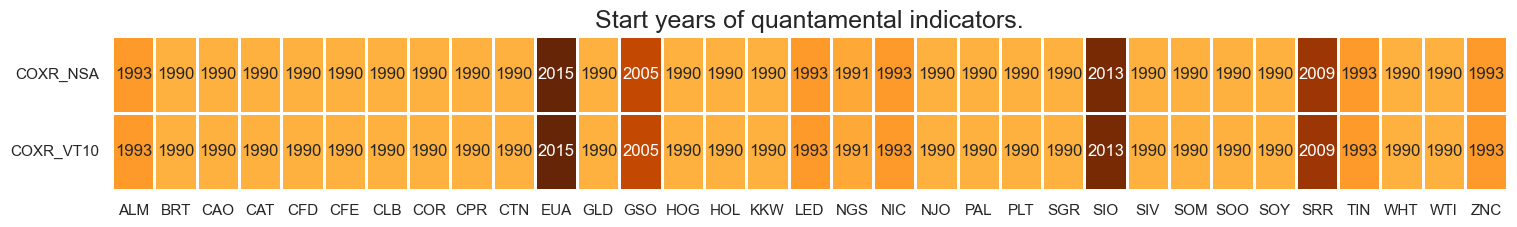
The vast majority of commodity futures return series’ are available by 2000. Heating oil is the notable late-starter, only available from 2007 onwards.
For the explanation of commodity symbols, please view Appendix 1 .
xcatx = main
cidx = cids_exp

dfx = msm.reduce_df(dfd, xcats=xcatx, cids=cidx)
dfs = msm.check_startyears(
    dfx,
)
msm.visual_paneldates(dfs, size=(18, 2))

print("Last updated:", date.today())
Last updated: 2025-08-04
History #
Commodity future returns in % of notional #
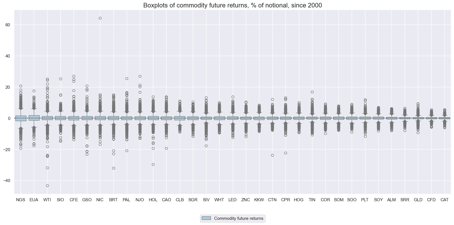
Daily returns have displayed modest differences in variations across commodities and a general proclivity to occasional outliers on both the negative and positive side. Natural gas has seen the greatest daily volatility, whilst aluminium, gold and cattle have been subject to the least.
Note: On April 20th 2020, during the COVID pandemic-related market turmoil, the front future price for WTI crude collapsed to a recorded -37 dollars from over 18 dollars, marking a loss of almost 300%. Since negative prices are not valid for standard return calculations, we have replaced the value by the average of the two surrounding days.
xcatx = ["COXR_NSA"]
cidx = cids_exp

msp.view_ranges(
    dfd,
    xcats=xcatx,
    cids=cidx,
    sort_cids_by="std",
    start=start_date,
    kind="box",
    title="Boxplots of commodity future returns, % of notional, since 2000",
    xcat_labels=["Commodity future returns"],
    size=(16, 8),
)
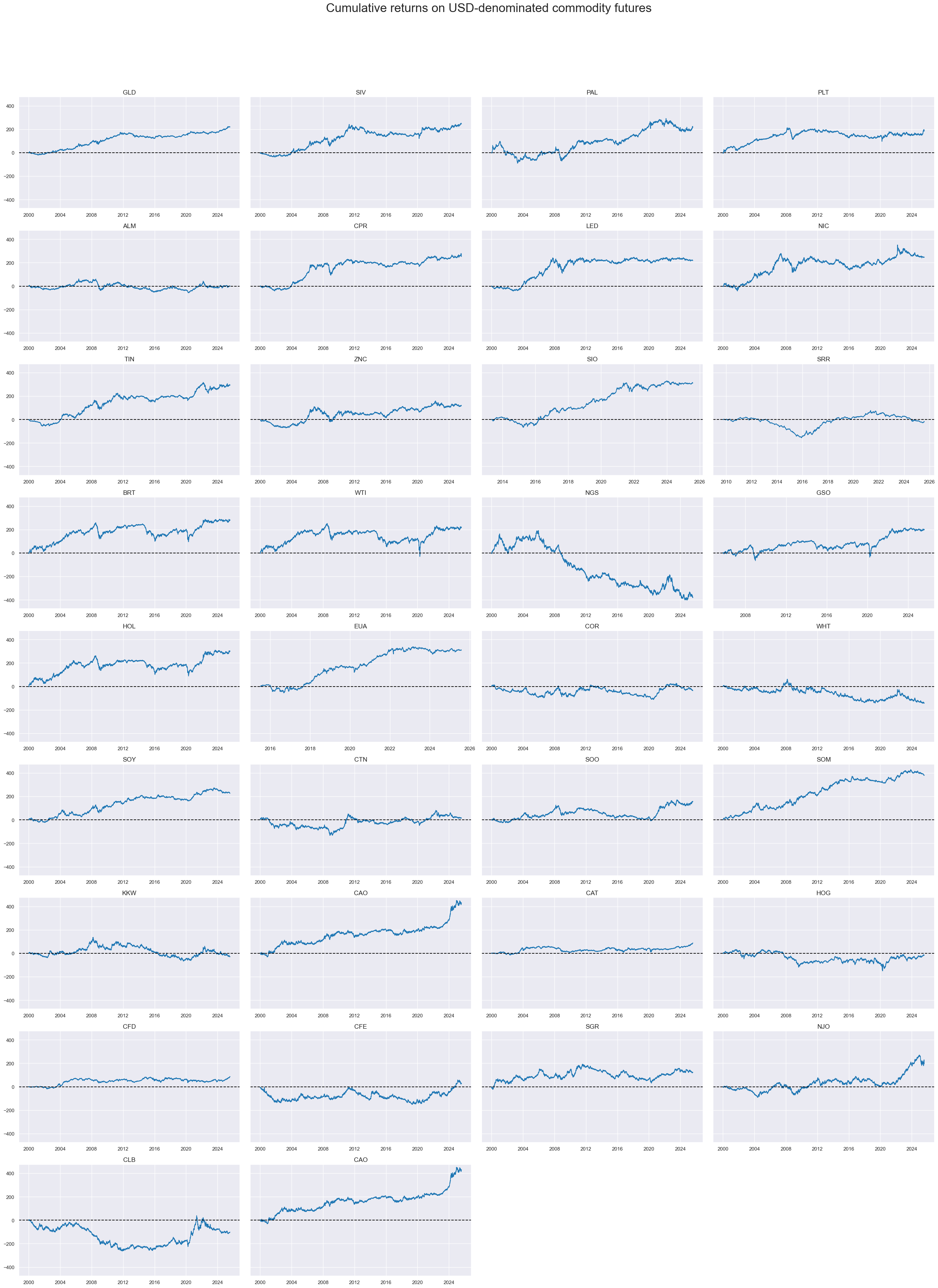
Long-term performance (since 2000) has been vastly different across commodities. Crude, Nickel, Palladium, Silver and Soy produced near 300% cumulative return, while aluminum, coffee and wheat recorded small negative returns.
xcatx = ["COXR_NSA"]
cidx = cids_exp

msp.view_timelines(
    dfd,
    xcats=xcatx,
    cids=cidx,
    start="2000-01-01",
    title="Cumulative returns on USD-denominated commodity futures",
    title_fontsize=27,
    legend_fontsize=17,
    cumsum=True,
    title_adj=1.03,
    title_xadj=0.52,
    ncol=4,
    same_y=True,
    size=(12, 7),
    aspect=1.7,
    all_xticks=True,
)
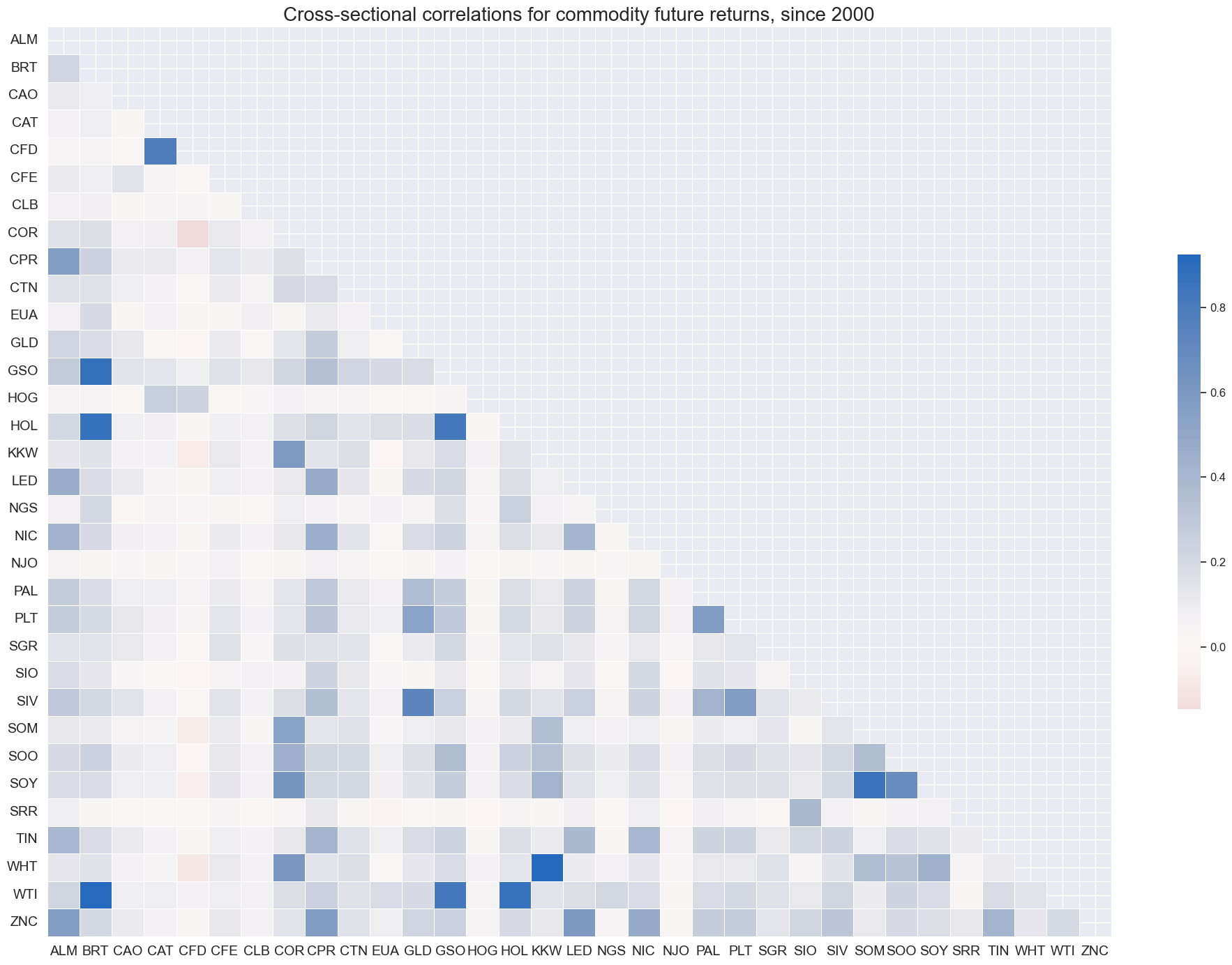
Despite the vast long-term return differences, short-term commodity returns have been mostly positively correlated. Cattle, hogs, lumber, natural gas, and orange juice have been the most idiosyncratic contracts.
xcatx = "COXR_NSA"
cidx = cids_exp

msp.correl_matrix(
    dfd,
    xcats=xcatx,
    cids=cidx,
    title="Cross-sectional correlations for commodity future returns, since 2000",
    size=(20, 14),
)
Vol-targeted commodity future returns #
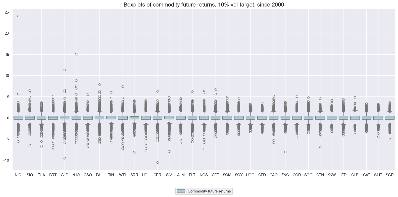
Volatility targeting (on a monthly basis) can be perilous in the commodity space and produced some spectacular daily return outliers for targeted posititions, particularly in nickel, cotton, live cattle, gold and silver.
xcatx = ["COXR_VT10"]
cidx = cids_exp

msp.view_ranges(
    dfd,
    xcats=xcatx,
    cids=cidx,
    sort_cids_by="std",
    start=start_date,
    kind="box",
    title="Boxplots of commodity future returns, 10% vol-target, since 2000",
    xcat_labels=["Commodity future returns"],
    size=(16, 8),
)
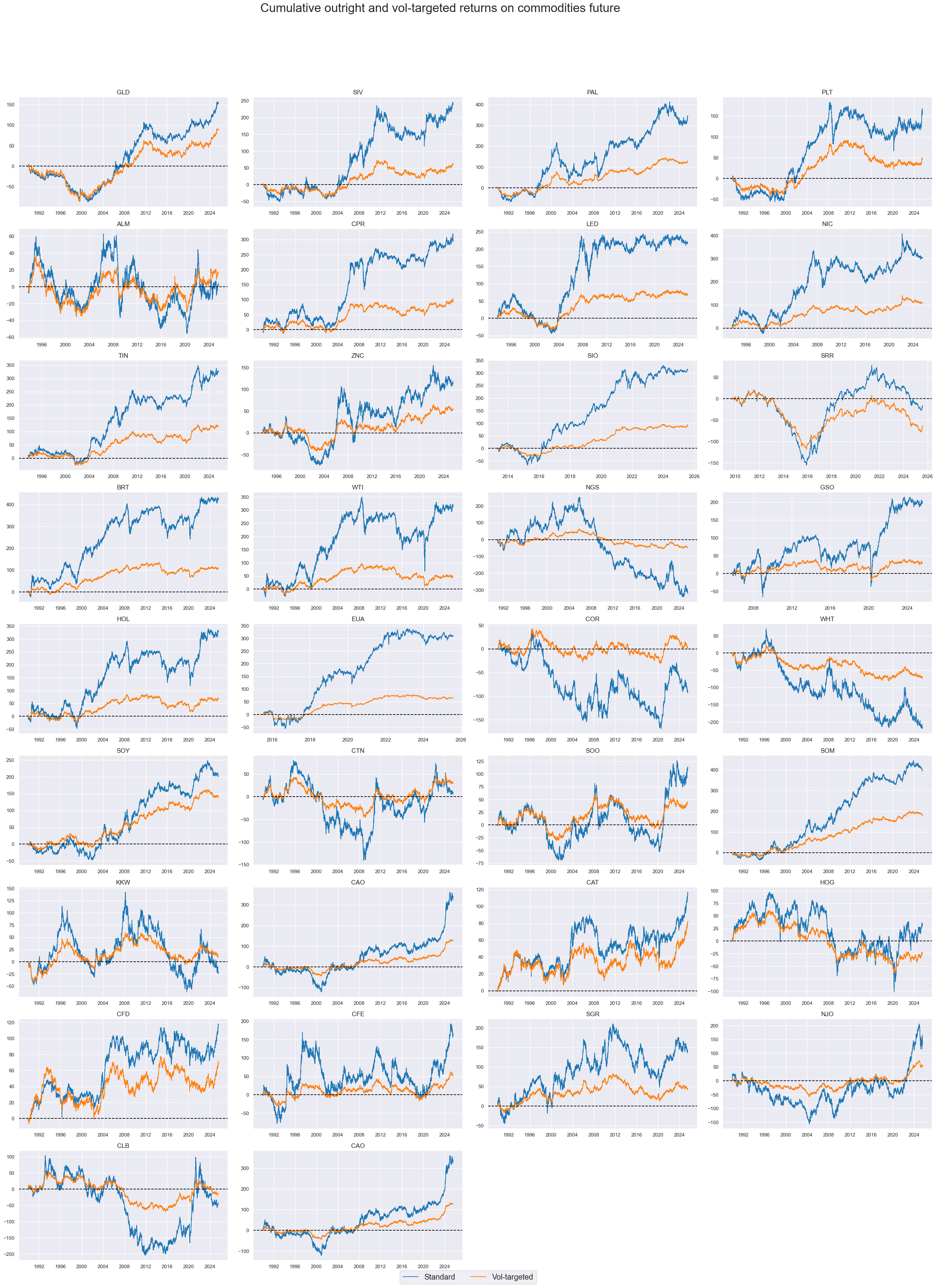
Volatility targeting makes a big difference in the long-term return performance. On a notional basis, the return differential between Brent and aluminum has been close to 200%, whilst on a vol-targeted basis, it was less than 30%.
xcatx = ["COXR_NSA", "COXR_VT10"]
cidx = cids_exp

msp.view_timelines(
    dfd,
    xcats=xcatx,
    cids=cidx,
    start=start_date,
    title="Cumulative outright and vol-targeted returns on commodities future",
    xcat_labels=["Standard", "Vol-targeted"],
    title_fontsize=27,
    legend_fontsize=17,
    title_adj=1.03,
    title_xadj=0.47,
    cumsum=True,
    ncol=4,
    same_y=False,
    size=(12, 7),
    aspect=1.7,
    all_xticks=True,
)
Importance #
Research links #
“Herding Behaviour in Commodity Markets…Broad basket commodities and energy-based ETFs are generally susceptible to herding across most frequencies…Agricultural and metal-based ETFs are least prone to herding in general.” Mand, Sifat, Ang and Choo
“We estimate the skewness of the unconditional distribution of energy returns (over past decades) and test its statistical significance…Our results show that crude oil (Brent and WTI) and Gasoline returns are negatively skewed while other energy returns such as Heating oil, Kerosene and Natural gas seem to be symmetrically distributed. This indicates that the returns of the former are likely to encapsulate more largely the effect of negative shocks and so present higher tail risk than those of the latter.” Carnero, Leon, and Niguez
“We estimate the skewness of the unconditional distribution of energy returns (over past decades) and test its statistical significance…Our results show that crude oil (Brent and WTI) and Gasoline returns are negatively skewed while other energy returns such as Heating oil, Kerosene and Natural gas seem to be symmetrically distributed. This indicates that the returns of the former are likely to encapsulate more largely the effect of negative shocks and so present higher tail risk than those of the latter.” Carnero, Leon, and Niguez
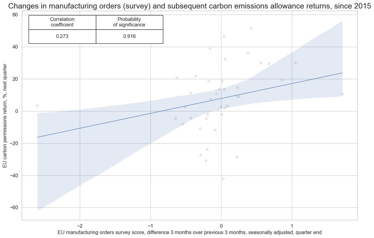
Empirical clues #
Although data on carbon emissions returns have only been available since 2015, there is increasingly significant evidence that they can be predicted by changes in the EU manufacturing orders survey score. Rising manufacturing orders require higher production and more emissions in the short term.
lc_xcats = [
    "MBCSCORE_SA_D3M3ML3",
    "MBCSCORE_SA_3MMA",
    "MBCSCORE_SA_D1M1ML12",
    "MBOSCORE_SA_D3M3ML3",
    "MBOSCORE_SA_3MMA",
    "MBOSCORE_SA_D1M1ML12",
    "MBISCORE_SA_D3M3ML3",
    "MBISCORE_SA_3MMA",
    "MBISCORE_SA_D1M1ML12",
]
# creating the linear composite for each of the Manufacturing categories
for xc in lc_xcats:
    dfa = msp.linear_composite(
        df=dfd,
        xcats=xc,
        cids=["CZK", "HUF",  "PLN", "RON", "EUR"] ,
        weights="IVAWGT_SA_1YMA",
        new_cid="EUA",
        complete_cids=False,
    )
    dfd = msm.update_df(dfd, dfa)
dfa = dfd[dfd["cid"]=="EUA"]
dfa["xcat"]  = "EUR" + dfa["xcat"]
dfa["cid"] = "EUR"
dfd = msm.update_df(dfd, dfa)
cr = msp.CategoryRelations(
    dfd,
    xcats=["MBOSCORE_SA_D3M3ML3", "COXR_NSA"],
    cids=["EUA"],
    freq="Q",
    lag=1,
    xcat_aggs=["last", "sum"],
    fwin=1,
    start="2000-01-01",
    years=None,
)

cr.reg_scatter(
    title="Changes in manufacturing orders (survey) and subsequent carbon emissions allowance returns, since 2015",
    title_fontsize=18,
    labels=False,
    coef_box="upper left",
    xlab="EU manufacturing orders survey score, difference 3 months over previous 3 months, seasonally adjusted, quarter end",
    ylab="EU carbon permissions return, %, next quarter",
    prob_est="pool",
    size=(12, 8),
)
Appendices #
Appendix 1: Commodity group definitions and symbols #
The commodity groups considered are: energy, base metals, precious metals, agricultural commodities and livestock.
-
The energy commodity group contains:
-
BRT : ICE Brent crude (IPE Brent crude before 2003), futures contracts for Brent crude oil sourced from the North Sea traded on the intercontinetal exchange (ICE).
-
WTI : NYMEX WTI light crude, futures contracts for West Texas Intermediate (WTI) crude, primarily sourced from Texas and surronding states, traded on the New York Mercantile Exchange (NYMEX).
-
NGS : NYMEX natural gas, Henry Hub, the global benchmark for natural gas pricing in North America based on delivery at the Henry Hub in Louisiana, traded on the New York Mercantile Exchange (NYMEX).
-
GSO : NYMEX RBOB Gasoline, futures contracts for Reformulated Gasoline Blendstock for Oxygenate Blending, the primary benchmark for wholesale U.S. gasoline prices, traded on the New York Mercantile Exchange (NYMEX).
-
HOL : NYMEX Heating oil, New York Harbor ULSD, futures contracts for ultra-low sulfur distillate fuel oil, traded on the New York Mercantile Exchange (NYMEX).
-
EUA : EEX EU Allowance; a carbon permit traded on the European Energy Exchange (EEX).
-
-
The base metals group contains:
-
ALM : London Metal Exchange aluminium, is the standardized aluminium futures contract traded on the London Metal Exchange (LME).
-
CPR : Comex copper, is the standardized copper futures contract traded on the Commodity Exchange (COMEX).
-
LED : London Metal Exchange Lead, is the standardized lead futures contract traded on the London Metal Exchange (LME).
-
NIC : London Metal Exchange Nickel, is the standardized nickel futures contract traded on the London Metal Exchange (LME).
-
TIN : London Metal Exchange Tin, is the standardized tin futures contract traded on the London Metal Exchange (LME).
-
ZNC : London Metal Exchange Zinc, is the standardized zinc futures contract traded on the London Metal Exchange (LME).
-
SIO : SGX TSI Iron ore CFR, the world’s primary benchmark for seaborne iron ore prices sent to China mainly, traded on the Singapore Exchange (SGX).
-
SRR : Shanghai Futures Exchange Steel Rebar, the primary benchmark for rebar pricing in China traded on the Shanghai Futures Exchange (SHFE).
-
-
The precious metals group contains:
-
GLD : COMEX gold 100 Ounce, futures contract for gold traded on the Commodity Exchange (COMEX), one of the primary benchmarks for gold, trading 100 troy ounces of gold.
-
SIV : COMEX silver 5000 Ounce, futures contract for silver traded on the Commodity Exchange (COMEX), one of the primary benchmarks for silver, trading 5000 troy ounces of silver.
-
PAL : NYMEX palladium, futures contract for palladium traded on the New York metal exchange (NYMEX), one of the primary benchmarks for palladium.
-
PLT : NYMEX platinum, futures contract for platinum traded on the New York metal exchange (NYMEX), one of the primary benchmarks for platinum.
-
-
The agricultural commodity group contains:
-
COR : Chicago Board of Trade corn composite, the global benchmark futures contract for trading corn on the Chicago Board of Trade (CBOT).
-
WHT : Chicago Board of Trade wheat composite, the global benchmark futures contract for trading soft red winter wheat on the Chicago Board of Trade (CBOT).
-
SOY : Chicago Board of Trade soybeans composite, the global benchmark futures contract for trading soybeans on the Chicago Board of Trade (CBOT).
-
SOO : Chicago Board of Trade soybean oil composite, the global benchmark futures contract for trading soybean meal on the Chicago Board of Trade (CBOT).
-
SOM : Chicago Board of Trade soybean meal composite, the global benchmark futures contract for trading soybean oil, used for animal feed, on the Chicago Board of Trade (CBOT).
-
CTN : NYBOT / ICE cotton #2, the global benchmark futures contract for trading raw cotton, traded on the Intercontinental Exchange (ICE).
-
CFE : NYBOT / ICE coffee ‘C’ Arabica, the global benchmark futures contract for trading arabica coffee beans, traded on the Intercontinental Exchange (ICE).
-
SGR : NYBOT / ICE raw cane sugar #11, the global benchmark futures contract for trading raw cane sugar, traded on the Intercontinental Exchange (ICE).
-
NJO : NYBOT / NYCE FCOJ frozen orange juice concentrate, the global benchmark for global orange juice prices, traded on the Chicago Mercantile Exchange (CME).
-
CLB : Chicago Mercantile Exchange random length lumber, a key benchmark for softwood lumber prices from North America, traded on the Chicago Mercantile Exchange (CME).
-
KKW : Kansas City Board of Trade HRW Wheat composite, benchmark price for futures of hard red winter wheat grown primarily in the Great Plains (Kansas, Oklahoma, Texas, Colorado, Nebraska), traded on the Chicago Mercantile Exchange (CME).
-
CAO : ICE Cocoa, the global benchmark futures contract for trading raw cocoa beans, traded on the Intercontinental Exchange (ICE).
-
-
The (U.S.) livestock commodity group contains:
-
CAT : Chicago Mercantile Exchange live cattle composite, primary benchmark for trading live-fed cattle traded on the Chicago Mercantile Exchange (CME).
-
HOG : Chicago Mercantile Exchange lean hogs composite, primary benchmark for trading hogs ready for slaughter traded on the Chicago Mercantile Exchange (CME).
-
CFD : Chicago Mercantile Exchange feeder cattle composite, primary benchmark for trading young lightweight cattle entering US feedlots traded on the Chicago Mercantile Exchange (CME).
-