Economic surprises and commodity futures returns #
Get packages and JPMaQS data #
Import and setup #
This notebook uses standard packages from the Python data science stack, plus the specialised
macrosynergy
package, which streamlines workflows in two key areas:
-
JPMaQS data download : Simplifies access to macro-quantamental indicators via the JPMorgan DataQuery REST API, handling formatting and filtering with minimal code.
-
Analysing quantamental signals : Accelerates analysis of macro trading signals, with built-in tools for normalisation, charting, and performance attribution.
For full documentation, see our Introduction to the Macrosynergy package or the Kaggle notebook . Technical reference documentation of the package is available on GitHub .
Installation:
pip install macrosynergy --upgrade
Credentials: Set your JPMorgan DataQuery credentials either directly in code or as environment variables:
DQ_CLIENT_ID: str = "your_client_id"
DQ_CLIENT_SECRET: str = "your_client_secret"
Corporate users behind firewalls can configure proxy settings via the PROXY = {} variable ( example here ).
# Constants and credentials
import os

REQUIRED_VERSION: str = "1.2.2"
DQ_CLIENT_ID: str = os.getenv("DQ_CLIENT_ID")
DQ_CLIENT_SECRET: str = os.getenv("DQ_CLIENT_SECRET")
PROXY = {}  # Configure if behind corporate firewall
START_DATE: str = "1990-01-01"
import macrosynergy as msy

msy.check_package_version(required_version=REQUIRED_VERSION)
# If version check fails: pip install macrosynergy --upgrade
if not DQ_CLIENT_ID or not DQ_CLIENT_SECRET:
    raise ValueError(
        "Missing DataQuery credentials. Please set DQ_CLIENT_ID and DQ_CLIENT_SECRET as environment variables or insert them directly in the notebook."
    )
# Standard imports
import numpy as np
import pandas as pd
import matplotlib.pyplot as plt
import seaborn as sns
from typing import Dict, List, Tuple
import warnings

# Macrosynergy package
import macrosynergy.management as msm
import macrosynergy.panel as msp
import macrosynergy.pnl as msn
import macrosynergy.signal as mss
import macrosynergy.visuals as msv
from macrosynergy.download import JPMaQSDownload
We download macro-quantamental indicators from JPMaQS using the J.P. Morgan DataQuery API via the
macrosynergy
package.
DataQuery expressions follow the structure:
DB(JPMAQS,<cross_section>_<category>,<info>)
, where:
-
JPMAQS: the dataset name -
<cross_section>_<category>: the JPMaQS ticker (e.g.,USD_EQXR01XD) -
<info>: time series type
Common
<info>
attributes include:
-
value: latest available indicator value -
eop_lag: days since end of observation period -
mop_lag: days since mean observation period -
grade: real-time quality metric -
last_updated: timestamp of the last update for the time series
This notebook uses
value
and
eop_lag
attributes.
The
JPMaQSDownload
class takes a list of JPMaQS tickers (
<cross_section>_<category>
format) via
              .download(tickers,


              start_date,


              metrics)
and handles the DataQuery expression construction, throttle limits, and parallel data requests automatically.
Data selection and download #
# Currency area groupings for macro analysis
cids_dmca: List[str] = [
    "AUD", "CAD", "CHF", "EUR", "GBP",
    "JPY", "NOK", "NZD", "SEK", "USD"
]  # Developed market currency areas

cids_latm: List[str] = ["BRL", "COP", "CLP", "MXN", "PEN"]  # Latin America
cids_emea: List[str] = ["CZK", "HUF", "ILS", "PLN", "RON", "RUB", "TRY", "ZAR"]  # EMEA
cids_emas: List[str] = ["CNY", "IDR", "INR", "KRW", "MYR", "PHP", "SGD", "THB", "TWD"]  # EM Asia

# Aggregate currency groupings
cids_dm: List[str] = cids_dmca
cids_em: List[str] = cids_latm + cids_emea + cids_emas
cids: List[str] = sorted(cids_dm + cids_em)

# Commodity-sensitive FX
cids_cofx: List[str] = ["AUD", "BRL", "CAD", "CLP", "NZD", "PEN", "RUB"]

# Commodity cross-sections by sector
cids_bams: List[str] = ["ALM", "CPR", "LED", "NIC", "TIN", "ZNC"]  # Base metals
cids_prms: List[str] = ["PAL", "PLT"]  # Precious industrial metals
cids_fuen: List[str] = ["BRT", "WTI", "HOL", "GSO"]  # Energy
cids_gold: List[str] = ["GLD"]  # Gold

cids_coms: List[str] = cids_bams + cids_prms + cids_fuen  # Non-gold commodities
# Quantamental categories of interest

# Industrial production transformations
ip_monthly: List[str] = ["P3M3ML3AR", "P6M6ML6AR", "P1M1ML12_3MMA"]
ip_quarterly: List[str] = ["P1Q1QL1AR", "P2Q2QL2AR", "P1Q1QL4"]

# Generate all IP indicators (monthly + quarterly)
ips: List[str] = [
    f"IP_SA_{transform}_ARMAS"
    for transform in ip_monthly + ip_quarterly
]

# Confidence survey transformations
confidence_monthly: List[str] = [
    "_3MMA",
    "_D1M1ML1",
    "_D3M3ML3",
    "_D6M6ML6",
    "_3MMA_D1M1ML12",
    "_D1M1ML12",
]
confidence_quarterly: List[str] = ["_D1Q1QL1", "_D2Q2QL2", "_D1Q1QL4"]
confidence_transforms: List[str] = [""] + confidence_monthly + confidence_quarterly

# Manufacturing confidence (all transformations)
mcs: List[str] = [
    f"MBCSCORE_SA{transformation}_ARMAS"
    for transformation in confidence_transforms
]

# Construction confidence (all transformations)
ccs: List[str] = [
    f"CBCSCORE_SA{transformation}_ARMAS"
    for transformation in confidence_transforms
]

# Core analytical factors (primary signals)
main: List[str] = ips + mcs + ccs

# Economic context indicators
econ: List[str] = [
    "USDGDPWGT_SA_1YMA",  # USD-weighted GDP trends (1-year)
    "USDGDPWGT_SA_3YMA",  # USD-weighted GDP trends (3-year)
    "IVAWGT_SA_1YMA",     # Investment value-added weights
]

# Market context indicators
mark: List[str] = [
    "COXR_VT10",  # Commodity return, vol-targeted
    "EQXR_NSA",   # Equity index futures returns
    "EQXR_VT10",  # Equity index futures returns, vol-targeted
]

# Combine all categories
xcats: List[str] = main + econ + mark
For further documentation of the indicators used see the Macro Quantamental Academy or JPMorgan Markets (password protected):
# Construct list of JPMaQS tickers for download
tickers: List[str] = []

# Core analytical indicators for all cross-sections
tickers += [f"{cid}_{xcat}" for cid in cids for xcat in main]

# Economic context indicators for all cross-sections
tickers += [f"{cid}_{xcat}" for cid in cids for xcat in econ]

# Market context indicators with specific rules
for xcat in mark:
    if xcat.startswith("CO"):  # Commodity returns: use commodity cross-sections
        tickers += [f"{cid}_{xcat}" for cid in cids_coms + cids_gold]
    elif xcat.startswith("EQ"):  # Equity indicators: USD only (S&P 500)
        tickers += [f"USD_{xcat}"]
    else:
        raise NotImplementedError(f"Unknown category for mark: {xcat}")

print(f"Maximum number of JPMaQS tickers to be downloaded is {len(tickers)}")
Maximum number of JPMaQS tickers to be downloaded is 943
# Download macro-quantamental indicators from JPMaQS via the DataQuery API
with JPMaQSDownload(
    client_id=DQ_CLIENT_ID,
    client_secret=DQ_CLIENT_SECRET,
    proxy=PROXY
) as downloader:
    df: pd.DataFrame = downloader.download(
        tickers=tickers,
        start_date=START_DATE,
        metrics=["value", "eop_lag"],
        suppress_warning=True,
        show_progress=True,
        report_time_taken=True,
        get_catalogue=True,
    )
Downloading the JPMAQS catalogue from DataQuery...
Downloaded JPMAQS catalogue with 23201 tickers.
Removed 788/1886 expressions that are not in the JPMaQS catalogue.
Downloading data from JPMaQS.
Timestamp UTC:  2025-06-26 14:05:41
Connection successful!
Requesting data: 100%|█████████████████████████████████████████████████████████████████| 55/55 [00:11<00:00,  4.93it/s]
Downloading data: 100%|████████████████████████████████████████████████████████████████| 55/55 [00:38<00:00,  1.44it/s]
Time taken to download data: 55.63 seconds.
# Preserve original downloaded data for debugging and comparison

dfx = df.copy()
dfx.info()
<class 'pandas.core.frame.DataFrame'>
RangeIndex: 3790405 entries, 0 to 3790404
Data columns (total 5 columns):
 #   Column     Dtype
---  ------     -----
 0   real_date  datetime64[ns]
 1   cid        object
 2   xcat       object
 3   value      float64
 4   eop_lag    float64
dtypes: datetime64[ns](1), float64(2), object(2)
memory usage: 144.6+ MB
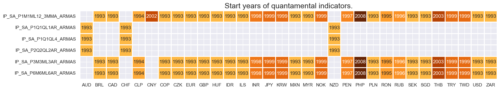
Availability #
# Availability of industry growth rates

xcatx = [xc for xc in main if xc[:3] == "IP_"]
cidx = cids
msm.check_availability(df, xcats=xcatx, cids=cidx, missing_recent=False)
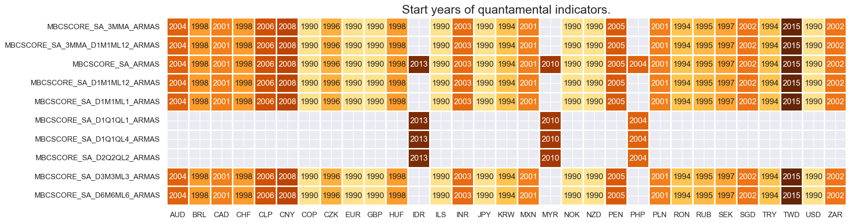
# Availability of manufacturing survey scores

xcatx = [xc for xc in main if xc[:3] == "MBC"]
cidx = cids
msm.check_availability(df, xcats=xcatx, cids=cidx, missing_recent=False)
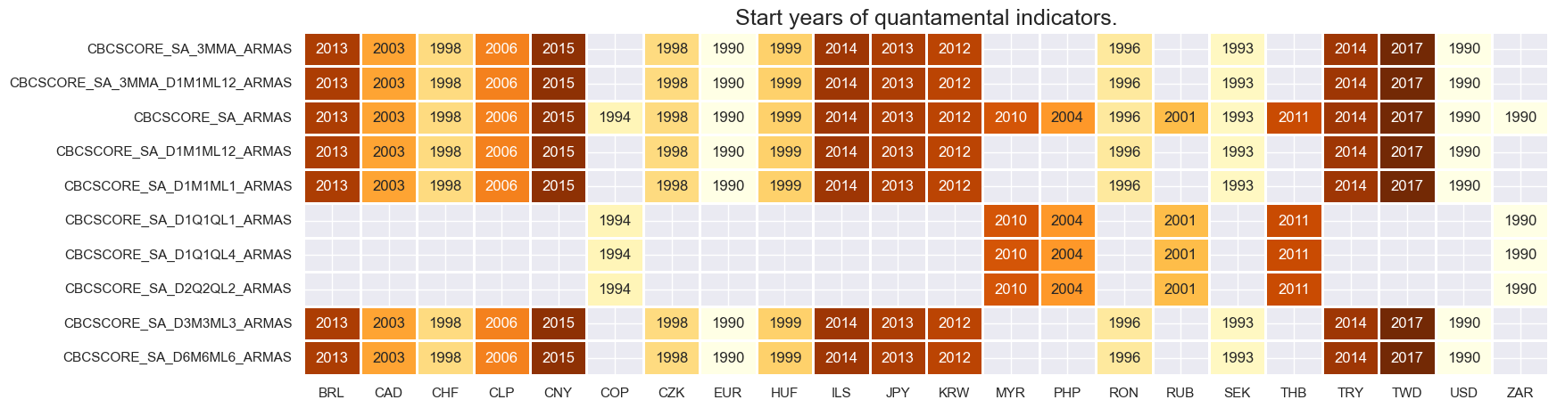
# Availability of construction survey scores

xcatx = [xc for xc in main if xc[:3] == "CBC"]
cidx = cids
msm.check_availability(dfx, xcats=xcatx, cids=cidx, missing_recent=False)
# Availability of market indicators for commodity strategy
xcatx = mark
cidx = cids_coms + ["GLD"] # Commodity cross-sections for strategy focus
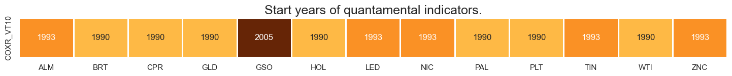
msm.check_availability(dfx, xcats=xcatx, cids=cidx, missing_recent=False)
Feature engineering and checks #
Extract base tickers and their release frequencies #
# Step 1: Extract category tickers for all base indicators of surprises
base_xcats = [xcat for xcat in main if xcat.endswith("_ARMAS")]

# Step 2: Get availability counts for each country-indicator combination
xcatx: List[str] = base_xcats
cidx: List[str] = cids
availability_counts: pd.DataFrame = (
    msm.reduce_df(dfx, xcats=xcatx, cids=cidx)
    .groupby(["cid", "xcat"], as_index=False)["value"]
    .count()
)

# Step 3: Extract observation period frequency from transformation codes
availability_counts["transformation"] = (
    availability_counts["xcat"].str.split("_").str[2]
)  # Cleaner extraction
availability_counts["frequency"] = availability_counts["transformation"].str[
    2:3
]  # 3rd character (M or Q)

# Step 4: Create country-indicator base identifiers (e.g., "AUD_IP")
availability_counts["country_indicator"] = (
    availability_counts["cid"]
    + "_"
    + availability_counts["xcat"]
    .str.split("_")
    .str[0]  # First part (IP, MBCSCORE, CBCSCORE)
)

# Step 5: Determine dominant frequency for each country-indicator combination
# (Quarterly takes precedence over monthly if both exist)
frequency_priority = {"Q": 2, "M": 1, None: 0}  # Clear priority mapping
availability_counts["freq_priority"] = availability_counts["frequency"].map(
    frequency_priority
)

# Step 6: Get the highest frequency for each country-indicator base
dominant_frequency = availability_counts.groupby("country_indicator", as_index=False)[
    "freq_priority"
].max()

# Step 7: Convert back to frequency labels and create final mapping
priority_to_freq = {2: "Q", 1: "M", 0: "M"}  # Default unknown to M
dominant_frequency["frequency"] = dominant_frequency["freq_priority"].map(
    priority_to_freq
)

# Step 8: Create final frequency dictionary
quarterly_indicators = dominant_frequency[dominant_frequency["frequency"] == "Q"][
    "country_indicator"
].tolist()
monthly_indicators = dominant_frequency[dominant_frequency["frequency"] == "M"][
    "country_indicator"
].tolist()

dict_freq = {"Q": quarterly_indicators, "M": monthly_indicators}

print(f"Quarterly indicators: {len(dict_freq['Q'])}")
print(f"Monthly indicators: {len(dict_freq['M'])}")
Quarterly indicators: 12
Monthly indicators: 73
Normalize and annualize ARMA surprises #
# Generate ARMAS surprise indicators for strategy signals
xcatx = base_xcats
cidx = cids
dfxx = msm.reduce_df(dfx, xcats=xcatx, cids=cidx)

# Create sparse dataframe with information state changes
isc_obj = msm.InformationStateChanges.from_qdf(
    df=dfxx,
    norm=True,  # normalizes changes by first release values
    std="std",
    halflife=36,  # for volatility scaling only
    min_periods=36,
    score_by="level",
)

# Convert to dense quantamental dataframe
dfa = isc_obj.to_qdf(value_column="zscore", postfix="N", thresh=3)
dfa = dfa.dropna(subset=["value"])
basic_cols = ["real_date", "cid", "xcat", "value"]
dfx = msm.update_df(dfx, dfa[basic_cols])
# Convert surprise indicators to annualized units for strategy signals
xcatx = [xc + "N" for xc in base_xcats]
cidx = cids
dfa = msm.reduce_df(dfx, xcats=xcatx, cids=cidx)
dfa["cx"] = dfa["cid"] + "_" + dfa["xcat"].str.split("_").str[0]
filt_q = dfa["cx"].isin(dict_freq["Q"])

# Apply frequency-based scaling for annualization
dfa.loc[filt_q, "value"] *= np.sqrt(1/4)    # Quarterly indicators
dfa.loc[~filt_q, "value"] *= np.sqrt(1/12)  # Monthly indicators

# Add annualized suffix and clean up
dfa["xcat"] += "A"
basic_cols = ["real_date", "cid", "xcat", "value"]
dfx = msm.update_df(dfx, dfa[basic_cols])
Rename quarterly indicators to monthly equivalents for strategy consistency #
dict_repl = {
    # Industrial production: quarterly → monthly equivalents
    "IP_SA_P1Q1QL1AR": "IP_SA_P3M3ML3AR",
    "IP_SA_P2Q2QL2AR": "IP_SA_P6M6ML6AR",
    "IP_SA_P1Q1QL4": "IP_SA_P1M1ML12_3MMA",
    # Manufacturing confidence: quarterly → monthly equivalents
    "MBCSCORE_SA_D1Q1QL1": "MBCSCORE_SA_D3M3ML3",
    "MBCSCORE_SA_D2Q2QL2": "MBCSCORE_SA_D6M6ML6",
    "MBCSCORE_SA_D1Q1QL4": "MBCSCORE_SA_3MMA_D1M1ML12",
    # Construction confidence: quarterly → monthly equivalents
    "CBCSCORE_SA_D1Q1QL1": "CBCSCORE_SA_D3M3ML3",
    "CBCSCORE_SA_D2Q2QL2": "CBCSCORE_SA_D6M6ML6",
    "CBCSCORE_SA_D1Q1QL4": "CBCSCORE_SA_3MMA_D1M1ML12",
}

# Build complete replacement mapping in one step
models = ["_ARMAS", "_ARMASN", "_ARMASNA"]
complete_replacements = {
    quarterly_indicator + suffix: monthly_indicator + suffix
    for quarterly_indicator, monthly_indicator in dict_repl.items()
    for suffix in models
}

# Transform quarterly indicators to monthly equivalents in single operation
dfx["xcat"] = dfx["xcat"].replace(complete_replacements)
dfx = dfx.sort_values(["cid", "xcat", "real_date"])
# Create user-friendly indicator names for visualization
indicator_labels = {
"IP_SA_P1M1ML12_3MMA_ARMAS": "Industry growth",
"MBCSCORE_SA_ARMAS": "Manufacturing confidence",
"CBCSCORE_SA_ARMAS": "Construction confidence",
}
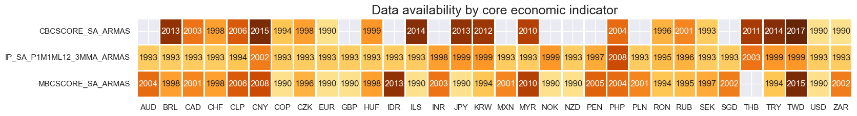
# Generate availability chart for core economic indicators
xcatx: List[str] = list(indicator_labels.keys())
cidx: List[str] = cids
msm.check_availability(
dfx,
xcats=xcatx,
cids=cidx,
missing_recent=False,
title="Data availability by core economic indicator",
start_size=(18, 2),
#xcat_labels=indicator_labels
)
# Create indicator groups for strategy signal construction
def filter_by_indicator_type(indicators: List[str]) -> Dict[str, List[str]]:
    """Group indicators by economic report type."""
    return {
        'industrial': [ind for ind in indicators if ind.startswith("IP_")],
        'manufacturing': [ind for ind in indicators if ind.startswith("MBC")],
        'construction': [ind for ind in indicators if ind.startswith("CBC")]
    }

# Annualized surprise indicators (available in dataset)
available_armas: List[str] = list(set(base_xcats) & set(dfx.xcat.unique()))  # Remove quarterly (non-existing)
annualized_surprises: List[str] = [xc + "NA" for xc in available_armas]
surprise_groups: Dict[str, List[str]] = filter_by_indicator_type(annualized_surprises)

print(f"Surprise indicators: {len(annualized_surprises)}")
Surprise indicators: 17
Composite economic surprises (across transformations of base indicator) #
# Create linear composites of surprises and changes
cidx = cids

# Surprises configuration
dict_surprises: Dict[str, List[str]] = {
    "IND": surprise_groups["industrial"],
    "MBC": surprise_groups["manufacturing"],
    "CBC": surprise_groups["construction"],
}
composite_dfs = []

# Create surprise composites
for base, xcatx in dict_surprises.items():
    with warnings.catch_warnings():
        warnings.simplefilter("ignore", category=UserWarning)
        composite_dfs.append(msp.linear_composite(dfx, xcats=xcatx, cids=cidx, new_xcat=f"{base}_ARMASNA"))

# Store in main dataframe
dfa = pd.concat(composite_dfs, axis=0, ignore_index=True)
dfx = msm.update_df(dfx, dfa)

# Labels and list of composite factors
dict_csnames: Dict[str, List[str]] = {
    "IND_ARMASNA": "Industrial production composite",
    "MBC_ARMASNA": "Manufacturing business confidence composite",
    "CBC_ARMASNA": "Construction business confidence composite",
}
comp_surprises = [key for key in dict_csnames.keys()]
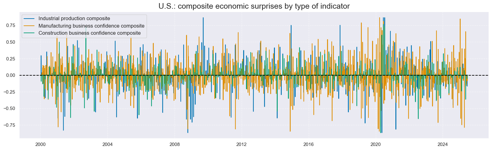
# Inspect time-series of linear composite factors

xcatx = comp_surprises
cidx = ["USD"]
msp.view_timelines(
    dfx,
    xcats=xcatx,
    cids=cidx,
    ncol=3,
    title="U.S.: composite economic surprises by type of indicator",
    size=(16, 5),
    xcat_labels=dict_csnames,
    start="2000-01-01",
)
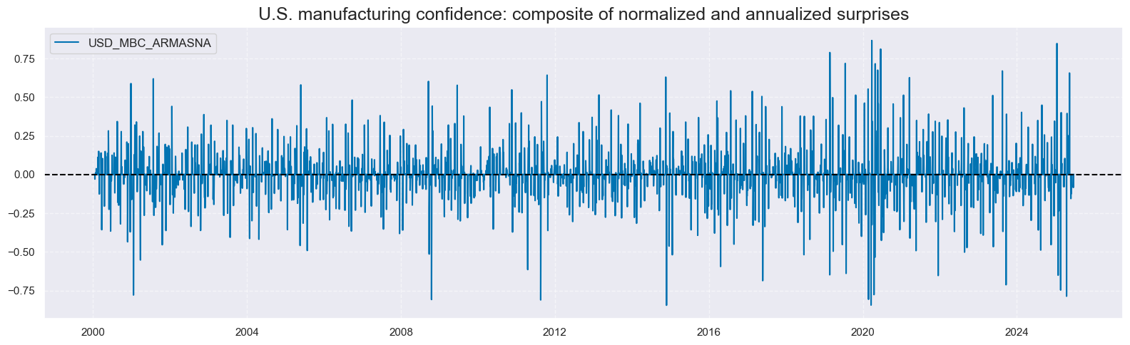
# Inspect time-series of specific linear composite factor

xcatx = ["MBC_ARMASNA"]
cidx = ["USD"]
msp.view_timelines(
    dfx,
    xcats=xcatx,
    cids=cidx,
    title="U.S. manufacturing confidence: composite of normalized and annualized surprises",
    size=(16, 5),
    start="2000-01-01",
)
Exponentially moving sums #
xcatx = comp_surprises
cidx = cids
hts = [3] # Half-lives
dfa = msm.reduce_df(dfx, xcats=xcatx, cids=cidx)
dfa["ticker"] = dfa["cid"] + "_" + dfa["xcat"]
p = dfa.pivot(index="real_date", columns="ticker", values="value")
store = []
for ht in hts:
proll = p.ewm(halflife=ht).sum()
proll.columns += f"_{ht}DXMS"
df_temp = proll.stack().to_frame("value").reset_index()
df_temp[["cid", "xcat"]] = df_temp["ticker"].str.split("_", n=1, expand=True)
store.append(df_temp[["cid", "xcat", "real_date", "value"]])
dfx = msm.update_df(dfx, pd.concat(store, axis=0, ignore_index=True))
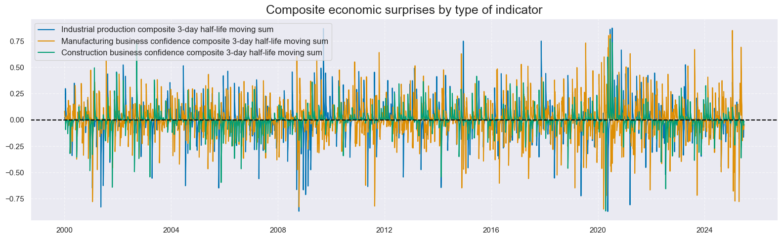
# Generate lists of moving sum indicators
dict_csnames_3d = {
k + "_3DXMS": v + " 3-day half-life moving sum" for k, v in dict_csnames.items()
}
comp_surprises_3d = [key for key in dict_csnames_3d.keys()]
# Inspect time-series of linear composite factors

xcatx = comp_surprises_3d
cidx = ["USD"]
msp.view_timelines(
    dfx,
    xcats=xcatx,
    cids=cidx,
    ncol=3,
    title="Composite economic surprises by type of indicator",
    size=(16, 5),
    xcat_labels=dict_csnames_3d,
    start="2000-01-01",
)
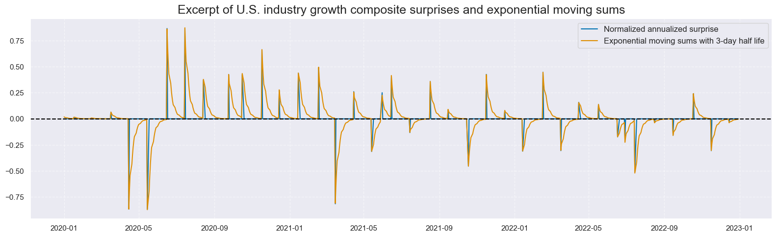
xc = "IND"
xcatx = [xc + "_ARMASNA", xc + "_ARMASNA_3DXMS"]
cidx = ["USD"]

msp.view_timelines(
    dfx,
    xcats=xcatx,
    cids=cidx,
    start="2020-01-01",
    end="2023-01-01",
    title="Excerpt of U.S. industry growth composite surprises and exponential moving sums",
    xcat_labels=[
        "Normalized annualized surprise",
        "Exponential moving sums with 3-day half life",
    ],
    size=(16, 5),
)
Global composite surprises #
# Create global weighted composites using investment value-added weights
xcatx: List[str] = comp_surprises_3d
cidx: List[str] = cids
store: List[pd.DataFrame] = []

for xcat in xcatx:
    dfr = msm.reduce_df(dfx, cids=cidx, xcats=[xcat, "IVAWGT_SA_1YMA"])
    with warnings.catch_warnings():
        warnings.simplefilter("ignore", category=UserWarning)
        dfa = msp.linear_composite(
            df=dfr,
            xcats=xcat,
            cids=cidx,
            weights="IVAWGT_SA_1YMA",
            new_cid="GLB",
            complete_cids=False,
        )
    store.append(dfa)

dfx = msm.update_df(dfx, pd.concat(store, axis=0, ignore_index=True))
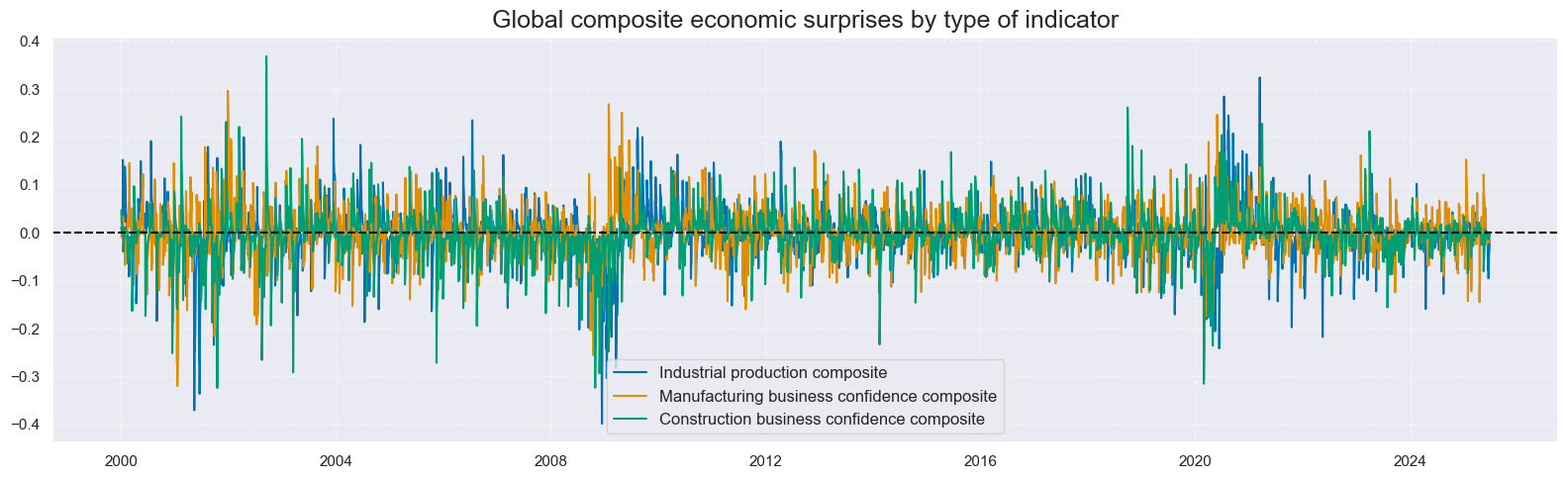
# Plot global composite signals by indicator type
cidx: List[str] = ["GLB"]
xcatx: List[str] = comp_surprises_3d

# Restructure data for plotting multiple series on single charts
dfa = msm.reduce_df(dfx, xcats=xcatx, cids=cidx)
dfa["ticker"] = dfa["cid"] + "_" + dfa["xcat"]
dfa["cid"] = dfa["ticker"].str[4:7]     # Extract indicator type (IND, MBC, CBC)
dfa["xcat"] = dfa["ticker"].str[8:]     # Extract signal type for comparison

# Labels and list of composite factors
dict_csnames_3d: Dict[str, List[str]] = {
    "IND_ARMASNA_3DXMS": "Industrial production composite",
    "MBC_ARMASNA_3DXMS": "Manufacturing business confidence composite",
    "CBC_ARMASNA_3DXMS": "Construction business confidence composite",
}

msp.view_timelines(
    dfx,
    xcats=xcatx,
    cids=cidx,
    ncol=3,
    title="Global composite economic surprises by type of indicator",
    size=(16, 5),
    xcat_labels=dict_csnames_3d,
    start="2000-01-01",
)
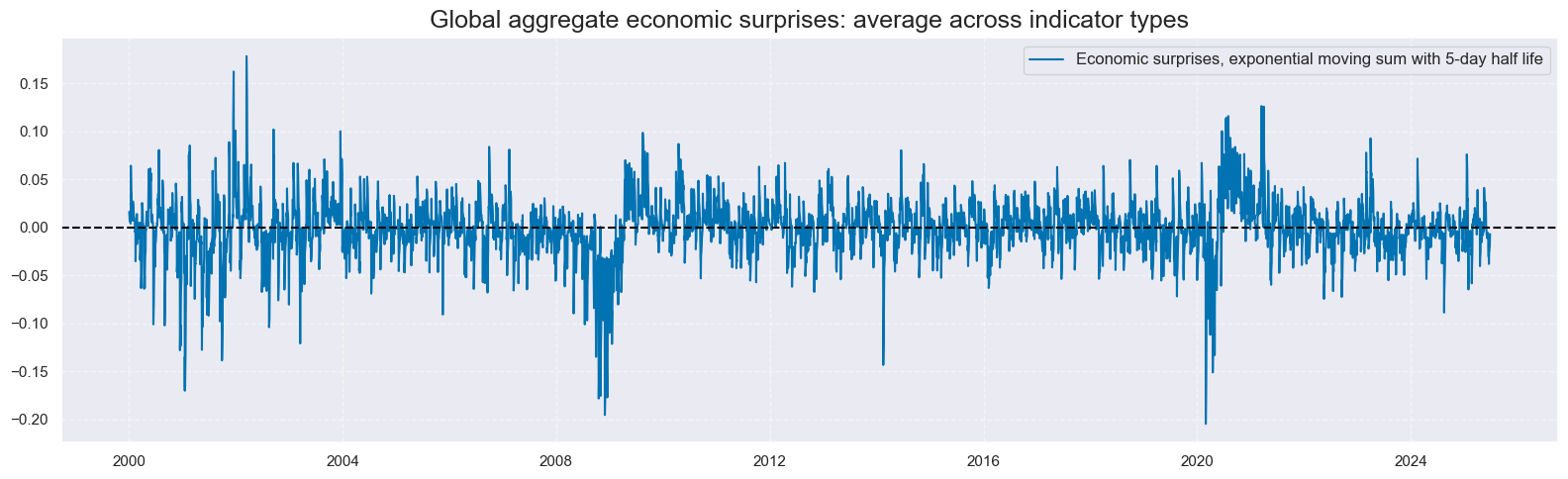
Grand total global economic surprises #
# Create global aggregates across indicator categories (IND + MBC + CBC)
cidx: List[str] = ["GLB"]
dict_aggs: Dict[str, List[str]] = {
"ARMASNA_3DXMS": comp_surprises_3d, # 3-day surprise aggregate
}
store: List[pd.DataFrame] = []
for aggregate_name, component_xcats in dict_aggs.items():
store.append(msp.linear_composite(dfx, xcats=component_xcats, cids=cidx, new_xcat=aggregate_name))
dfx = msm.update_df(dfx, pd.concat(store, axis=0, ignore_index=True))
# Store list of global aggregate indicators
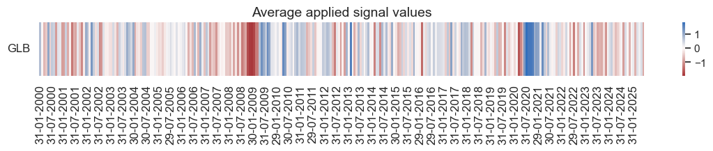
global_aggregates: List[str] = list(dict_aggs.keys())
xcat_labels = {
    "ARMASNA_3DXMS": "Economic surprises, exponential moving sum with 5-day half life"
}
xcatx = list(xcat_labels.keys())
cidx = ["GLB"]

msp.view_timelines(
    dfx,
    xcats=xcatx,
    cids=cidx,
    title="Global aggregate economic surprises: average across indicator types",
    xcat_labels=xcat_labels,
    size=(16, 5),
    start="2000-01-01",
)
Target returns and checks #
Vol-targeted contract returns #
# Industrial commodities
cidx = cids_coms
xcatx = ["COXR_VT10"]

dict_coms: Dict[str, List[str]] = {
    "BRT": "Brent crude oil",
    "WTI": "West Texas Intermediate crude oil",
    "GSO": "Gasoline",
    "HOL": "Heating oil",
    "ALM": "Aluminum",
    "CPR": "Copper",
    "LED": "Lead",
    "NIC": "Nickel",
    "TIN": "Tin",
    "ZNC": "Zinc",
    "PAL": "Palladium",
    "PLT": "Platinum",
    "NGS": "Natural gas",
}

msp.view_timelines(
    dfx,
    xcats=xcatx,
    cids=cidx,
    cumsum=True,
    title="Industrial commodities: cumulative vol-targeted futures returns since 2000",
    title_fontsize=24,
    cid_labels=dict_coms,
    same_y=True,
    size=(14, 6),
    aspect=1.75,
    single_chart=False,
    start="2000-01-01",
)
cidx = cids_coms
xcatx = ["COXR_VT10"]

msv.view_correlation(
    df=dfx,
    xcats=xcatx,
    cids=cidx,
    cluster=True,
    freq="M",
    title="Futures returns correlation across industrial commodities, monthly averages, since 2000",
    title_fontsize=18,
    size=(16, 8),
    start="2000-01-01",
)
Hedged vol-targeted contract returns #
store: List[str] = []
cidx = cids_coms

with warnings.catch_warnings():
    warnings.simplefilter("ignore", category=UserWarning)
    dfh = msp.return_beta(
        dfx,
        xcat="COXR_VT10",
        cids=cidx,
        benchmark_return="GLD_COXR_VT10",
        oos=True,
        min_obs=24,
        max_obs=60,
        hedged_returns=True,
        # start="2000-01-01",
        refreq="m",
        hr_name="HvGLD",
    )
    dfh.xcat = dfh.xcat.cat.rename_categories({"COXR_VT10_HR": "COXR_BETAvGLD"})

dfx = msm.update_df(df=dfx, df_add=dfh, xcat_replace=True)
# Plot the betas
xcatx: List[str] = ["COXR_BETAvGLD"]
cidx = cids_coms

msv.timelines(
    dfx,
    xcats=xcatx,
    cids=cidx,
    start="2000-01-01",
    ncol=6,
    title="Industrial commodity future betas to gold futures returns",
    title_fontsize=20,
    cid_labels=dict_coms,
    height=2,
    aspect=1,
    single_chart=False,
    ax_hline=0,
)
# Plot hedged returns
xcatx: List[str] = ["COXR_VT10", "COXR_VT10_HvGLD",]
cidx = cids_coms

msp.view_timelines(
    dfx,
    xcats=xcatx,
    cids=cidx,
    # start="2000-01-01",
    cumsum=True,
    title="Industrial commodities: cumulative vol-targeted futures returns",
    title_fontsize=24,
    cid_labels=dict_coms,
    xcat_labels=["unhedged returns", "hedged returns"],
    same_y=True,
    size=(14, 6),
    aspect=1.75,
    single_chart=False,
    start="2000-01-01",
)
Commodity basket returns #
# Create basket against Gold
store = []
baskets: List[Tuple[str, List[str]]] = [("", cids_coms), ("BAMS", cids_bams), ("PRMS", cids_prms), ("FUEN", cids_fuen)]
targets = ["", "_HvGLD"]
for cat, cidx in baskets:
    for target in targets:
        xcat = f"COXR_VT10{target}"

        dfa = msp.linear_composite(
            df=msm.reduce_df(dfx, xcats=[xcat], cids=cidx),
            xcats=xcat,
            cids=cidx,
            weights=None,  # equal weights
            new_cid="GLB",
            complete_cids=False,  # uses available contracts only
        )

        # Rename to basket of commodities
        dfa["xcat"] = f"CO{cat:s}XR_VT10{target:s}"
        store.append(dfa)

dfx = msm.update_df(dfx, pd.concat(store, axis=0, ignore_index=True))
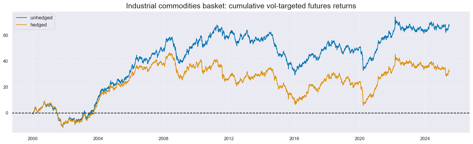
# Plot basket returns
targets = ["", "_HvGLD"]
xcatx: List[str] = [f"COXR_VT10{target:s}" for target in targets]
cidx = ["GLB"]

msp.view_timelines(
    dfx,
    xcats=xcatx,
    cids=cidx,
    cumsum=True,
    title="Industrial commodities basket: cumulative vol-targeted futures returns",

    xcat_labels=[
        "unhedged",
        "hedged",
    ],
    size=(16, 5),
    start="2000-01-01",
)
Value checks #
Unhedged basket trading #
Specs and panel test #
dict_unhedged = {
    "sig": "ARMASNA_3DXMS",
    "targ": "COXR_VT10",
    "cidx": ["GLB"],
    "start": "2000-01-01",
    "black": None,
    "crr": None,
    "srr": None,
    "pnls": None,
}
dix = dict_unhedged
sig = dix["sig"]
targ = dix["targ"]
cidx = dix["cidx"]
start = dix["start"]
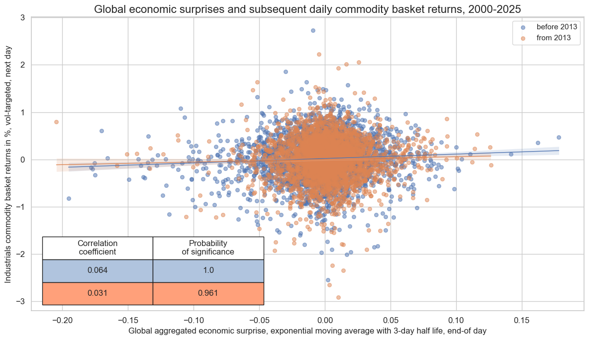
crx = msp.CategoryRelations(
dfx,
xcats=[sig, targ],
cids=cidx,
freq="D",
lag=1,
xcat_aggs=["last", "sum"],
start=start,
)
with warnings.catch_warnings():
warnings.simplefilter("ignore")
crx.reg_scatter(
labels=False,
coef_box="lower left",
separator=2013,
title="Global economic surprises and subsequent daily commodity basket returns, 2000-2025",
title_fontsize=16,
xlab="Global aggregated economic surprise, exponential moving average with 3-day half life, end-of day",
ylab="Industrials commodity basket returns in %, vol-targeted, next day",
size=(12, 7),
prob_est="map",
)
Accuracy and correlation check #
dix = dict_unhedged

sig = dix["sig"]
targ = dix["targ"]
cidx = dix["cidx"]
start = dix["start"]

srr = mss.SignalReturnRelations(
    dfx,
    cids=cidx,
    sigs=sig,
    rets=targ,
    freqs="D",
    start=start,
)

dix["srr"] = srr
dix = dict_unhedged
srr = dix["srr"]
display(srr.multiple_relations_table().astype("float").round(3).T)
| Return | COXR_VT10 |
|---|---|
| Signal | ARMASNA_3DXMS |
| Frequency | D |
| Aggregation | last |
| accuracy | 0.517 |
| bal_accuracy | 0.517 |
| pos_sigr | 0.501 |
| pos_retr | 0.527 |
| pos_prec | 0.545 |
| neg_prec | 0.490 |
| pearson | 0.048 |
| pearson_pval | 0.000 |
| kendall | 0.025 |
| kendall_pval | 0.002 |
| auc | 0.517 |
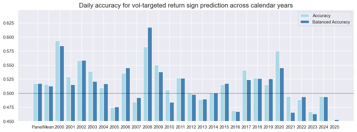
dix = dict_unhedged
srr = dix["srr"]

srr.accuracy_bars(
    type="years",
    title="Daily accuracy for vol-targeted return sign prediction across calendar years",
    size=(15, 5),
)
Naive PnL #
dix = dict_unhedged
sig = dix["sig"]
targ = dix["targ"]
cidx = dix["cidx"]
start = dix["start"]
naive_pnl = msn.NaivePnL(
dfx,
ret=targ,
sigs=[sig],
cids=cidx,
start=start,
bms=["USD_EQXR_NSA"],
)
for long_bias in (0, 1):
naive_pnl.make_pnl(
sig,
sig_neg=False,
sig_op="zn_score_cs",
sig_add=long_bias,
thresh=2,
rebal_freq="daily",
vol_scale=None,
rebal_slip=0,
pnl_name=sig + f"_PZN{long_bias:d}",
)
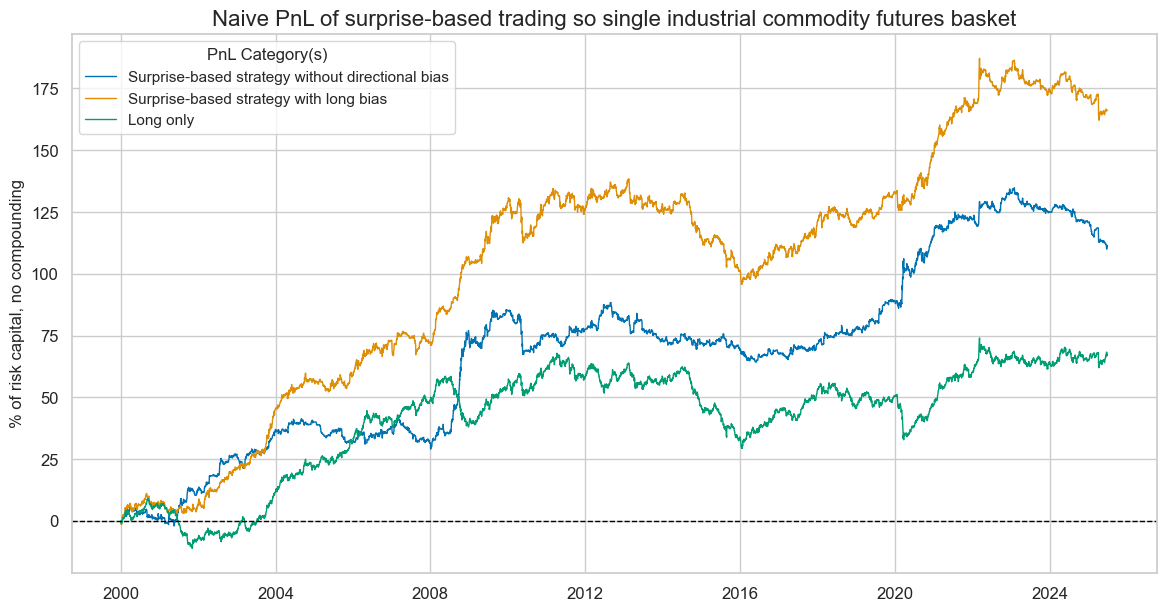
naive_pnl.make_long_pnl(vol_scale=None, label="Long only")
dix["pnls"] = naive_pnl
dix = dict_unhedged
naive_pnl = dix["pnls"]
sig = dix["sig"]
pnl_labels = {
    f"{sig:s}_PZN0": "Surprise-based strategy without directional bias",
    f"{sig:s}_PZN1": "Surprise-based strategy with long bias",
    "Long only": "Long only",
}
pnls = list(pnl_labels.keys())

naive_pnl.plot_pnls(
    pnl_cats=pnls,
    pnl_cids=["ALL"],
    start=start,
    title="Naive PnL of surprise-based trading so single industrial commodity futures basket",
    title_fontsize=16,
    xcat_labels=pnl_labels,
    figsize=(14, 7),
)
dix = dict_unhedged
naive_pnl = dix["pnls"]

display(naive_pnl.evaluate_pnls())

naive_pnl.signal_heatmap(
    pnl_name="ARMASNA_3DXMS_PZN1",
    freq="m",
)
| xcat | ARMASNA_3DXMS_PZN0 | ARMASNA_3DXMS_PZN1 | Long only |
|---|---|---|---|
| Return % | 4.37104 | 6.523791 | 2.635708 |
| St. Dev. % | 7.427 | 8.913999 | 7.191436 |
| Sharpe Ratio | 0.588534 | 0.731859 | 0.366506 |
| Sortino Ratio | 0.882928 | 1.035662 | 0.507064 |
| Max 21-Day Draw % | -15.375868 | -17.217568 | -14.302399 |
| Max 6-Month Draw % | -16.807392 | -20.328708 | -20.143069 |
| Peak to Trough Draw % | -24.853876 | -42.617399 | -38.519882 |
| Top 5% Monthly PnL Share | 0.938577 | 0.610671 | 1.030927 |
| USD_EQXR_NSA correl | -0.075653 | 0.145845 | 0.286987 |
| Traded Months | 306 | 306 | 306 |
Hedged basket trading #
Specs and panel test #
dict_hedged = {
    "sig": "ARMASNA_3DXMS",
    "targ": "COXR_VT10_HvGLD",
    "cidx": ["GLB"],
    "start": "2000-01-01",
    "black": None,
    "crr": None,
    "srr": None,
    "pnls": None,
}
dix = dict_hedged
sig = dix["sig"]
targ = dix["targ"]
cidx = dix["cidx"]
start = dix["start"]
crx = msp.CategoryRelations(
dfx,
xcats=[sig, targ],
cids=cidx,
freq="D",
lag=1,
xcat_aggs=["last", "sum"],
start=start,
)
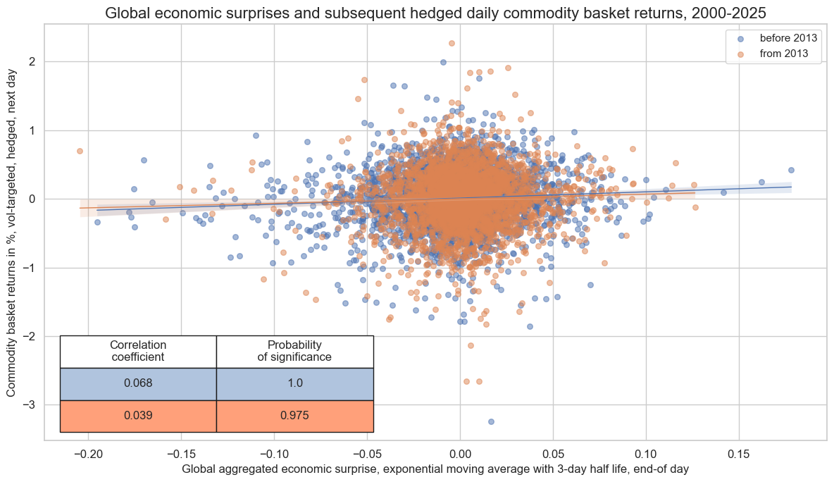
with warnings.catch_warnings():
warnings.simplefilter("ignore")
crx.reg_scatter(
labels=False,
coef_box="lower left",
separator=2013,
xlab="Global aggregated economic surprise, exponential moving average with 3-day half life, end-of day",
ylab="Commodity basket returns in %, vol-targeted, hedged, next day",
title="Global economic surprises and subsequent hedged daily commodity basket returns, 2000-2025",
title_fontsize=16,
size=(12, 7),
prob_est="map",
)
Accuracy and correlation check #
dix = dict_hedged

sig = dix["sig"]
targ = dix["targ"]
cidx = dix["cidx"]
start = dix["start"]

srr = mss.SignalReturnRelations(
    dfx,
    cids=cidx,
    sigs=sig,
    rets=targ,
    freqs="D",
    start=start,
)

dix["srr"] = srr
dix = dict_hedged
srr = dix["srr"]
display(srr.multiple_relations_table().astype("float").round(3).T)
| Return | COXR_VT10_HvGLD |
|---|---|
| Signal | ARMASNA_3DXMS |
| Frequency | D |
| Aggregation | last |
| accuracy | 0.508 |
| bal_accuracy | 0.508 |
| pos_sigr | 0.501 |
| pos_retr | 0.525 |
| pos_prec | 0.533 |
| neg_prec | 0.483 |
| pearson | 0.054 |
| pearson_pval | 0.000 |
| kendall | 0.026 |
| kendall_pval | 0.002 |
| auc | 0.508 |
Naive PnL #
dix = dict_hedged

sig = dix["sig"]
targ = dix["targ"]
cidx = dix["cidx"]
start = dix["start"]

naive_pnl = msn.NaivePnL(
    dfx,
    ret=targ,
    sigs=[sig],
    cids=cidx,
    start=start,
    bms=["USD_EQXR_NSA"],
)

for long_bias in (0, 1):
    naive_pnl.make_pnl(
        sig,
        sig_neg=False,
        sig_op="zn_score_cs",
        sig_add=long_bias,
        thresh=2,
        rebal_freq="daily",
        vol_scale=None,
        rebal_slip=0,
        pnl_name=sig + f"_PZN{long_bias:d}",
    )

naive_pnl.make_long_pnl(vol_scale=None, label="Long only")

dix["pnls"] = naive_pnl
dix = dict_hedged
naive_pnl = dix["pnls"]
sig = dix["sig"]
pnl_labels = {
    f"{sig:s}_PZN0": "Surprise-based strategy without directional bias",
    f"{sig:s}_PZN1": "Surprise-based strategy with long bias",
    "Long only": "Long only",
}
pnls = list(pnl_labels.keys())

naive_pnl.plot_pnls(
    pnl_cats=pnls,
    pnl_cids=["ALL"],
    start=start,
    title="Naive PnL of surprise-based trading of single hedged industrial commodity futures basket",
    title_fontsize=16,
    xcat_labels=pnl_labels,
    figsize=(14, 7),
)
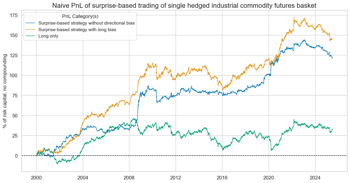
dix = dict_hedged
naive_pnl = dix["pnls"]
display(naive_pnl.evaluate_pnls())
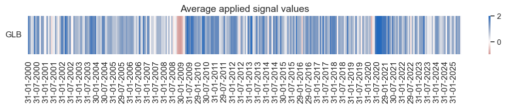
naive_pnl.signal_heatmap(
pnl_name="ARMASNA_3DXMS_PZN0",
freq="m",
)
| xcat | ARMASNA_3DXMS_PZN0 | ARMASNA_3DXMS_PZN1 | Long only |
|---|---|---|---|
| Return % | 4.792582 | 5.706744 | 1.268342 |
| St. Dev. % | 7.02999 | 8.322689 | 6.660833 |
| Sharpe Ratio | 0.681734 | 0.685685 | 0.190418 |
| Sortino Ratio | 1.046182 | 0.967819 | 0.26069 |
| Max 21-Day Draw % | -15.713679 | -19.359406 | -13.492343 |
| Max 6-Month Draw % | -17.007099 | -19.048991 | -19.006064 |
| Peak to Trough Draw % | -23.609668 | -33.977972 | -40.533251 |
| Top 5% Monthly PnL Share | 0.846206 | 0.683088 | 2.084462 |
| USD_EQXR_NSA correl | -0.084836 | 0.152752 | 0.307985 |
| Traded Months | 306 | 306 | 306 |