Macro trends and sectoral equity performance

This notebook offers the necessary code to replicate the research findings discussed in the Macrosynergy research post “Macro trends and sectoral equity performance”. Its primary objective is to inspire readers to explore and conduct additional investigations whilst also providing a foundation for testing their own unique ideas.

Macroeconomic trends, such as economic growth, affect stocks differently, depending on their lines of business and their home markets. This means that point-in-time macro trend indicators can support two types of investment decisions: allocation across sectors within the same country and allocation across countries within the same sector. Panel analysis for 11 sectors and 12 countries over the last 25 years reveals examples for both. Across sectors, export growth, services business sentiment, and consumer confidence have predicted the outperformance of energy stocks, services stocks, and real estate stocks respectively. Across countries, relative export growth, manufacturing sentiment changes, and financial conditions have predicted the outperformance of local stocks versus foreign ones, for the overall market and within sectors.

The notebook covers the three main parts:

• Get Packages and JPMaQS Data: This section is responsible for installing and importing the necessary Python packages used throughout the analysis.

• Transformations and checks: In this part, the notebook performs calculations and transformations on the data to derive the relevant signals and targets used for the analysis, including building simple linear composite indicators.

• Value checks: This is the most critical section, where the notebook calculates and implements the trading strategies based on the hypotheses tested in the post. This section involves backtesting simple trading strategies.

It is important to note that while the notebook covers a selection of indicators and strategies used for the post’s main findings, users can explore countless other possible indicators and approaches. Users can modify the code to test different hypotheses and strategies based on their research and ideas. Best of luck with your research!

Get packages and JPMaQS data

This notebook primarily relies on the standard packages available in the Python data science stack. However, there is an additional package macrosynergy that is required for two purposes:

• Downloading JPMaQS data: The macrosynergy package facilitates the retrieval of JPMaQS data, which is used in the notebook.

• For the analysis of quantamental data and value propositions: The macrosynergy package provides functionality for performing quick analyses of quantamental data and exploring value propositions.

For detailed information and a comprehensive understanding of the macrosynergy package and its functionalities, please refer to the “Introduction to Macrosynergy package” notebook on the Macrosynergy Quantamental Academy or visit the following link on Kaggle .

# Run only if needed!
# !pip install macrosynergy --upgrade

import numpy as np
import pandas as pd
from pandas import Timestamp
import matplotlib.pyplot as plt
import seaborn as sns

import copy
import warnings
import os

import macrosynergy.management as msm
import macrosynergy.panel as msp
import macrosynergy.signal as mss
import macrosynergy.pnl as msn
import macrosynergy.visuals as msv
from macrosynergy.download import JPMaQSDownload

warnings.simplefilter("ignore")

This notebook downloads selected indicators for the following cross-sections: AUD (Australian dollar), CAD (Canadian dollar), CHF (Swiss franc), EUR (euro), GBP (British pound), HKD (Hong Kong dollar), ILS (Israeli shekel), JPY (Japanese yen), NOK (Norwegian krone), NZD (New Zealand dollar), SEK (Swedish krona), SGD (Singapore dollar), USD (U.S. dollar) as well as five main European currencies [‘DEM’, ‘ESP’, ‘FRF’, ‘ITL’, ‘NLG’], replaced by EUR.

# Equity cross-section lists

# Cross-sections of interest
cids_dmeq = ['AUD', 'CAD', 'CHF', 'EUR', 'GBP', 'HKD', 'ILS', 'JPY', 'NOK', 'NZD', 'SEK', 'SGD', 'USD']
cids_eueq = ['DEM', 'ESP', 'FRF', 'ITL', 'NLG']

cids = sorted(cids_dmeq + cids_eueq)
cids_eqx = list(set(cids_dmeq) - {'HKD'})

sector_labels = {
    "ALL": "All sectors", 
    "COD": "Cons. discretionary",
    "COS": "Cons. staples",
    "CSR": "Communication services",
    "ENR": "Energy",
    "FIN": "Financials",
    "HLC": "Healthcare",
    "IND": "Industrials",
    "ITE": "Information tech",
    "MAT": "Materials",
    "REL": "Real estate",
    "UTL": "Utilities",
}
secx = list(sector_labels.keys())
secs = list(sector_labels.keys())[1:]

JPMaQS indicators are conveniently grouped into 6 main categories: Economic Trends, Macroeconomic balance sheets, Financial conditions, Shocks and risk measures, Stylized trading factors, and Generic returns. Each indicator has a separate page with notes, description, availability, statistical measures, and timelines for main currencies. The description of each JPMaQS category is available either under JPMorgan Markets (password protected) or the Macro Quantamental Academy . In particular, the indicators used in this notebook can be found under Manufacturing confidence scores , Industrial production trends , Foreign trade trends , Services confidence scores , Private consumption , Global production shares , Private credit expansion , Consumer price inflation trends , U.S. special data , GDP growth , Intuitive GDP growth estimates , Inflation targets , and Real interest rates ,

# Category tickers

# Economic indicators

manuf = [
    # Manufacturing confidence scores
    "MBCSCORE_SA",
    "MBCSCORE_SA_D3M3ML3",
    "MBCSCORE_SA_D1Q1QL1",
    # Short term industrial production trend
    "IP_SA_P3M3ML3AR",
    "IP_SA_P6M6ML6AR",
    "IP_SA_P1M1ML12_3MMA",
    # Export growth
    "EXPORTS_SA_P6M6ML6AR",
    "EXPORTS_SA_P1M1ML12_3MMA"
]
servi = [
    # Service confidence scores
    "SBCSCORE_SA",
    "SBCSCORE_SA_D3M3ML3",
    "SBCSCORE_SA_D1Q1QL1",
]
consu = [
    # Consumer confidence scores
    "CCSCORE_SA",
    "CCSCORE_SA_D3M3ML3",
    "CCSCORE_SA_D1Q1QL1",
    # private credit
    "PCREDITBN_SJA_P1M1ML12", 
]
cpi = [
    # Consumer core inflation: YoY, QoQ annualised
    "CPIC_SA_P1M1ML12",
    "CPIC_SJA_P3M3ML3AR",
]
ppi = [
    # Producer Inflation: YoY, QoQ annualised
    "PPIH_NSA_P1M1ML12",
    "PPIH_SA_P3M3ML3AR",
]

ecos = manuf + servi + consu + cpi + ppi

# Complementary economic indicators
ecox = [
    "IVAWGT_SA_1YMA",
    "USDGDPWGT_SA_1YMA",
    "RGDP_SA_P1Q1QL4_20QMM",
    "INTRGDP_NSA_P1M1ML12_3MMA",
    "INFTEFF_NSA",
    "RYLDIRS02Y_NSA",
    "RYLDIRS05Y_NSA",
]

# Market indicators
eqrets = ["EQC" + sec + ret for sec in secx for ret in ["R_NSA", "XR_NSA"]]
eqblack = ["EQC" + sec + "UNTRADABLE_NSA" for sec in secx]
fxrets = ["FXXRUSD_NSA"]
marks = eqrets + eqblack + fxrets

# All indicators
xcats = ecos + ecox + marks

# Resultant tickers
tickers = [cid + "_" + xcat for cid in cids for xcat in xcats]
print(f"Maximum number of tickers is {len(tickers)}")

Maximum number of tickers is 1134

The JPMaQS indicators we consider are downloaded using the J.P. Morgan Dataquery API interface within the macrosynergy package. This is done by specifying ticker strings, formed by appending an indicator category code to a currency area code <cross_section>. These constitute the main part of a full quantamental indicator ticker, taking the form DB(JPMAQS,<cross_section>_<category>,<info>) , where denotes the time series of information for the given cross-section and category. The following types of information are available:

value giving the latest available values for the indicator eop_lag referring to days elapsed since the end of the observation period mop_lag referring to the number of days elapsed since the mean observation period grade denoting a grade of the observation, giving a metric of real-time information quality.

After instantiating the JPMaQSDownload class within the macrosynergy.download module, one can use the download(tickers,start_date,metrics) method to easily download the necessary data, where tickers is an array of ticker strings, start_date is the first collection date to be considered and metrics is an array comprising the times series information to be downloaded. For more information see here .

client_id: str = os.getenv("DQ_CLIENT_ID")
client_secret: str = os.getenv("DQ_CLIENT_SECRET")

with JPMaQSDownload(oauth=True, client_id=client_id, client_secret=client_secret) as dq:
    assert dq.check_connection()
    df = dq.download(
        tickers=tickers,
        start_date="1990-01-01",
        suppress_warning=True,
        metrics=["value"],
        show_progress=True,
    )
    assert isinstance(df, pd.DataFrame) and not df.empty

#print("Last updated:", date.today())

Downloading data from JPMaQS.
Timestamp UTC:  2025-03-05 15:53:05
Connection successful!

Requesting data: 100%|██████████| 57/57 [00:11<00:00,  4.97it/s]
Downloading data: 100%|██████████| 57/57 [00:40<00:00,  1.41it/s]

Some expressions are missing from the downloaded data. Check logger output for complete list.
125 out of 1134 expressions are missing. To download the catalogue of all available expressions and filter the unavailable expressions, set `get_catalogue=True` in the call to `JPMaQSDownload.download()`.
Some dates are missing from the downloaded data. 
2 out of 9180 dates are missing.

dfx = df.copy().sort_values(["cid", "xcat", "real_date"])
dfx.info()

<class 'pandas.core.frame.DataFrame'>
Index: 8375198 entries, 36273 to 8368261
Data columns (total 4 columns):
 #   Column     Dtype         
---  ------     -----         
 0   real_date  datetime64[ns]
 1   cid        object        
 2   xcat       object        
 3   value      float64       
dtypes: datetime64[ns](1), float64(1), object(2)
memory usage: 319.5+ MB

Renaming and availability

Rename quarterly tickers to roughly equivalent monthly tickers to simplify subsequent operations.

dict_repl = {
    # surveys
    "CCSCORE_SA_D1Q1QL1": "CCSCORE_SA_D3M3ML3",
    "SBCSCORE_SA_D1Q1QL1": "SBCSCORE_SA_D3M3ML3",
    "MBCSCORE_SA_D1Q1QL1": "MBCSCORE_SA_D3M3ML3",
}

for key, value in dict_repl.items():
    dfx["xcat"] = dfx["xcat"].str.replace(key, value)

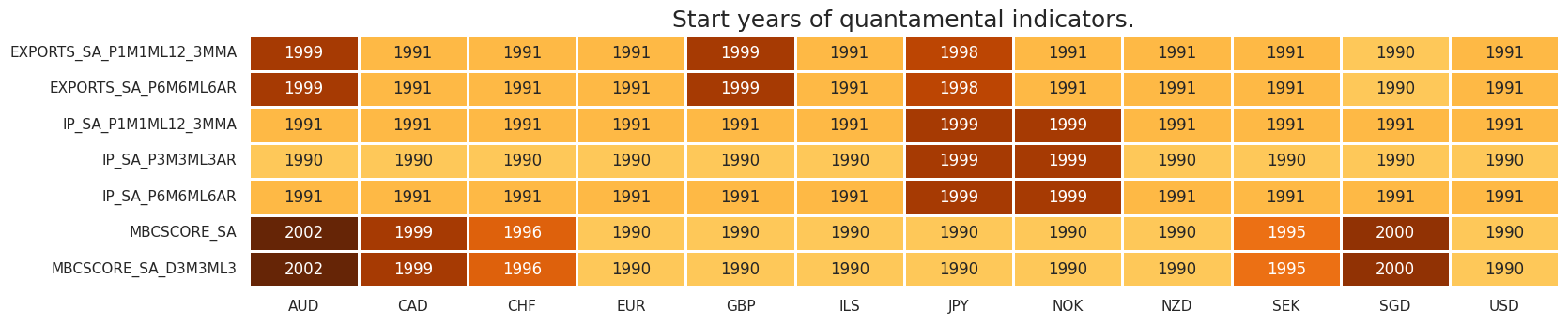
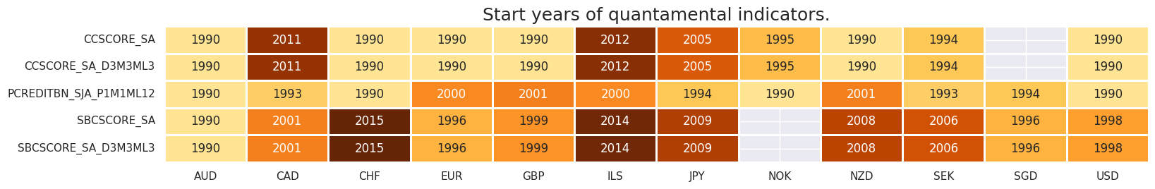
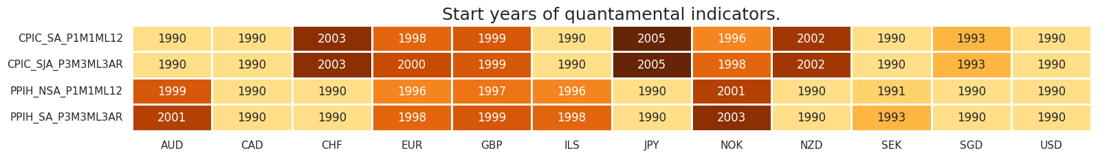
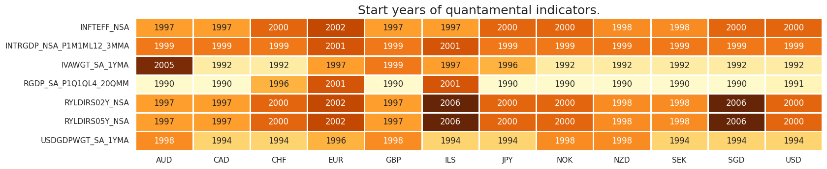
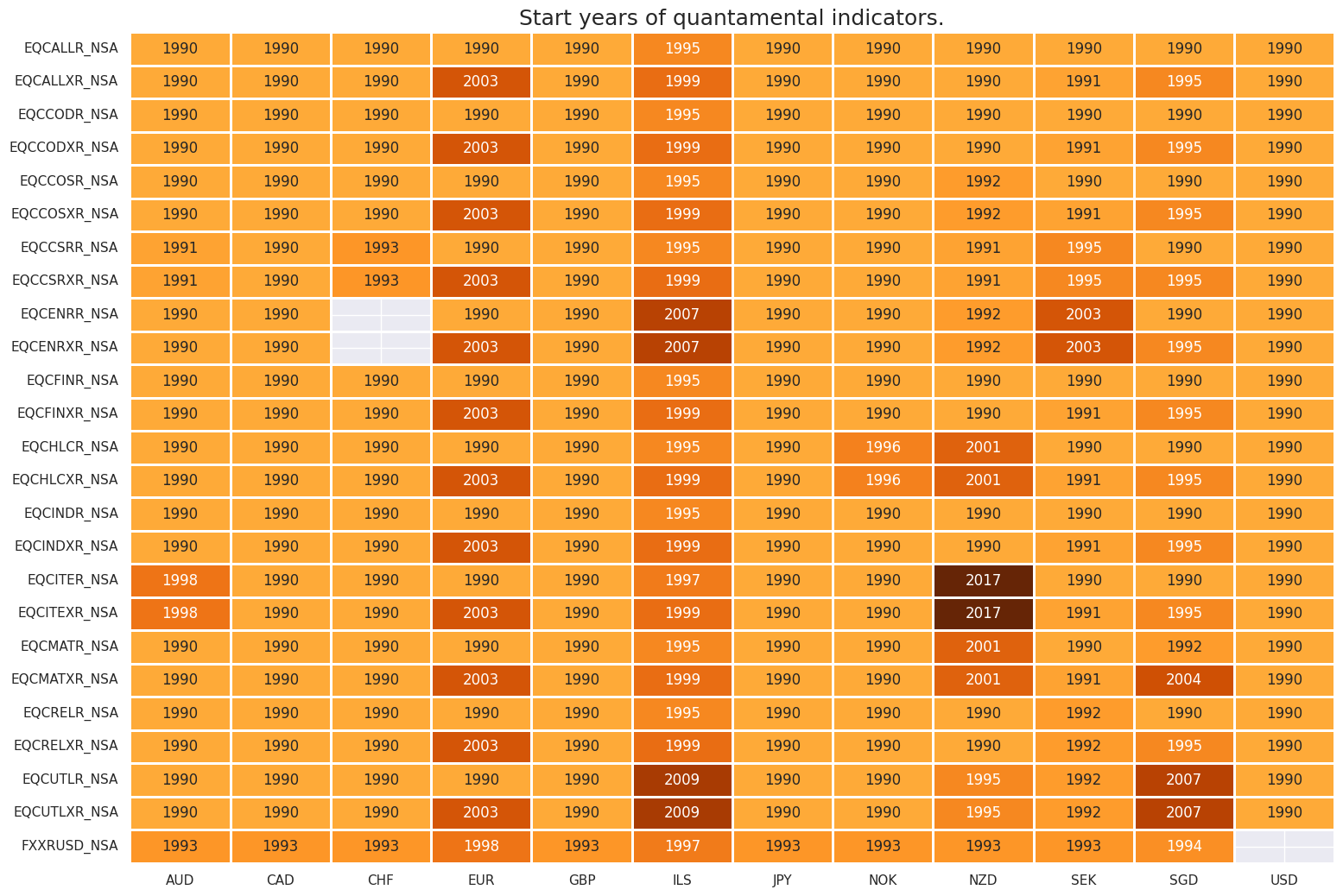
It is important to assess data availability before conducting any analysis. It allows identifying any potential gaps or limitations in the dataset, which can impact the validity and reliability of analysis and ensure that a sufficient number of observations for each selected category and cross-section is available as well as determining the appropriate time periods for analysis.

ecos_xq = list(set(ecos) - set(dict_repl.keys()))
msm.missing_in_df(df, xcats=ecos_xq, cids=cids)

No missing XCATs across DataFrame.
Missing cids for CCSCORE_SA:                ['HKD', 'SGD']
Missing cids for CCSCORE_SA_D3M3ML3:        ['CHF', 'HKD', 'NZD', 'SGD']
Missing cids for CPIC_SA_P1M1ML12:          ['HKD']
Missing cids for CPIC_SJA_P3M3ML3AR:        ['HKD']
Missing cids for EXPORTS_SA_P1M1ML12_3MMA:  ['DEM', 'ESP', 'FRF', 'HKD', 'ITL', 'NLG']
Missing cids for EXPORTS_SA_P6M6ML6AR:      ['DEM', 'ESP', 'FRF', 'HKD', 'ITL', 'NLG']
Missing cids for IP_SA_P1M1ML12_3MMA:       ['HKD']
Missing cids for IP_SA_P3M3ML3AR:           ['HKD']
Missing cids for IP_SA_P6M6ML6AR:           ['HKD']
Missing cids for MBCSCORE_SA:               []
Missing cids for MBCSCORE_SA_D3M3ML3:       ['HKD']
Missing cids for PCREDITBN_SJA_P1M1ML12:    ['DEM', 'ESP', 'FRF', 'HKD', 'ITL', 'NLG']
Missing cids for PPIH_NSA_P1M1ML12:         ['HKD']
Missing cids for PPIH_SA_P3M3ML3AR:         ['HKD']
Missing cids for SBCSCORE_SA:               ['HKD', 'NOK']
Missing cids for SBCSCORE_SA_D3M3ML3:       ['AUD', 'GBP', 'HKD', 'JPY', 'NOK', 'SGD']

msm.check_availability(dfx, xcats=manuf, cids=cids_eqx, missing_recent=False)

msm.check_availability(dfx, xcats=servi+consu, cids=cids_eqx, missing_recent=False)

msm.check_availability(dfx, xcats=cpi+ppi, cids=cids_eqx, missing_recent=False)

msm.check_availability(dfx, xcats=ecox, cids=cids_eqx, missing_recent=False)

msm.check_availability(dfx, xcats=eqrets+fxrets, cids=cids_eqx, missing_recent=False)

Transformations and checks

Features

The linear_composite method from the macrosynergy package, is employed to aggregate the individual category scores into a unified composite indicator. This method offers the flexibility to assign specific weights to each category, which can vary over time.

For global industry indicators we use the respective IVAWGT_SA_1YMA , the share in industrial production or world GDP (USD terms), as concurrent weight.

# Global industry indicators
iris = list(set(manuf + ppi).intersection(ecos_xq))  # industry-related indicators
xcatx = iris
cidx = cids_eqx
sdate = "1990-01-01"

dfa = pd.DataFrame(columns=dfx.columns)
for xcat in xcatx:
    dfaa = msp.linear_composite(
        df=dfx,
        xcats=xcat,
        cids=cidx,
        complete_xcats=False,
        start=sdate,
        weights='IVAWGT_SA_1YMA'
    )
    dfa = msm.update_df(dfa, dfaa)

dfx = msm.update_df(dfx, dfa)

For services and consumption indicator composite we employ as weight 'USDGDPWGT_SA_1YMA' denoting the share in world GDP (USD terms): based on 1-year moving average.

# Global services and consumption indicators

cscs = list(set(servi + consu + cpi).intersection(ecos_xq))
xcatx = cscs
cidx = cids_eqx
sdate = "1990-01-01"

dfa = pd.DataFrame(columns=dfx.columns)
for xcat in xcatx:
    dfaa = msp.linear_composite(
        df=dfx,
        xcats=xcat,
        cids=cidx,
        complete_xcats=False,
        start=sdate,
        weights='USDGDPWGT_SA_1YMA'
    )
    dfa = msm.update_df(dfa, dfaa)

dfx = msm.update_df(dfx, dfa)

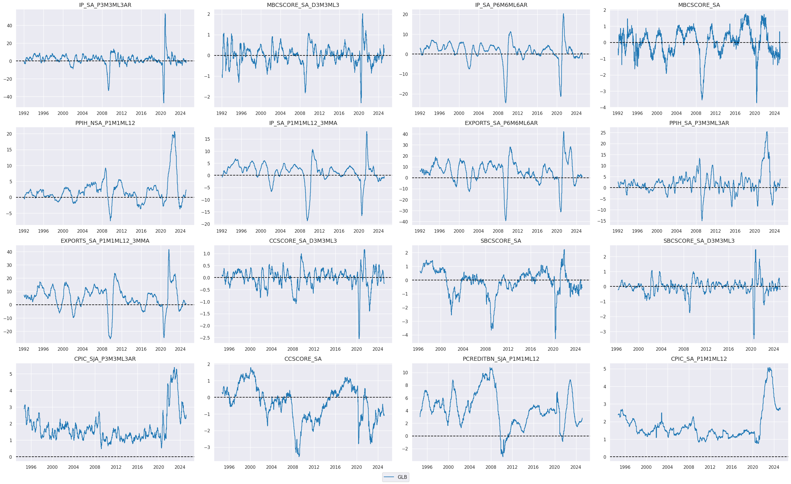
view_timelines() from the macrosynergy package is used to plot the timelines of the created global indicators:

xcatx = iris + cscs
cidx = 'GLB'
start_date = "1990-01-01"

msp.view_timelines(
    dfx,
    xcats=xcatx,
    cids=cidx,
    start=start_date,
    title=None,
    cumsum=False,
    ncol=4,
    same_y=False,
    size=(12, 7),
    all_xticks=True,
    xcat_grid=True,
)

Targets

In addition to the standard sectoral equity returns, we build new return series to be able to analyse the country’s sectoral performance in excess of the local equity market and in excess of the global sector performance.

Cross-sector returns (for all countries)

We compute the sector-specific return vALL in a given region by subtracting from each indicator the equal-weighted average of sector returns of the corresponding cross-section. To do this, we apply the Macrosynergy package method make_relative_category() from the macrosynergy package.

An alternative option would be subtracting the aggregate equity index return EQCALLR_NSA from each of the sectoral returns.

cidx = cids_eqx
dfa = pd.DataFrame(columns=dfx.columns)

for ret in ["R", "XR"]:
    xcatx = [f"EQC{sec}{ret}_NSA" for sec in secs]
    dfaa = msp.make_relative_category(
        df=dfx,
        xcats=xcatx,
        cids=cidx,
        start="1990-01-01",
        basket=None,
        complete_set=False,
        rel_meth="subtract",
        postfix="vALL",
    )
    dfa = msm.update_df(dfa, dfaa)

dfx = msm.update_df(dfx, dfa)

The cross section, CHF, is missing ['EQCENRR_NSA'] from the requested basket. The new basket will be ['EQCCODR_NSA', 'EQCCOSR_NSA', 'EQCCSRR_NSA', 'EQCFINR_NSA', 'EQCHLCR_NSA', 'EQCINDR_NSA', 'EQCITER_NSA', 'EQCMATR_NSA', 'EQCRELR_NSA', 'EQCUTLR_NSA'].
The cross section, CHF, is missing ['EQCENRXR_NSA'] from the requested basket. The new basket will be ['EQCCODXR_NSA', 'EQCCOSXR_NSA', 'EQCCSRXR_NSA', 'EQCFINXR_NSA', 'EQCHLCXR_NSA', 'EQCINDXR_NSA', 'EQCITEXR_NSA', 'EQCMATXR_NSA', 'EQCRELXR_NSA', 'EQCUTLXR_NSA'].

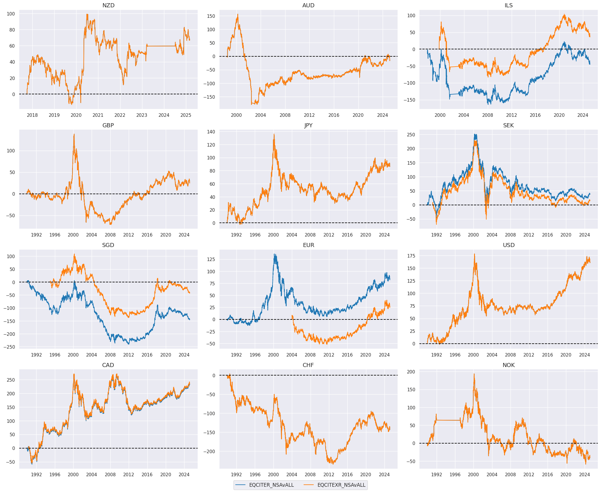
Since local returns are calculated based on the same funding costs across sectors, relative cash and excess returns are equal, except for different starting points of history. view_timelines() from the macrosynergy package is used to plot the timelines of the selected sector return (below - Information tech):

sec = "ITE"
xcatx = [
    f"EQC{sec}R_NSAvALL", 
    f"EQC{sec}XR_NSAvALL"
]
cidx = cids_eqx
start_date = "1990-01-01"

msp.view_timelines(
    dfx,
    xcats=xcatx,
    cids=cidx,
    start=start_date,
    cumsum=True,
    ncol=3,
    same_y=False,
    size=(12, 7),
    all_xticks=True,
    xcat_grid=False,
)

Intra-sector cross-country relative returns

We also compute the country-specific return for a given sector, as we want to analyse its relative performance beyond what happens to that basket of stocks globally.

To do this, we first have to incorporate local currency returns vs USD so that the relative performance of the sector across regions can be evaluated without worrying of the denominator. We use the package’s method panel_calculator() to aggregate local currency equity excess returns, local currency FX excess returns, and USD funding rate.

# Proxy USD cash returns

cidx = list(set(cids_eqx) - {'USD'})
calcs = []

for sec in secx:
    calcs += [f"EQC{sec}RUSD_NSA = EQC{sec}XR_NSA + FXXRUSD_NSA + iUSD_EQCALLR_NSA - iUSD_EQCALLXR_NSA"]

dfa = msp.panel_calculator(df=dfx, calcs=calcs, cids=cids_eqx)
dfx = msm.update_df(dfx, dfa)

# Add renamed USD cash returns for panel consistency

filt = dfx["cid"].isin(['USD']) & dfx["xcat"].str.contains(r'EQC...R_NSA$', regex=True)
dfa = dfx[filt]
dfa['xcat'] = dfa['xcat'].str.replace('R_NSA', 'RUSD_NSA')
dfx = msm.update_df(dfx, dfa)

Similar to what done above, we compute the sector relative USD return using the method make_relative_value() . The new series is assigned postfix vGLB

usrets = ["EQC" + sec + "RUSD_NSA" for sec in secx]
xcatx = usrets
cidx = cids_eqx

dfa = msp.make_relative_value(
    dfx,
    xcats=xcatx,
    cids=cidx,
    start="1990-01-01",
    rel_meth="subtract",
    postfix="vGLB",
)

dfx = msm.update_df(dfx, dfa)

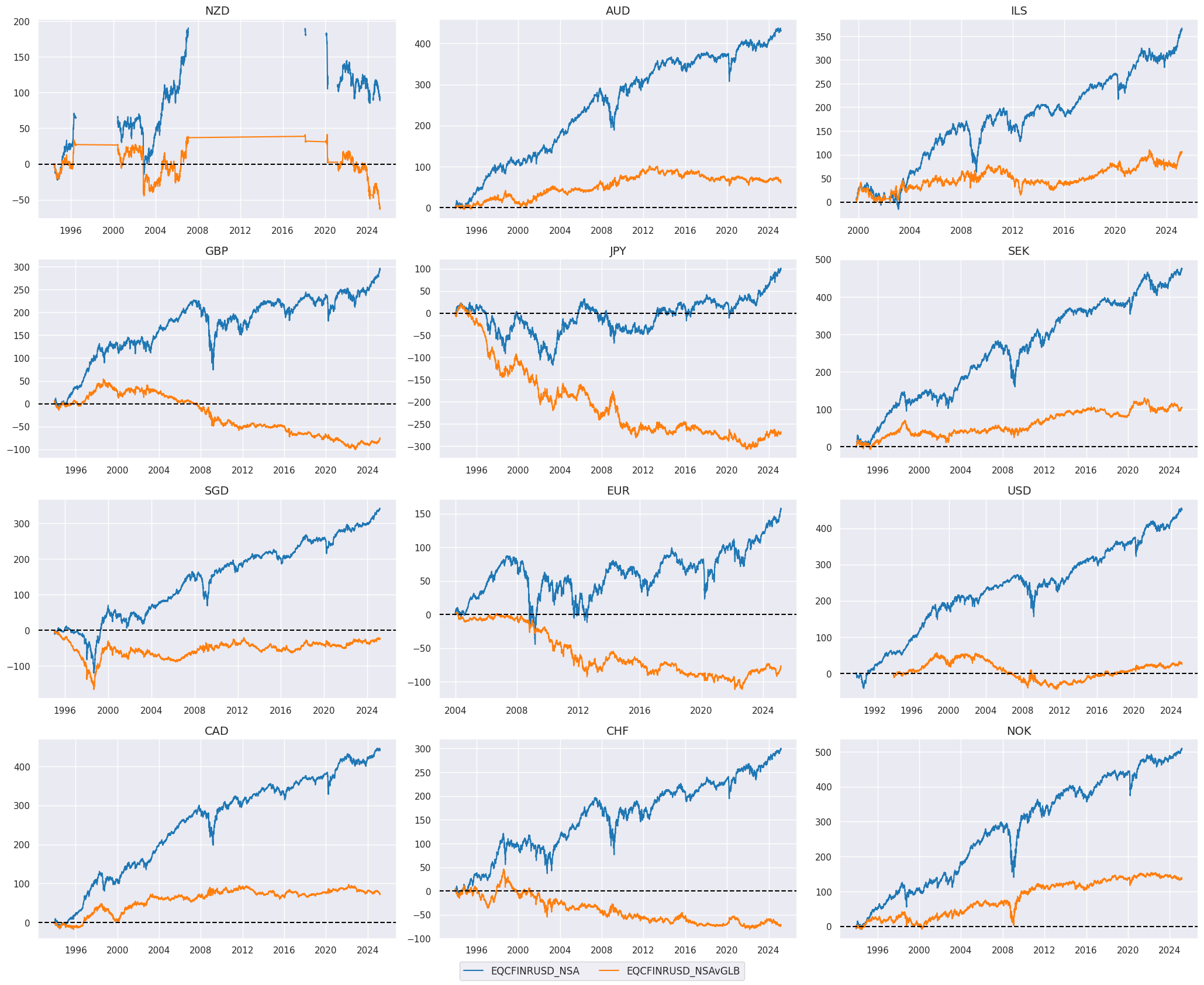
view_timelines() from the macrosynergy package is used to plot the timeline of the country-specific relative return vGLB for a chosen sector (Financials in the example below) across cross-sections:

sec = "FIN"
xcatx = [f"EQC{sec}RUSD_NSA", f"EQC{sec}RUSD_NSAvGLB"]
cidx = cids_eqx
start_date = "1990-01-01"

msp.view_timelines(
    dfx,
    xcats=xcatx,
    cids=cidx,
    start=start_date,
    cumsum=True,
    ncol=3,
    same_y=False,
    size=(12, 7),
    all_xticks=True,
    xcat_grid=False,
)

Value checks

The notebook evaluates the predictive relations of quantamental indicators (standard and linear composite indicators) by means of panel regression, i.e., the joint consideration of macro trends and relative equity returns over a set of cross sections (currency areas or sectors). The notebook computes various metrics and ratios, including:

• Correlation: Measures the relationship between meaningful economic trends and consequent equity cross-sector and cross-country returns.

• Accuracy Metrics: These metrics assess the accuracy of the selectged indicators in predicting market movements. Common accuracy metrics include accuracy rate, balanced accuracy, precision etc.

The Value checks section is split into two parts:

The first part looks at allocation across sectors, within the same currency area. For example, some sectors are naturally more sensitive to growth, while others are more susceptible to financial conditions or inflation headwinds. This part considers a few plausible hypothesis:

• strong excess export growth positively predicts the relative performance of the energy sector,

• positive business sentiment in services surveys predicts good subsequent business results in key services sectors, i.e., health care and utilities,

• High consumer confidence predicts real estate outperformance,

• High inflation predicts real estate underperformance.

The second part looks at the allocation across currency areas, particularly within the same sector. For real money investors such allocations typically involve both currency and pure equity risk. Relative economic trends, such as growth differentials, matter if they have significant predictive power for the joint currency or equity portion of the return and if cross-country divergences are common and sizable. This part considers a few plausible hypotheses:

• relative export growth positively predicts relative cross-country equity performance across various sectors,

• relative changes in business confidence score positively predict relative returns for industrial stocks as well as overall equity indices that include all sectors,

• a steeper real yield curve bodes for better returns for financial sector.

Cross-sector allocations

JPMaQS quantamental indicators can be a relevant guide to building sectoral rotational strategies in the equity space. Here we provide a glance at some of the relationships that link pure macroeconomic trends to the sector outperformance vs the local region equity index. As we show, value can be extracted both from forward-looking metrics such as consumer, manufacturing, and service survey score as well as from point-in-time backward-looking measures of realised economic activity.

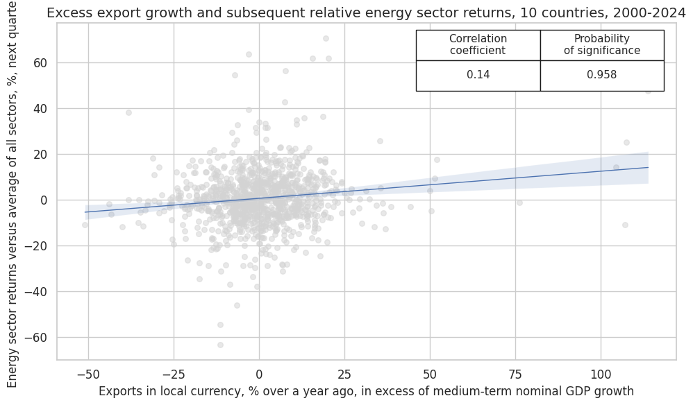
Export growth predicts energy sector outperformance

Deviation of production prices and volumes, as well as exports, above their natural growth trend, provides a strong case for global and local real growth, which is generally associated with positive energy demand growth. This creates the base for the energy equity sector’s relative performance.

Specs and panel tests

Here, we create plausible excess growth indicator groups using panel_calculator() method. For example

• EXPORTS_SA_P6M6ML6AR_XNGDP denotes excess export growth,

• PPIH_NSA_P1M1ML12_XIT is excess inflation based on producer price inflation

cidx = cids_eqx
calcs = []

ips = ["IP_SA_P3M3ML3AR", "IP_SA_P6M6ML6AR", "IP_SA_P1M1ML12_3MMA"]
for ip in ips:
    calcs += [f"{ip}_XGDP = {ip} - RGDP_SA_P1Q1QL4_20QMM"]
 #   calcs += [f"{ip}_XIGDP = {ip} - INTRGDP_NSA_P1M1ML12_3MMA"]

xps = ["EXPORTS_SA_P6M6ML6AR", "EXPORTS_SA_P1M1ML12_3MMA"]
for xp in xps:
    calcs += [f"{xp}_XNGDP = {xp} - RGDP_SA_P1Q1QL4_20QMM - INFTEFF_NSA"]

pps = ["PPIH_NSA_P1M1ML12", "PPIH_SA_P3M3ML3AR"]
for pp in pps:
    calcs += [f"{pp}_XIT = {pp} - INFTEFF_NSA"]

dfa = msp.panel_calculator(df=dfx, calcs=calcs, cids=cids_eqx)
dfx = msm.update_df(dfx, dfa)

cidx = cids_eqx
sigs = [
    "EXPORTS_SA_P1M1ML12_3MMA_XNGDP",
    "EXPORTS_SA_P6M6ML6AR_XNGDP",
    "IP_SA_P1M1ML12_3MMA_XGDP",
    "PPIH_NSA_P1M1ML12_XIT",
]
rets = ["EQCENRR_NSAvALL"]
start = "2000-01-01"

dict_exen = {
    "sigs": sigs,
    "rets": rets,
    "cidx": cidx,
    "start": start,
    "black": None,
    "srr": None,
    "pnls": None,
}

CategoryRelations() function is used for quick visualization and analysis of two categories, in particular,

• Excess export growth EXPORTS_SA_P1M1ML12_3MMA_XNGDP , derived earlier, and

• subsequent energy sector returns versus the average of all sectors EQCENRR_NSAvALL

The .reg_scatter() method is convenient for visualizing the relationship between two categories, including the strength of the linear association and any potential outliers. It includes a regression line with a 95% confidence interval, which can help assess the significance of the relationship. The analysis is done on a quarterly basis.

dix = dict_exen

sig = dix["sigs"][0]
ret = dix["rets"][0]
cidx = dix["cidx"]
blax = dix["black"]
start = dix["start"]

crx_mat = msp.CategoryRelations(
    dfx,
    xcats=[sig, ret],
    cids=cidx,
    freq="Q",
    lag=1,
    xcat_aggs=["last", "sum"],
    start=start,
    blacklist=None,
)
crx_mat.reg_scatter(
    labels=False,
    coef_box="upper right",
    xlab="Exports in local currency, % over a year ago, in excess of medium-term nominal GDP growth",
    ylab="Energy sector returns versus average of all sectors, %, next quarter",
    title="Excess export growth and subsequent relative energy sector returns, 10 countries, 2000-2024",
    size=(10, 6),
    prob_est="map",
)

EQCENRR_NSAvALL misses: ['CHF'].

Accuracy and correlation check

SignalReturnRelations() function from the macrosynergy package analyses and compares the relationships between the chosen signals and the panel of subsequent returns. There is no regression analysis involved, rather the sign of the signal is used for predicting the sign of the target.

dix = dict_exen

sigs = dix["sigs"]
rets = dix["rets"]
cidx = dix["cidx"]
blax = dix["black"]
start = dix["start"]

srr = mss.SignalReturnRelations(
    dfx,
    cids=cidx,
    sigs=sigs,
    rets=rets,
    freqs="M",
    start=start,
    blacklist=blax,
)

dix["srr"] = srr

dix = dict_exen
srrx = dix["srr"]
xms = ["accuracy", "bal_accuracy", "pos_sigr", "pos_retr", "pearson", "pearson_pval", "kendall", "kendall_pval"]

The summary table below gives a short high-level snapshot of the strength and stability of the main signal and alternative signal relation.

display(srrx.signals_table().sort_index().astype("float").round(3)[xms])

				accuracy	bal_accuracy	pos_sigr	pos_retr	pearson	pearson_pval	kendall	kendall_pval
Return	Signal	Frequency	Aggregation
EQCENRR_NSAvALL	EXPORTS_SA_P1M1ML12_3MMA_XNGDP	M	last	0.536	0.536	0.491	0.493	0.105	0.000	0.055	0.000
	EXPORTS_SA_P6M6ML6AR_XNGDP	M	last	0.518	0.518	0.498	0.493	0.085	0.000	0.042	0.000
	IP_SA_P1M1ML12_3MMA_XGDP	M	last	0.522	0.522	0.361	0.494	0.055	0.002	0.031	0.010
	PPIH_NSA_P1M1ML12_XIT	M	last	0.524	0.524	0.507	0.493	0.095	0.000	0.039	0.001

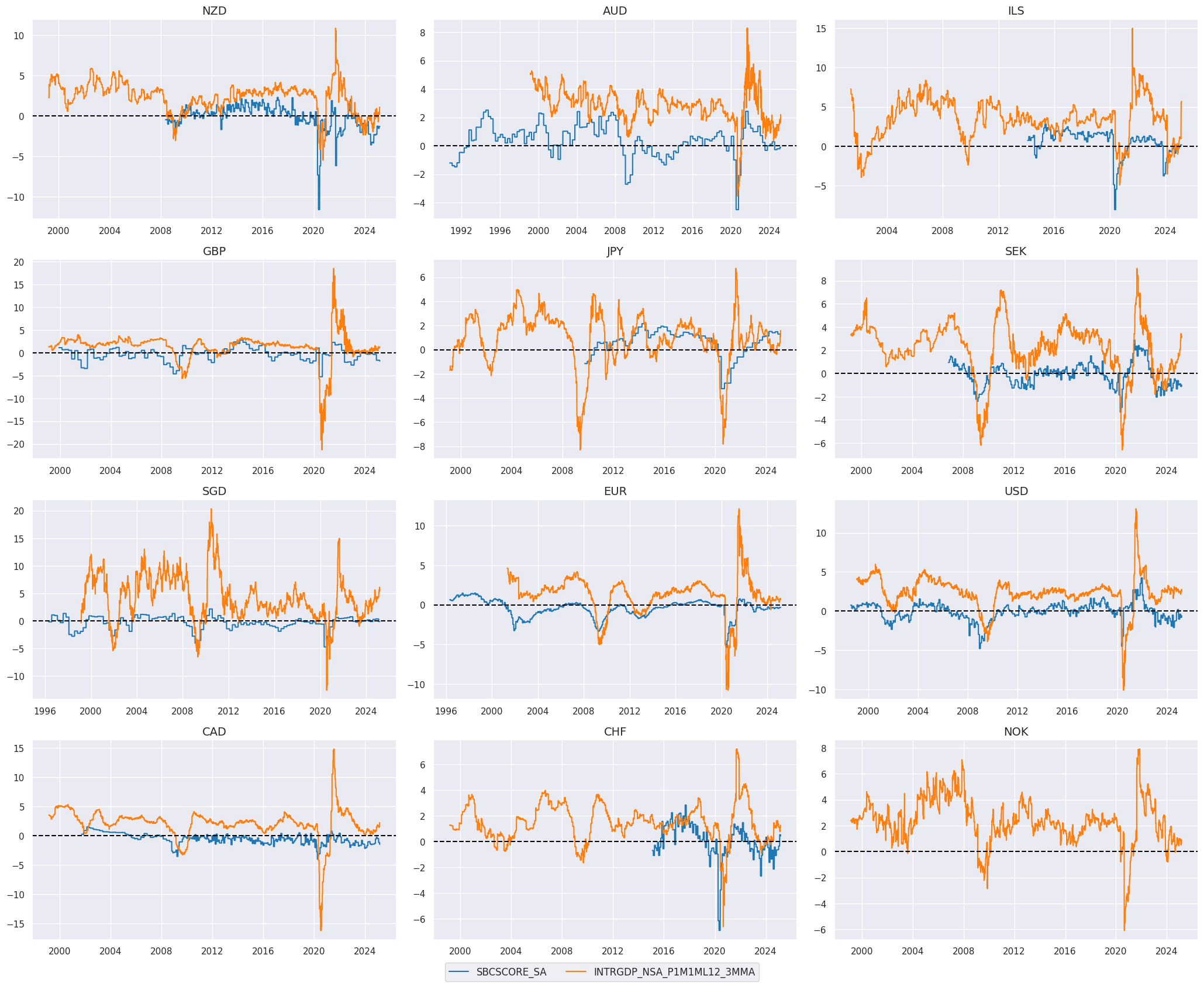
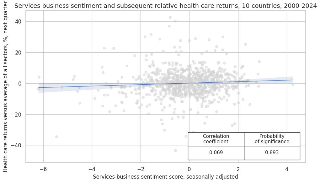
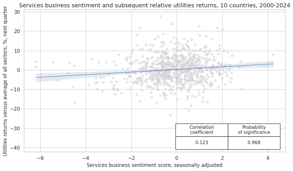
High services sentiment predicts outperformance of health care and utilities stocks

The service industry expectations are positively correlated with measures of economic growth. As we show below, the level of service sentiment and higher frequency nowcasted real growth rates go hand in hand. The quantamental indicators are relatively forward-looking measurements, with little release lag so accurately reflect the state of the economy.

This is helpful in identifying turning points for the relative performance of more defensive, less cyclical sectors such as utilities and healthcare stocks. These show a strong positive relationship with the selected quantamental indicators over quarterly frequency.

xcatx = ["SBCSCORE_SA", "INTRGDP_NSA_P1M1ML12_3MMA"]
cidx = cids_eqx
start_date = "1990-01-01"

msp.view_timelines(
    dfx,
    xcats=xcatx,
    cids=cidx,
    start=start_date,
    cumsum=False,
    ncol=3,
    same_y=False,
    size=(12, 7),
    all_xticks=True,
    xcat_grid=False,
)

Specs and panel tests

cidx = cids_eqx
sigs = ["SBCSCORE_SA", "SBCSCORE_SA_D3M3ML3"]
rets = ["EQCHLCR_NSAvALL", "EQCUTLR_NSAvALL"]
start = "2000-01-01"

dict_sshu = {
    "sigs": sigs,
    "rets": rets,
    "cidx": cidx,
    "start": start,
    "black": None,
    "srr": None,
    "pnls": None,
}

CategoryRelations() function is used for quick visualization and analysis of two categories, in particular,

• Services confidence scores SBCSCORE_SA , and

• subsequent relative health care returns EQCHLCR_NSAvALL

The .reg_scatter() method is convenient for visualizing the relationship between two categories, including the strength of the linear association and any potential outliers. It includes a regression line with a 95% confidence interval, which can help assess the significance of the relationship. The analysis is done on a quarterly basis.

dix = dict_sshu

sig = dix["sigs"][0]
ret = dix["rets"][0]
cidx = dix["cidx"]
blax = dix["black"]
start = dix["start"]

crx_mat = msp.CategoryRelations(
    dfx,
    xcats=[sig, ret],
    cids=cidx,
    freq="Q",
    lag=1,
    xcat_aggs=["last", "sum"],
    start=start,
    blacklist=None,
    xcat_trims=[10, 50]  # adjust for extreme > 10 SD outlier
)
crx_mat.reg_scatter(
    labels=False,
    coef_box="lower right",
    xlab="Services business sentiment score, seasonally adjusted",
    ylab="Health care returns versus average of all sectors, %, next quarter",
    title="Services business sentiment and subsequent relative health care returns, 10 countries, 2000-2024",
    size=(10, 6),
    prob_est="map",
)

SBCSCORE_SA misses: ['NOK'].

CategoryRelations() function is used for quick visualization and analysis of two categories. Her it analyses

• services confidence scores SBCSCORE_SA , and

• subsequent utilities returns versus average of all sectors EQCHLCR_NSAvALL

The .reg_scatter() method is convenient for visualizing the relationship between two categories, including the strength of the linear association and any potential outliers. It includes a regression line with a 95% confidence interval, which can help assess the significance of the relationship. The analysis is done on a quarterly basis.

dix = dict_sshu

sig = dix["sigs"][0]
ret = dix["rets"][1]
cidx = dix["cidx"]
blax = dix["black"]
start = dix["start"]

crx_mat = msp.CategoryRelations(
    dfx,
    xcats=[sig, ret],
    cids=cidx,
    freq="Q",
    lag=1,
    xcat_aggs=["last", "sum"],
    start=start,
    blacklist=None,
    xcat_trims=[10, 50]  # adjust for extreme > 10 SD outlier
)
crx_mat.reg_scatter(
    labels=False,
    coef_box="lower right",
    xlab="Services business sentiment score, seasonally adjusted",
    ylab="Utilities returns versus average of all sectors, %, next quarter",
    title="Services business sentiment and subsequent relative utilities returns, 10 countries, 2000-2024",
    size=(10, 6),
    prob_est="map",
)

SBCSCORE_SA misses: ['NOK'].

Accuracy and correlation check

SignalReturnRelations() function from the macrosynergy package analyses and compares the relationships between the chosen signals and the panel of subsequent returns. There is no regression analysis involved, rather the sign of the signal is used for predicting the sign of the target.

dix = dict_sshu

sigs = dix["sigs"]
rets = dix["rets"]
cidx = dix["cidx"]
blax = dix["black"]
start = dix["start"]

srr = mss.SignalReturnRelations(
    df=dfx,
    cids=cidx,
    sigs=sigs,
    rets=rets,
    freqs="M",
    start="1995-01-01",
)

mrt = srr.multiple_relations_table(rets=rets, xcats=sigs)

display(mrt.sort_index().astype("float").round(3)[xms])

				accuracy	bal_accuracy	pos_sigr	pos_retr	pearson	pearson_pval	kendall	kendall_pval
Return	Signal	Frequency	Aggregation
EQCHLCR_NSAvALL	SBCSCORE_SA	M	last	0.510	0.510	0.513	0.507	0.026	0.174	0.024	0.056
	SBCSCORE_SA_D3M3ML3	M	last	0.500	0.500	0.500	0.505	0.003	0.887	-0.005	0.716
EQCUTLR_NSAvALL	SBCSCORE_SA	M	last	0.531	0.531	0.502	0.511	0.054	0.008	0.043	0.002
	SBCSCORE_SA_D3M3ML3	M	last	0.514	0.514	0.503	0.509	0.012	0.573	0.012	0.370

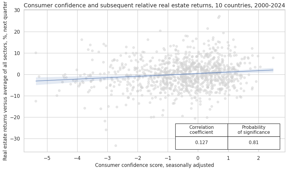
High consumer confidence predicts real estate outperformance

Here the idea is that strong household sentiment fosters particular demand for residential real estate. Moreover, circumstances that support household confidence, such as low inflation and low real interest rates also support demand for housing.

Specs and panel test

cidx = cids_eqx
sigs = ["CCSCORE_SA", "CCSCORE_SA_D3M3ML3"]
rets = ["EQCRELR_NSAvALL"]
start = "2000-01-01"

dict_ccre = {
    "sigs": sigs,
    "rets": rets,
    "cidx": cidx,
    "start": start,
    "black": None,
    "srr": None,
    "pnls": None,
}

CategoryRelations() function is used for quick visualization and analysis of two categories. Her it analyses

• consumer confidence scores CCSCORE_SA , and

• subsequent relative real estate returns EQCRELR_NSAvALL

The .reg_scatter() method is convenient for visualizing the relationship between two categories, including the strength of the linear association and any potential outliers. It includes a regression line with a 95% confidence interval, which can help assess the significance of the relationship. The analysis is done on a quarterly basis.

dix = dict_ccre

sig = dix["sigs"][0]
ret = dix["rets"][0]
cidx = dix["cidx"]
blax = dix["black"]
start = dix["start"]

crx_mat = msp.CategoryRelations(
    dfx,
    xcats=[sig, ret],
    cids=cidx,
    freq="Q",
    lag=1,
    xcat_aggs=["last", "sum"],
    start=start,
    blacklist=None,
)
crx_mat.reg_scatter(
    labels=False,
    coef_box="lower right",
    xlab="Consumer confidence score, seasonally adjusted",
    ylab="Real estate returns versus average of all sectors, %, next quarter",
    title="Consumer confidence and subsequent relative real estate returns, 10 countries, 2000-2024",
    size=(10, 6),
    prob_est="map",
)

CCSCORE_SA misses: ['SGD'].

Accuracy and correlation check

SignalReturnRelations() function from the macrosynergy package analyses and compares the relationships between the chosen signals and the panel of subsequent returns. There is no regression analysis involved, rather the sign of the signal is used for predicting the sign of the target.

dix = dict_ccre

sigs = dix["sigs"]
rets = dix["rets"]
cidx = dix["cidx"]
blax = dix["black"]
start = dix["start"]

srr = mss.SignalReturnRelations(
    df=dfx,
    cids=cidx,
    sigs=sigs,
    rets=rets,
    freqs="M",
    start="1995-01-01",
)

display(mrt.sort_index().astype("float").round(3)[xms])

				accuracy	bal_accuracy	pos_sigr	pos_retr	pearson	pearson_pval	kendall	kendall_pval
Return	Signal	Frequency	Aggregation
EQCHLCR_NSAvALL	SBCSCORE_SA	M	last	0.510	0.510	0.513	0.507	0.026	0.174	0.024	0.056
	SBCSCORE_SA_D3M3ML3	M	last	0.500	0.500	0.500	0.505	0.003	0.887	-0.005	0.716
EQCUTLR_NSAvALL	SBCSCORE_SA	M	last	0.531	0.531	0.502	0.511	0.054	0.008	0.043	0.002
	SBCSCORE_SA_D3M3ML3	M	last	0.514	0.514	0.503	0.509	0.012	0.573	0.012	0.370

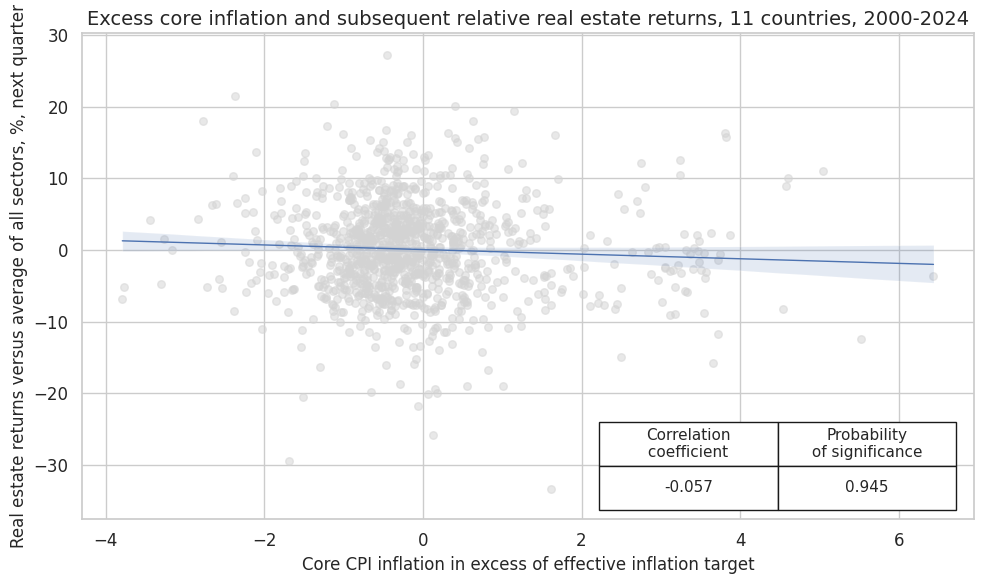
High inflation predicts real estate underperformance

Real estate equity sector includes both REITs businesses and real estate development companies. Even if the economic nature of the activity is slightly different, the two sets of companies operate with high leverage and would be naturally affected by changes in interest rates. The excess core inflation indicators are a strong predictor of future rates movement, therefore they are applicable in this case.

Specs and panel tests

for cpi in ["CPIC_SA_P1M1ML12", "CPIC_SJA_P3M3ML3AR"]:
    calcs += [f"{cpi}_XIT = {cpi} - INFTEFF_NSA"]
dfa = msp.panel_calculator(df=dfx, calcs=calcs, cids=cids_eqx)
dfx = msm.update_df(dfx, dfa)

cidx = cids_eqx
sigs = ["CPIC_SA_P1M1ML12_XIT", "CPIC_SJA_P3M3ML3AR_XIT"]
rets = ["EQCRELR_NSAvALL"]
start = "2000-01-01"

dict_cpre = {
    "sigs": sigs,
    "rets": rets,
    "cidx": cidx,
    "start": start,
    "black": None,
    "srr": None,
    "pnls": None,
}

CategoryRelations() function is used for quick visualization and analysis of two categories. Her it analyses

• Core CPI inflation in excess of effective inflation target CPIC_SA_P1M1ML12_XIT , and

• Real estate returns versus average of all sectors EQCRELR_NSAvALL

The .reg_scatter() method is convenient for visualizing the relationship between two categories, including the strength of the linear association and any potential outliers. It includes a regression line with a 95% confidence interval, which can help assess the significance of the relationship. The analysis is done on a quarterly basis.

dix = dict_cpre

sig = dix["sigs"][0]
ret = dix["rets"][0]
cidx = dix["cidx"]
blax = dix["black"]
start = dix["start"]

crx_mat = msp.CategoryRelations(
    dfx,
    xcats=[sig, ret],
    cids=cidx,
    freq="Q",
    lag=1,
    xcat_aggs=["last", "sum"],
    start=start,
    blacklist=None,
)
crx_mat.reg_scatter(
    labels=False,
    coef_box="lower right",
    xlab="Core CPI inflation in excess of effective inflation target",
    ylab="Real estate returns versus average of all sectors, %, next quarter",
    title="Excess core inflation and subsequent relative real estate returns, 11 countries, 2000-2024",
    size=(10, 6),
    prob_est="pool",
)

Accuracy and correlation check

SignalReturnRelations() function from the macrosynergy package analyses and compares the relationships between the chosen signals and the panel of subsequent returns. There is no regression analysis involved, rather the sign of the signal is used for predicting the sign of the target.

dix = dict_cpre

sigs = dix["sigs"]
rets = dix["rets"]
cidx = dix["cidx"]
blax = dix["black"]
start = dix["start"]

srr = mss.SignalReturnRelations(
    df=dfx,
    cids=cidx,
    sigs=sigs,
    rets=rets,
    freqs="M",
    start="1995-01-01",
)

mrt = srr.multiple_relations_table(rets=rets, xcats=sigs)

display(mrt.sort_index().astype("float").round(3)[xms])

				accuracy	bal_accuracy	pos_sigr	pos_retr	pearson	pearson_pval	kendall	kendall_pval
Return	Signal	Frequency	Aggregation
EQCRELR_NSAvALL	CPIC_SA_P1M1ML12_XIT	M	last	0.500	0.497	0.325	0.494	-0.034	0.041	-0.010	0.379
	CPIC_SJA_P3M3ML3AR_XIT	M	last	0.499	0.498	0.398	0.494	-0.040	0.017	-0.006	0.602

Intra-sector cross-country allocations

Another potential use case of JPMaQS quantamental indicators is presented by cross-country equity allocation for given sectors. In similar fashion to what built above, we link both backward and forward looking macroeconomic variables to relative equity performance.

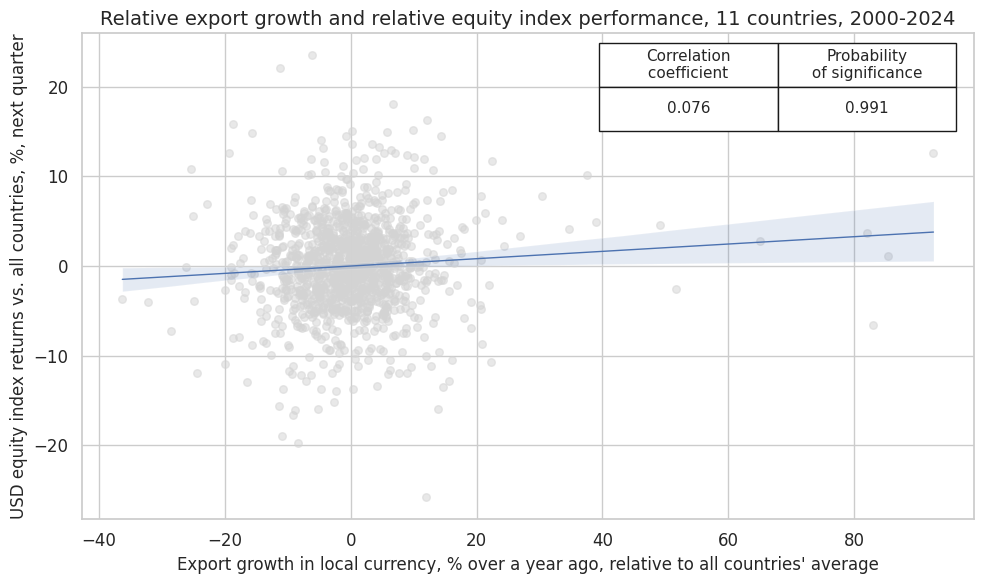
Stronger export growth predicts country outperformance, marketwide and for some sectors

With a similar approach to the previous case, relative positive/negative export trends across countries are a manifestation of improving / degrading relative conditions of the local economy. This provides the basis for relative trades of USD-denominated local equity indices and more cyclical sectors such as energy and industrials.

Specs and panel tests

cidx = cids_eqx
xcatx = ["EXPORTS_SA_P6M6ML6AR", "EXPORTS_SA_P1M1ML12_3MMA"]

dfa = msp.make_relative_value(
    dfx,
    xcats=xcatx,
    cids=cidx,
    start="1990-01-01",
    rel_meth="subtract",
    postfix="vGLB",
)

dfx = msm.update_df(dfx, dfa)

cidx = cids_eqx
sigs = [
    "EXPORTS_SA_P1M1ML12_3MMAvGLB",
    "EXPORTS_SA_P6M6ML6ARvGLB",
]
rets = ["EQCALLRUSD_NSAvGLB", "EQCENRRUSD_NSAvGLB", "EQCINDRUSD_NSAvGLB"]
start = "2000-01-01"

dict_exxc = {
    "sigs": sigs,
    "rets": rets,
    "cidx": cidx,
    "start": start,
    "black": None,
    "srr": None,
    "pnls": None,
}

CategoryRelations() function is used for quick visualization and analysis of two categories. Here it analyses

• Export growth in local currency, % over a year ago, relative to all countries’ average EXPORTS_SA_P1M1ML12_3MMAvGLB , and

• subsequent USD equity index returns vs. all countries EQCALLRUSD_NSAvGLB

The .reg_scatter() method is convenient for visualizing the relationship between two categories, including the strength of the linear association and any potential outliers. It includes a regression line with a 95% confidence interval, which can help assess the significance of the relationship. The analysis is done on a quarterly basis.

dix = dict_exxc

sig = dix["sigs"][0]
ret = dix["rets"][0]
cidx = dix["cidx"]
blax = dix["black"]
start = dix["start"]

crx_mat = msp.CategoryRelations(
    dfx,
    xcats=[sig, ret],
    cids=cidx,
    freq="Q",
    lag=1,
    xcat_aggs=["last", "sum"],
    start=start,
    blacklist=None,
)
crx_mat.reg_scatter(
    labels=False,
    coef_box="upper right",
    xlab="Export growth in local currency, % over a year ago, relative to all countries' average",
    ylab="USD equity index returns vs. all countries, %, next quarter",
    title="Relative export growth and relative equity index performance, 11 countries, 2000-2024",
    size=(10, 6),
    prob_est="map",
)

Accuracy and correlation check

SignalReturnRelations() function from the macrosynergy package analyses and compares the relationships between the chosen signals and the panel of subsequent returns. There is no regression analysis involved, rather the sign of the signal is used for predicting the sign of the target.

dix = dict_exxc

sigs = dix["sigs"]
rets = dix["rets"]
cidx = dix["cidx"]
blax = dix["black"]
start = dix["start"]

srr = mss.SignalReturnRelations(
    df=dfx,
    cids=cidx,
    sigs=sigs,
    rets=rets,
    freqs="M",
    start="1995-01-01",
)

mrt = srr.multiple_relations_table(rets=rets, xcats=sigs)

display(mrt.sort_index().astype("float").round(3)[xms])

				accuracy	bal_accuracy	pos_sigr	pos_retr	pearson	pearson_pval	kendall	kendall_pval
Return	Signal	Frequency	Aggregation
EQCALLRUSD_NSAvGLB	EXPORTS_SA_P1M1ML12_3MMAvGLB	M	last	0.511	0.511	0.470	0.499	0.040	0.011	0.025	0.018
	EXPORTS_SA_P6M6ML6ARvGLB	M	last	0.499	0.499	0.462	0.499	0.036	0.022	0.015	0.142
EQCENRRUSD_NSAvGLB	EXPORTS_SA_P1M1ML12_3MMAvGLB	M	last	0.510	0.510	0.467	0.493	0.034	0.045	0.017	0.134
	EXPORTS_SA_P6M6ML6ARvGLB	M	last	0.510	0.509	0.465	0.493	0.031	0.074	0.024	0.038
EQCINDRUSD_NSAvGLB	EXPORTS_SA_P1M1ML12_3MMAvGLB	M	last	0.516	0.517	0.470	0.507	0.025	0.108	0.018	0.080
	EXPORTS_SA_P6M6ML6ARvGLB	M	last	0.507	0.507	0.462	0.507	0.025	0.109	0.011	0.276

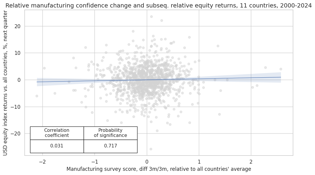
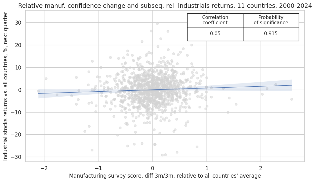
Manufacturing confidence changes predict country outperformance, marketwide and for many sectors

Relative changes in manufacturing business confidence scores should positively predict the relative performance of manufacturing businesses across countries and, by extension, the relative performance of equity returns for the industrial sector and maybe even the overall business sector.

Specs and panel tests

Here we calculate the relative value of manufacturing confidence scores and give them postfix vGLB to indicate “versus Global Benchmark”.

cidx = cids_eqx
xcatx = ["MBCSCORE_SA_D3M3ML3", "MBCSCORE_SA"]

dfa = msp.make_relative_value(
    dfx,
    xcats=xcatx,
    cids=cidx,
    start="1990-01-01",
    rel_meth="subtract",
    postfix="vGLB",
)

dfx = msm.update_df(dfx, dfa)

cidx = cids_eqx
sigs = [
    "MBCSCORE_SA_D3M3ML3vGLB",
    "MBCSCORE_SAvGLB",
]
rets = [
    "EQCALLRUSD_NSAvGLB",
    "EQCCSRRUSD_NSAvGLB",
    "EQCCOSRUSD_NSAvGLB",
    "EQCINDRUSD_NSAvGLB",
]
start = "2000-01-01"

dict_mcxc = {
    "sigs": sigs,
    "rets": rets,
    "cidx": cidx,
    "start": start,
    "black": None,
    "srr": None,
    "pnls": None,
}

CategoryRelations() function is used for quick visualization and analysis of two categories, in particular,

• Relative manufacturing survey score MBCSCORE_SA_D3M3ML3vGLB , and

• subsequent relative equity returns EQCALLRUSD_NSAvGLB

The .reg_scatter() method is convenient for visualizing the relationship between two categories, including the strength of the linear association and any potential outliers. It includes a regression line with a 95% confidence interval, which can help assess the significance of the relationship. The analysis is done on a quarterly basis.

dix = dict_mcxc

sig = dix["sigs"][0]
ret = dix["rets"][0]
cidx = dix["cidx"]
blax = dix["black"]
start = dix["start"]

crx_mat = msp.CategoryRelations(
    dfx,
    xcats=[sig, ret],
    cids=cidx,
    freq="Q",
    lag=1,
    xcat_aggs=["last", "sum"],
    start=start,
    blacklist=None,
)
crx_mat.reg_scatter(
    labels=False,
    coef_box="lower left",
    xlab="Manufacturing survey score, diff 3m/3m, relative to all countries' average",
    ylab="USD equity index returns vs. all countries, %, next quarter",
    title="Relative manufacturing confidence change and subseq. relative equity returns, 11 countries, 2000-2024",
    size=(10, 6),
    prob_est="map",
)

dix = dict_mcxc

sig = dix["sigs"][0]
ret = dix["rets"][3]
cidx = dix["cidx"]
blax = dix["black"]
start = dix["start"]

crx_mat = msp.CategoryRelations(
    dfx,
    xcats=[sig, ret],
    cids=cidx,
    freq="Q",
    lag=1,
    xcat_aggs=["last", "sum"],
    start=start,
    blacklist=None,
)
crx_mat.reg_scatter(
    labels=False,
    coef_box="upper right",
    xlab="Manufacturing survey score, diff 3m/3m, relative to all countries' average",
    ylab="Industrial stocks returns vs. all countries, %, next quarter",
    title="Relative manuf. confidence change and subseq. rel. industrials returns, 11 countries, 2000-2024",
    size=(10, 6),
    prob_est="map",
)

Accuracy and correlation check

SignalReturnRelations() function from the macrosynergy package analyses and compares the relationships between the chosen signals and the panel of subsequent returns. There is no regression analysis involved, rather the sign of the signal is used for predicting the sign of the target.

dix = dict_mcxc

sigs = dix["sigs"]
rets = dix["rets"]
cidx = dix["cidx"]
blax = dix["black"]
start = dix["start"]

srr = mss.SignalReturnRelations(
    df=dfx,
    cids=cidx,
    sigs=sigs,
    rets=rets,
    freqs="M",
    start="1995-01-01",
)

mrt = srr.multiple_relations_table(rets=rets, xcats=sigs)

display(mrt.sort_index().astype("float").round(3)[xms])

				accuracy	bal_accuracy	pos_sigr	pos_retr	pearson	pearson_pval	kendall	kendall_pval
Return	Signal	Frequency	Aggregation
EQCALLRUSD_NSAvGLB	MBCSCORE_SA_D3M3ML3vGLB	M	last	0.517	0.517	0.514	0.498	0.043	0.006	0.029	0.006
	MBCSCORE_SAvGLB	M	last	0.507	0.507	0.494	0.498	0.023	0.149	0.014	0.180
EQCCOSRUSD_NSAvGLB	MBCSCORE_SA_D3M3ML3vGLB	M	last	0.510	0.510	0.515	0.498	0.054	0.001	0.033	0.002
	MBCSCORE_SAvGLB	M	last	0.497	0.497	0.494	0.498	0.029	0.068	0.015	0.160
EQCCSRRUSD_NSAvGLB	MBCSCORE_SA_D3M3ML3vGLB	M	last	0.506	0.506	0.514	0.504	0.025	0.119	0.012	0.254
	MBCSCORE_SAvGLB	M	last	0.512	0.512	0.494	0.504	0.026	0.108	0.018	0.086
EQCINDRUSD_NSAvGLB	MBCSCORE_SA_D3M3ML3vGLB	M	last	0.513	0.513	0.514	0.508	0.035	0.027	0.022	0.037
	MBCSCORE_SAvGLB	M	last	0.509	0.509	0.494	0.508	0.037	0.019	0.021	0.053

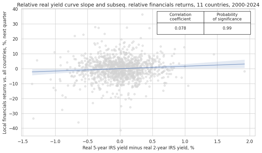
Steeper real yield curves predict country outperformance for finance stocks

Two of the main drivers for financial companies are net interest margin and credit generation. These can be proxied by JPMaQS quantamental indicators of real yields (difference between 2 and 5 years, using market implied inflation expectations) and the private credit growth in excess of nominal GDP growth.

These two have strong predictive power on the relative performance of financial equities across developed markets.

Specs and panel tests

using panel_calculator() method we create real yield slope RYLDSLOPE_NSA

cidx = cids_eqx

calcs = [
    "RYLDSLOPE_NSA = RYLDIRS05Y_NSA - RYLDIRS02Y_NSA",
    "PCREDIT_SJA_P1M1ML12vNGDP = PCREDITBN_SJA_P1M1ML12 - RGDP_SA_P1Q1QL4_20QMM - INFTEFF_NSA"
]

dfa = msp.panel_calculator(df=dfx, calcs=calcs, cids=cids_eqx)
dfx = msm.update_df(dfx, dfa)

Here we calculate the relative real yield curve slopes and give them postfix vGLB to indicate “versus Global Benchmark”

xcatx = ["RYLDSLOPE_NSA", "PCREDIT_SJA_P1M1ML12vNGDP"]

dfa = msp.make_relative_value(
    dfx,
    xcats=xcatx,
    cids=cidx,
    start="1990-01-01",
    rel_meth="subtract",
    postfix="vGLB",
)

dfx = msm.update_df(dfx, dfa)

cidx = cids_eqx
sigs = [
    "RYLDSLOPE_NSAvGLB",
    "PCREDIT_SJA_P1M1ML12vNGDP",
]
rets = ["EQCFINRUSD_NSAvGLB"]
start = "2000-01-01"

dict_fixc = {
    "sigs": sigs,
    "rets": rets,
    "cidx": cidx,
    "start": start,
    "black": None,
    "srr": None,
    "pnls": None,
}

CategoryRelations() function is used for quick visualization and analysis of two categories, in particular,

• Relative real yield curve slope RYLDSLOPE_NSAvGLB , and

• subseq. relative financials returns [ EQCFINRUSD_NSAvGLB ]

The .reg_scatter() method is convenient for visualizing the relationship between two categories, including the strength of the linear association and any potential outliers. It includes a regression line with a 95% confidence interval, which can help assess the significance of the relationship. The analysis is done on a quarterly basis.

dix = dict_fixc

sig = dix["sigs"][0]
ret = dix["rets"][0]
cidx = dix["cidx"]
blax = dix["black"]
start = dix["start"]

crx_mat = msp.CategoryRelations(
    dfx,
    xcats=[sig, ret],
    cids=cidx,
    freq="Q",
    lag=1,
    xcat_aggs=["last", "sum"],
    start=start,
    blacklist=None,
)
crx_mat.reg_scatter(
    labels=False,
    coef_box="upper right",
    xlab="Real 5-year IRS yield minus real 2-year IRS yield, %",
    ylab="Local financials returns vs. all countries, %, next quarter",
    title="Relative real yield curve slope and subseq. relative financials returns, 11 countries, 2000-2024",
    size=(10, 6),
    prob_est="map",
)

Accuracy and correlation check

SignalReturnRelations() function from the macrosynergy package analyses and compares the relationships between the chosen signals and the panel of subsequent returns. There is no regression analysis involved, rather the sign of the signal is used for predicting the sign of the target.

dix = dict_fixc

sigs = dix["sigs"]
rets = dix["rets"]
cidx = dix["cidx"]
blax = dix["black"]
start = dix["start"]

srr = mss.SignalReturnRelations(
    df=dfx,
    cids=cidx,
    sigs=sigs,
    rets=rets,
    freqs="M",
    start="1995-01-01",
)

mrt = srr.multiple_relations_table(rets=rets, xcats=sigs)

display(mrt.sort_index().astype("float").round(3)[xms])

				accuracy	bal_accuracy	pos_sigr	pos_retr	pearson	pearson_pval	kendall	kendall_pval
Return	Signal	Frequency	Aggregation
EQCFINRUSD_NSAvGLB	PCREDIT_SJA_P1M1ML12vNGDP	M	last	0.517	0.518	0.610	0.500	0.033	0.055	0.021	0.067
	RYLDSLOPE_NSAvGLB	M	last	0.514	0.514	0.516	0.501	0.054	0.002	0.024	0.037