Government bond volatility #
The category group contains data for bond benchmarks which span 9 countries and 7 tenors. This data comprises volatility and leverage ratios of vol-targeted positions in government bond benchmarks.
Generic government bond volatility #
Ticker : GB01YXRxEASD_NSA / GB02YXRxEASD_NSA / GB03YXRxEASD_NSA / GB05YXRxEASD_NSA / GB07YXRxEASD_NSA / GB10YXRxEASD_NSA / GB30YXRxEASD_NSA
Label : Government bond return volatility: 1-year maturity / 2-year maturity / 3-year maturity / 5-year maturity / 7-year maturity / 10-year maturity / 30-year maturity.
Definition : Annualised return standard deviation of government bond excess returns: 1-year maturity / 2-year maturity / 3-year maturity / 5-year maturity / 7-year maturity / 10-year maturity / 30-year maturity.
Notes :
-
The standard deviation has been calculated based on an exponential moving average of daily returns with a half-life of 11 active trading days.
-
The government yields used are spot rates taken from zero coupon curves that are available on J.P. Morgan DataQuery.
Leverage ratio of vol-targeted bond position #
Ticker : GB01YXRxLEV10_NSA / GB02YXRxLEV10_NSA / GB03YXRxLEV10_NSA / GB05YXRxLEV10_NSA / GB07YXRxLEV10_NSA / GB10YXRxLEV10_NSA / GB30YXRxLEV10_NSA
Label : Leverage ratio of bond position for 10% annualized vol target: 1-year maturity / 2-year maturity / 3-year maturity / 5-year maturity / 7-year maturity / 10-year maturity / 30-year maturity.
Definition : Bond leverage ratio for a 10% annualized vol target: 1-year maturity / 2-year maturity / 3-year maturity / 5-year maturity / 7-year maturity / 10-year maturity / 30-year maturity.
Notes :
-
This serves as the leverage ratio for a 10% annualized vol target and is inversely proportional to the estimated annualized standard deviation of the return on a government bond position.
-
A leverage ratio of 5 (for notional to risk capital) has been applied to simulate capital and risk management limits to leverage.
Generic government bond future volatility #
Ticker : GBF02YXRxEASD_NSA / GBF03YXRxEASD_NSA / GBF05YXRxEASD_NSA / GBF10YXRxEASD_NSA / GBF20YXRxEASD_NSA / GBF30YXRxEASD_NSA
Label : Government bond future return volatility: 2-year maturity / 3-year maturity / 5-year maturity / 10-year maturity / 20-year maturity / 30-year maturity.
Definition : Annualised return standard deviation of government bond future excess returns: 2-year maturity / 3-year maturity / 5-year maturity / 10-year maturity / 20-year maturity / 30-year maturity.
Notes :
-
The standard deviation has been calculated based on an exponential moving average of daily returns with a half-life of 11 active trading days.
-
The government bond future returns used are those computed by our continuous series of government bond future returns. See here for details on their calculation.
Imports #
Only the standard Python data science packages and the specialized
macrosynergy
package are needed.
import numpy as np
import pandas as pd
import matplotlib.pyplot as plt
import seaborn as sns
import math

import json
import yaml

import macrosynergy.management as msm
import macrosynergy.panel as msp
import macrosynergy.signal as mss
import macrosynergy.pnl as msn


from macrosynergy.download import JPMaQSDownload

from timeit import default_timer as timer
from datetime import timedelta, date, datetime
import os

import warnings

warnings.simplefilter("ignore")
The
JPMaQS
indicators we consider are downloaded using the J.P. Morgan Dataquery API interface within the
macrosynergy
package. This is done by specifying
ticker strings
, formed by appending an indicator category code
<category>
to a currency area code
<cross_section>
. These constitute the main part of a full quantamental indicator ticker, taking the form
DB(JPMAQS,<cross_section>_<category>,<info>)
, where
<info>
denotes the time series of information for the given cross-section and category. The following types of information are available:
-
valuegiving the latest available values for the indicator -
eop_lagreferring to days elapsed since the end of the observation period -
mop_lagreferring to the number of days elapsed since the mean observation period -
gradedenoting a grade of the observation, giving a metric of real time information quality.
After instantiating the
JPMaQSDownload
class within the
macrosynergy.download
module, one can use the
download(tickers,start_date,metrics)
method to easily download the necessary data, where
tickers
is an array of ticker strings,
start_date
is the first collection date to be considered and
metrics
is an array comprising the times series information to be downloaded.
cids = ["AUD", "DEM", "FRF", "ESP", "ITL", "JPY", "NZD", "GBP", "USD", "CNY"]
vols = [
    "GB01YXRxEASD_NSA",
    "GB02YXRxEASD_NSA",
    "GB03YXRxEASD_NSA",
    "GB05YXRxEASD_NSA",
    "GB07YXRxEASD_NSA",
    "GB10YXRxEASD_NSA",
    "GB30YXRxEASD_NSA",
]
carry = [
    "GB01YCRY_VT10",
    "GB02YCRY_VT10",
    "GB03YCRY_VT10",
    "GB05YCRY_VT10",
    "GB07YCRY_VT10",
    "GB30YCRY_VT10",
    "GB01YCRY_NSA",
    "GB02YCRY_NSA",
    "GB03YCRY_NSA",
    "GB05YCRY_NSA",
    "GB07YCRY_NSA",
    "GB10YCRY_NSA",
    "GB30YCRY_NSA",
]
levs = [
    "GB01YXRxLEV10_NSA",
    "GB02YXRxLEV10_NSA",
    "GB03YXRxLEV10_NSA",
    "GB05YXRxLEV10_NSA",
    "GB07YXRxLEV10_NSA",
    "GB10YXRxLEV10_NSA",
    "GB30YXRxLEV10_NSA",
]
futs = [
    "GBF02YXRxEASD_NSA",
    "GBF03YXRxEASD_NSA",
    "GBF05YXRxEASD_NSA",
    "GBF10YXRxEASD_NSA",
    "GBF20YXRxEASD_NSA",
    "GBF30YXRxEASD_NSA",
]

xcats = vols + carry + levs + futs
# Download series from J.P. Morgan DataQuery by tickers

start_date = "1990-01-01"
tickers = [cid + "_" + xcat for cid in cids for xcat in xcats]
print(f"Maximum number of tickers is {len(tickers)}")

# Retrieve credentials

client_id: str = os.getenv("DQ_CLIENT_ID")
client_secret: str = os.getenv("DQ_CLIENT_SECRET")

# Download from DataQuery

with JPMaQSDownload(client_id=client_id, client_secret=client_secret) as downloader:
    start = timer()
    assert downloader.check_connection()
    df = downloader.download(
        tickers=tickers,
        start_date=start_date,
        metrics=["value", "eop_lag", "mop_lag", "grading"],
        suppress_warning=True,
    )
    end = timer()

dfd = df

print("Download time from DQ: " + str(timedelta(seconds=end - start)))
Maximum number of tickers is 330
Downloading data from JPMaQS.
Timestamp UTC:  2025-02-28 09:17:59
Connection successful!
Some expressions are missing from the downloaded data. Check logger output for complete list.
248 out of 1320 expressions are missing. To download the catalogue of all available expressions and filter the unavailable expressions, set `get_catalogue=True` in the call to `JPMaQSDownload.download()`.
Some dates are missing from the downloaded data.
265 out of 9177 dates are missing.
Download time from DQ: 0:01:15.662104
Availability #
cids_exp = cids  # cids expected in category panels
msm.missing_in_df(dfd, xcats=xcats, cids=cids_exp)
No missing XCATs across DataFrame.
Missing cids for GB01YCRY_NSA:       ['CNY']
Missing cids for GB01YCRY_VT10:      ['CNY']
Missing cids for GB01YXRxEASD_NSA:   ['CNY']
Missing cids for GB01YXRxLEV10_NSA:  ['CNY']
Missing cids for GB02YCRY_NSA:       ['CNY']
Missing cids for GB02YCRY_VT10:      ['CNY']
Missing cids for GB02YXRxEASD_NSA:   ['CNY']
Missing cids for GB02YXRxLEV10_NSA:  ['CNY']
Missing cids for GB03YCRY_NSA:       ['CNY']
Missing cids for GB03YCRY_VT10:      ['CNY']
Missing cids for GB03YXRxEASD_NSA:   ['CNY']
Missing cids for GB03YXRxLEV10_NSA:  ['CNY']
Missing cids for GB05YCRY_NSA:       ['CNY']
Missing cids for GB05YCRY_VT10:      ['CNY']
Missing cids for GB05YXRxEASD_NSA:   ['CNY']
Missing cids for GB05YXRxLEV10_NSA:  ['CNY']
Missing cids for GB07YCRY_NSA:       ['CNY']
Missing cids for GB07YCRY_VT10:      ['CNY']
Missing cids for GB07YXRxEASD_NSA:   ['CNY']
Missing cids for GB07YXRxLEV10_NSA:  ['CNY']
Missing cids for GB10YCRY_NSA:       ['CNY']
Missing cids for GB10YXRxEASD_NSA:   ['CNY']
Missing cids for GB10YXRxLEV10_NSA:  ['CNY']
Missing cids for GB30YCRY_NSA:       ['CNY']
Missing cids for GB30YCRY_VT10:      ['CNY']
Missing cids for GB30YXRxEASD_NSA:   ['CNY']
Missing cids for GB30YXRxLEV10_NSA:  ['CNY']
Missing cids for GBF02YXRxEASD_NSA:  ['AUD', 'ESP', 'FRF', 'JPY', 'NZD']
Missing cids for GBF03YXRxEASD_NSA:  ['CNY', 'DEM', 'ESP', 'FRF', 'GBP', 'ITL', 'JPY', 'NZD', 'USD']
Missing cids for GBF05YXRxEASD_NSA:  ['ESP', 'FRF', 'ITL', 'JPY', 'NZD']
Missing cids for GBF10YXRxEASD_NSA:  ['NZD']
Missing cids for GBF20YXRxEASD_NSA:  ['CNY', 'DEM', 'ESP', 'FRF', 'GBP', 'ITL', 'NZD', 'USD']
Missing cids for GBF30YXRxEASD_NSA:  ['AUD', 'CNY', 'ESP', 'FRF', 'ITL', 'JPY', 'NZD']
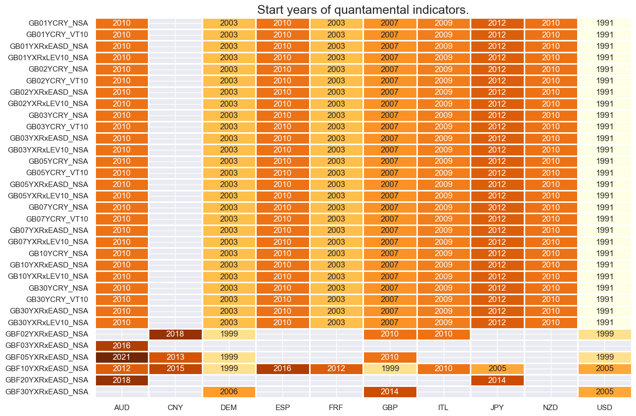
U.S. data are available from the early 1990s but series of other bonds markets only start from post-2000.
xcatx = xcats
cidx = cids_exp

dfx = msm.reduce_df(dfd, xcats=xcatx, cids=cidx)
dfs = msm.check_startyears(
    dfx,
)
msm.visual_paneldates(dfs, size=(14, 10))

print("Last updated:", date.today())
Last updated: 2025-02-28
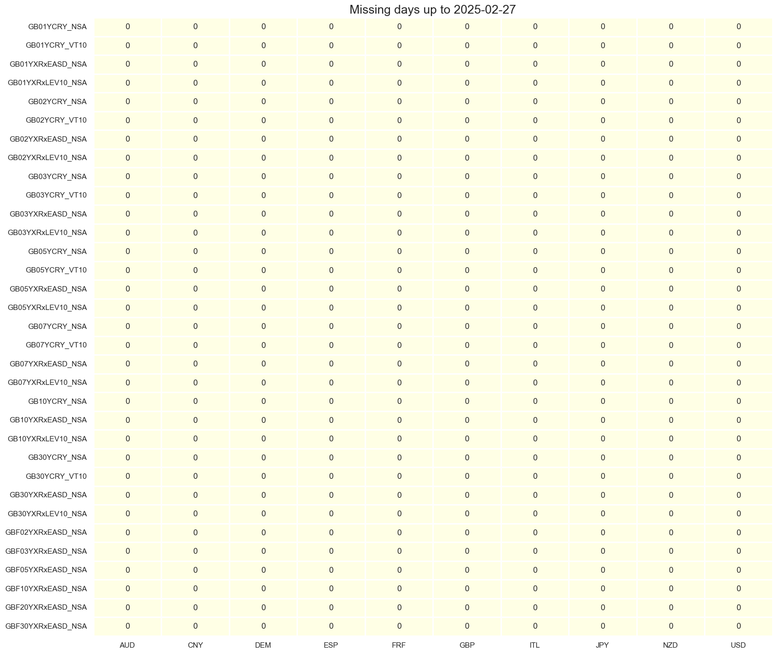
xcatx = xcats
cidx = cids_exp

plot = msm.check_availability(
    dfd, xcats=xcatx, cids=cids_exp, start_size=(18, 6), start_years=False
)
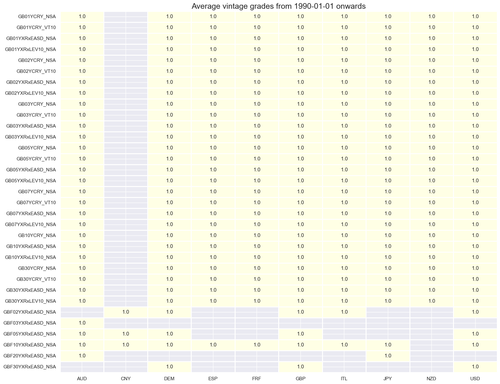
xcatx = xcats
cidx = cids_exp

plot = msp.heatmap_grades(
    dfd,
    xcats=xcatx,
    cids=cidx,
    size=(18, 15),
    title=f"Average vintage grades from {start_date} onwards",
)
xcats_bond_vol = ["GB01YXRxEASD_NSA", "GB02YXRxEASD_NSA"]

msp.view_ranges(
    dfd,
    xcats=xcats_bond_vol,
    cids=cids,
    val="eop_lag",
    title="End of observation period lags (ranges of time elapsed since end of observation period in days), government bond volatility",
    start="2000-01-01",
    kind="box",
    size=(16, 4),
)

msp.view_ranges(
    dfd,
    xcats=xcats_bond_vol,
    cids=cids,
    val="mop_lag",
    title="Median of observation period lags (ranges of time elapsed since middle of observation period in days), government bond volatility",
    start="2000-01-01",
    kind="box",
    size=(16, 4),
)

xcats_lev = ["GB01YXRxLEV10_NSA", "GB02YXRxLEV10_NSA"]

msp.view_ranges(
    dfd,
    xcats=xcats_lev,
    cids=cids,
    val="eop_lag",
    title="End of observation period lags (ranges of time elapsed since end of observation period in days), leverage ratio of vol-targeted bond position",
    start="2000-01-01",
    kind="box",
    size=(16, 4),
)

msp.view_ranges(
    dfd,
    xcats=xcats_lev,
    cids=cids,
    val="mop_lag",
    title="Median of observation period lags (ranges of time elapsed since middle of observation period in days), leverage ratio of vol-targeted bond position",
    start="2000-01-01",
    kind="box",
    size=(16, 4),
)
xcats_future = ["GBF02YXRxEASD_NSA", "GBF03YXRxEASD_NSA"]

msp.view_ranges(
    dfd,
    xcats=xcats_future,
    cids=cids,
    val="eop_lag",
    title="End of observation period lags (ranges of time elapsed since end of observation period in days), government bond future volatility",
    start="2000-01-01",
    kind="box",
    size=(16, 4),
)

msp.view_ranges(
    dfd,
    xcats=xcats_future,
    cids=cids,
    val="mop_lag",
    title="Median of observation period lags (ranges of time elapsed since middle of observation period in days), government bond future volatility",
    start="2000-01-01",
    kind="box",
    size=(16, 4),
)

History #
Government bond volatility #
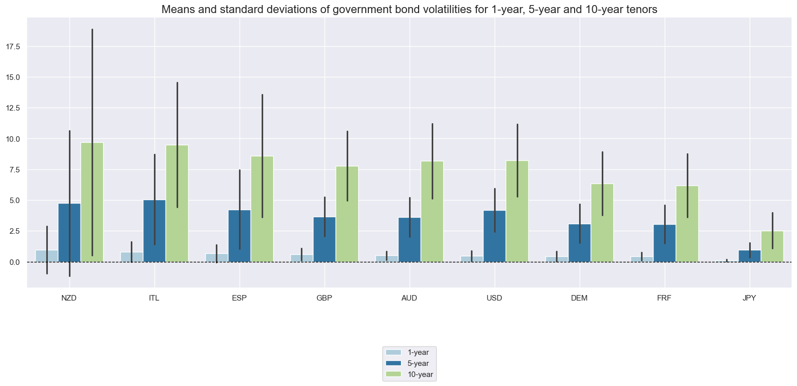
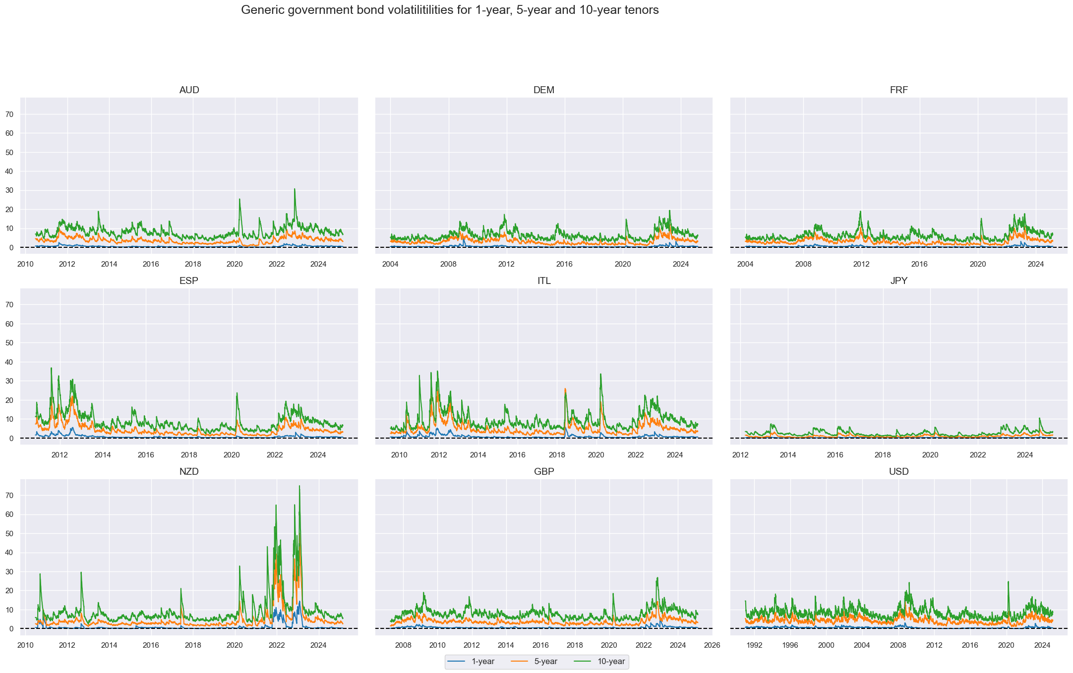
Return volatility increases with maturity across all available countries. Japan’s volatility level and ranges have been compressed over the sample period.
xcatx = ["GB01YXRxEASD_NSA", "GB05YXRxEASD_NSA", "GB10YXRxEASD_NSA"]
cidx = cids_exp

msp.view_ranges(
    dfd,
    xcats=xcatx,
    cids=cidx,
    sort_cids_by="mean",
    start="2000-01-01",
    title="Means and standard deviations of government bond volatilities for 1-year, 5-year and 10-year tenors",
    xcat_labels=["1-year", "5-year", "10-year"],
    kind="bar",
    size=(16, 8),
)
Government bond volatility has been higher in periods of financial stress, for instance during the 2008 crisis, during the european debt crisis in 2011 and especially at the beginning of the COVID-19 pandemic.
xcatx = ["GB01YXRxEASD_NSA", "GB05YXRxEASD_NSA", "GB10YXRxEASD_NSA"]
cidx = cids

msp.view_timelines(
    dfd,
    xcats=xcatx,
    cids=cidx,
    start="1990-01-01",
    title="Generic government bond volatilitilities for 1-year, 5-year and 10-year tenors",
    title_adj=1.05,
    title_xadj=0.42,
    xcat_labels=["1-year", "5-year", "10-year"],
    label_adj=0.1,
    ncol=3,
    same_y=True,
    size=(12, 7),
    aspect=1.7,
    all_xticks=True,
)
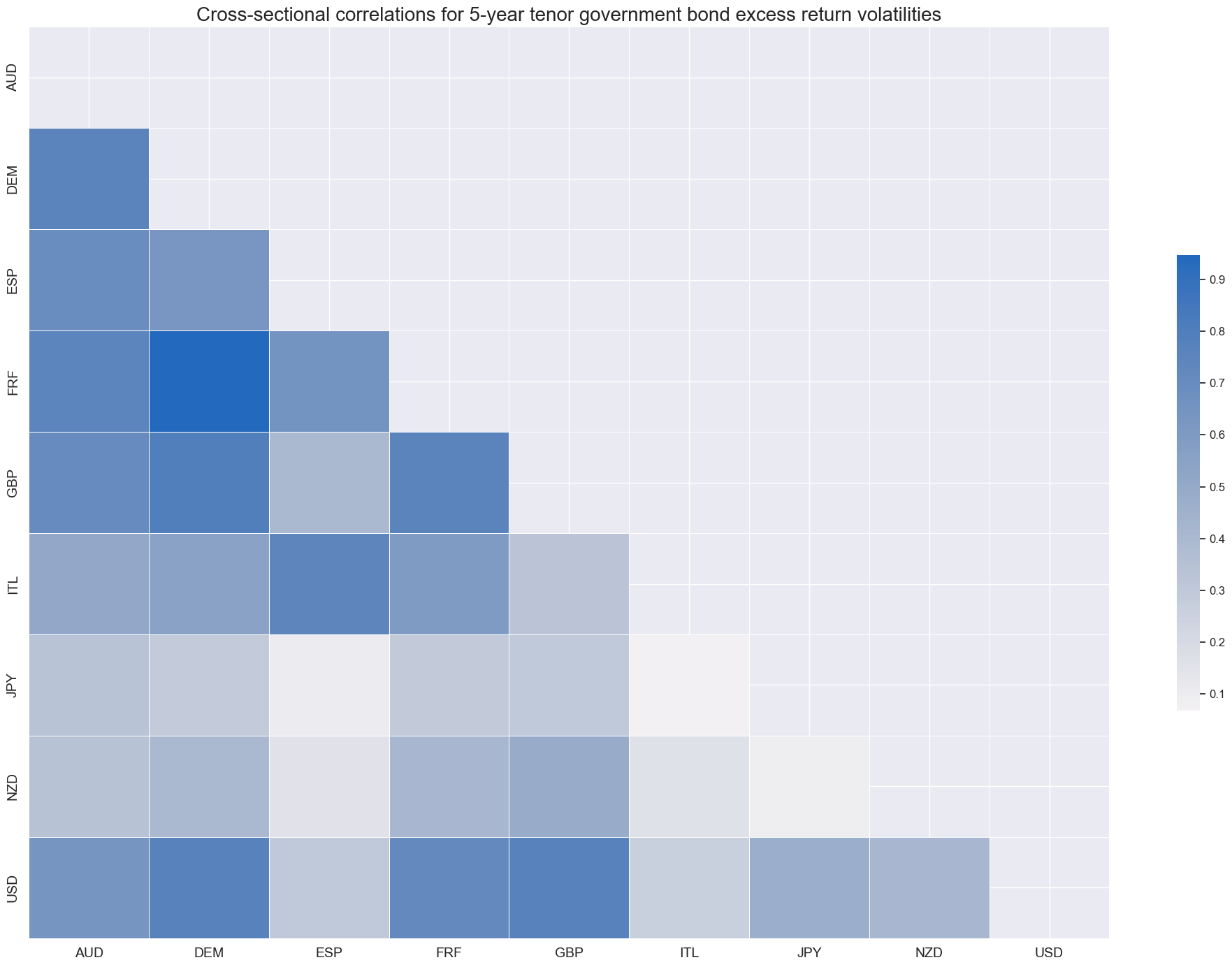
Government bond return volatility has been highly positively correlated across countries.
xcatx = "GB05YXRxEASD_NSA"
cidx = cids

msp.correl_matrix(
    dfd,
    xcats=xcatx,
    cids=cidx,
    title="Cross-sectional correlations for 5-year tenor government bond excess return volatilities",
    size=(20, 14),
)
Leverage ratio #
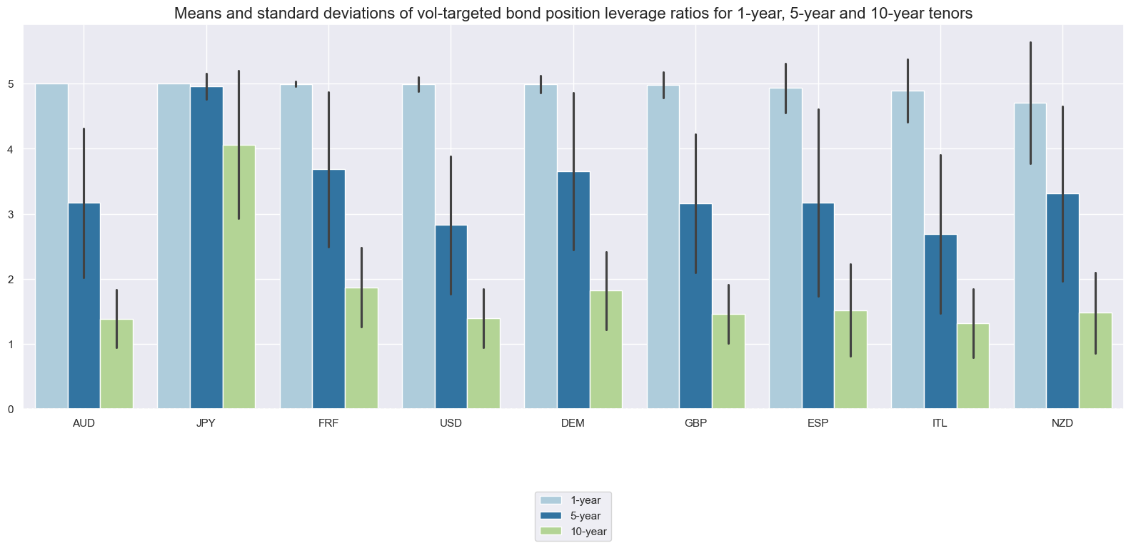
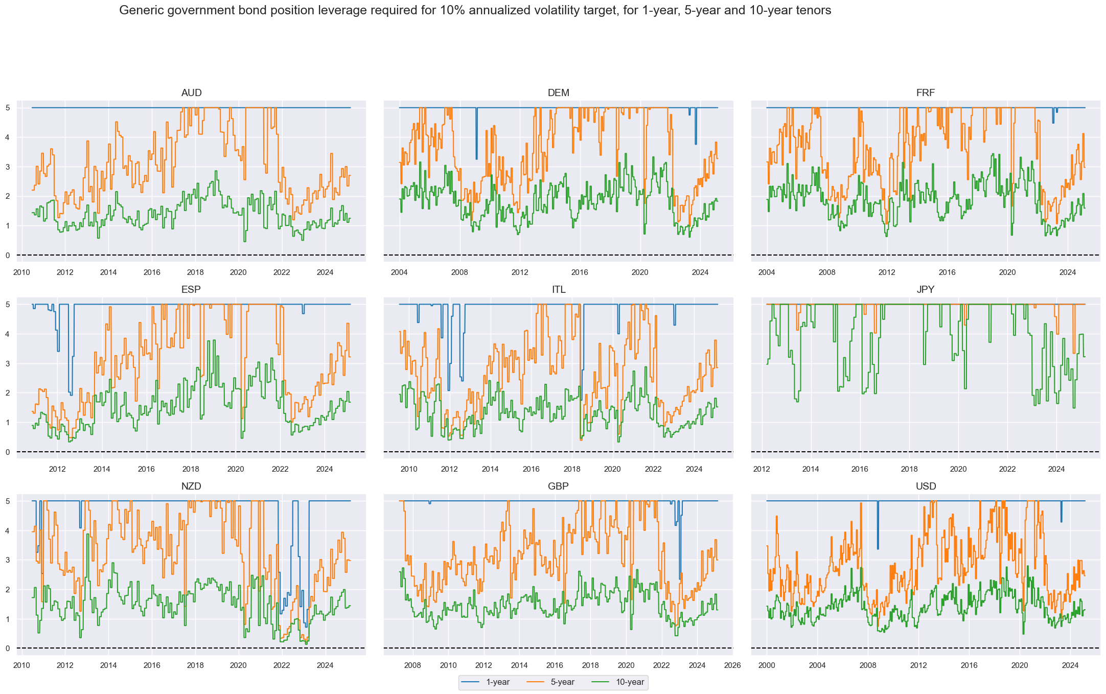
Required leverage ratios for 10% volatility targets averaged between 1.5 and 5 across currency areas. Due to short yield compression near the zero boundary, a 10% volatility target would mostly have required more leverage than allowed by our standard parameters.
xcatx = ["GB01YXRxLEV10_NSA", "GB05YXRxLEV10_NSA", "GB10YXRxLEV10_NSA"]
cidx = cids

msp.view_ranges(
    dfd,
    xcats=xcatx,
    cids=cidx,
    sort_cids_by="mean",
    start="2000-01-01",
    kind="bar",
    title="Means and standard deviations of vol-targeted bond position leverage ratios for 1-year, 5-year and 10-year tenors",
    xcat_labels=["1-year", "5-year", "10-year"],
    size=(16, 8),
)
xcatx = ["GB01YXRxLEV10_NSA", "GB05YXRxLEV10_NSA", "GB10YXRxLEV10_NSA"]
cidx = cids

msp.view_timelines(
    dfd,
    xcats=xcatx,
    cids=cidx,
    start="2000-01-01",
    title_adj=1.05,
    title_xadj=0.43,
    title="Generic government bond position leverage required for 10% annualized volatility target, for 1-year, 5-year and 10-year tenors",
    xcat_labels=["1-year", "5-year", "10-year"],
    label_adj=0.1,
    cumsum=False,
    ncol=3,
    same_y=True,
    size=(12, 7),
    aspect=1.7,
    all_xticks=True,
)
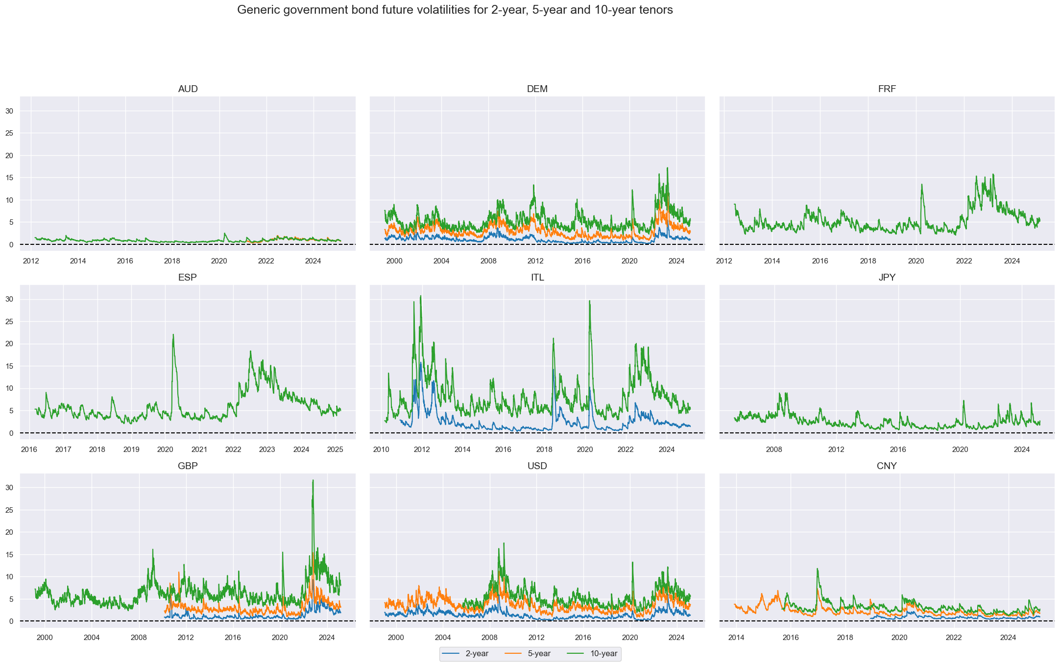
Government bond future volatility #
Bond future volatility seems to average 5% in most cases, increasing in periods of market stress – such as during the global financial crisis and right after the COVID-19 pandemic outbreak. Volatility has remained compressed during the period of ample purchases by central banks, from the year 2011 to the year 2018.
xcatx = ["GBF02YXRxEASD_NSA", "GBF05YXRxEASD_NSA", "GBF10YXRxEASD_NSA"]
cidx = cids

msp.view_timelines(
    dfd,
    xcats=xcatx,
    cids=cidx,
    start="1990-01-01",
    title="Generic government bond future volatilities for 2-year, 5-year and 10-year tenors",
    title_adj=1.05,
    title_xadj=0.43,
    xcat_labels=["2-year", "5-year", "10-year"],
    label_adj=0.1,
    ncol=3,
    same_y=True,
    size=(12, 7),
    aspect=1.7,
    all_xticks=True,
)
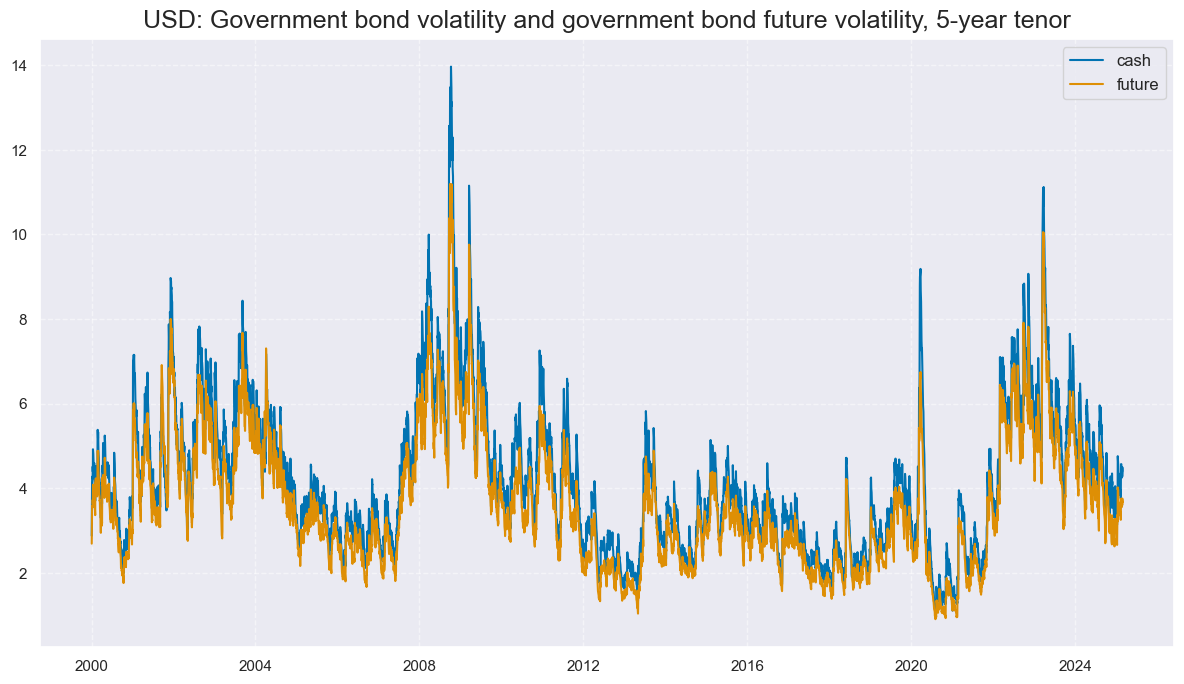
In the United States, bond future volatility has been consistently lower than the volatility of the cash product. This makes sense because the bond future is more liquid than the cash, therefore will see its volatility being compressed.
xcatx = ["GB05YXRxEASD_NSA", "GBF05YXRxEASD_NSA"]
cidx = ["USD"]
msp.view_timelines(
    dfd,
    xcats=xcatx,
    cids=cidx,
    start="2000-01-01",
    title="USD: Government bond volatility and government bond future volatility, 5-year tenor",
    xcat_labels=["cash", "future"],
    ncol=1,
    same_y=False,
    size=(12, 7),
    aspect=1.7,
)
Importance #
Research links #
“Even though government bonds are safe assets, large holdings by leveraged investors may detract from orderly market functioning and may necessitate interventions by the central bank.” Schrimpf, Shin, and Sushko
“As before, we asked the question, ‘Did they bet the ranch?’ For those hedge funds that had positions in European bonds, their total bet size was roughly two times their capital base. This is not an excessive leverage by normal hedge fund standards”. Fung et al
Empirical clues #
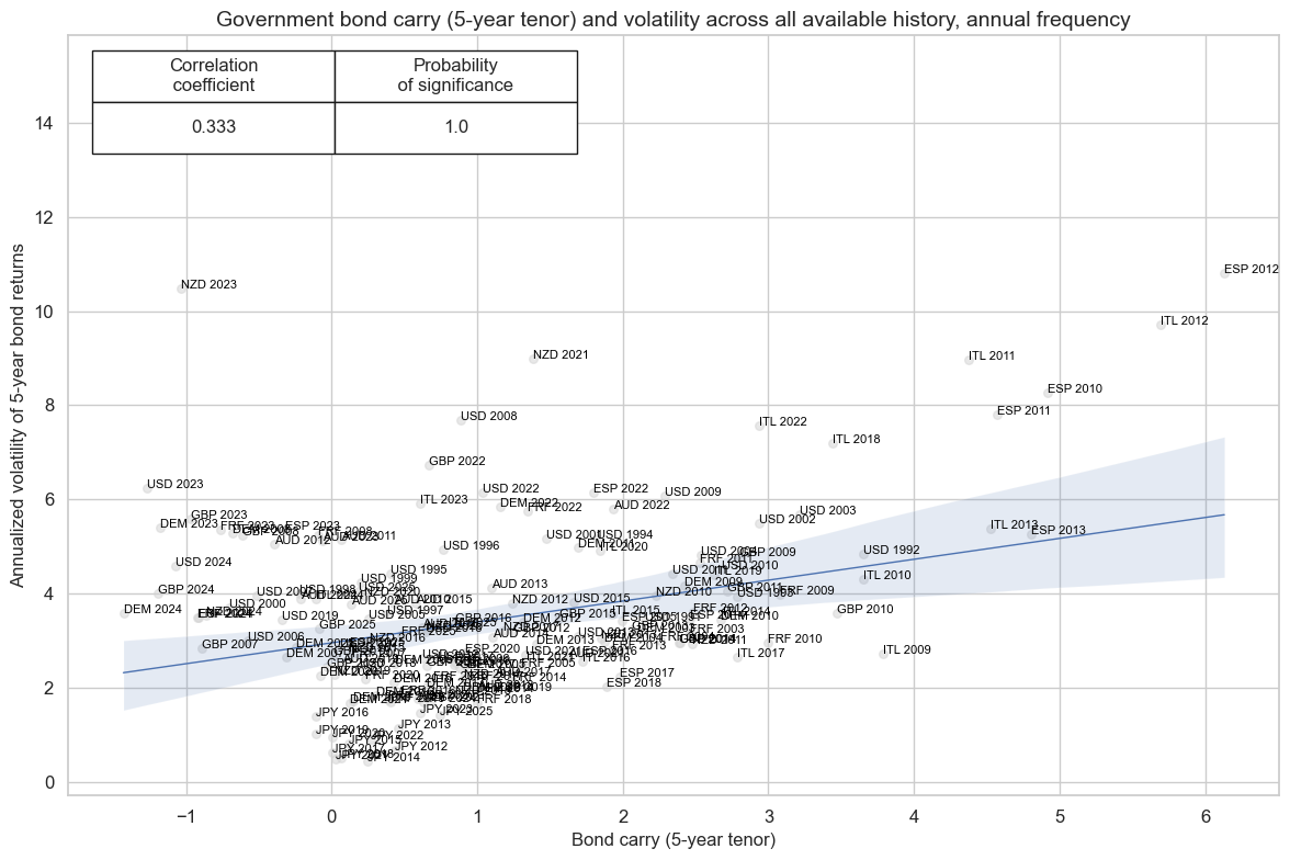
There has been a strong positive correlation between bond carry and return volatility across the panel.
xcatx = ["GB05YCRY_NSA", "GB05YXRxEASD_NSA"]
cidx = cids

cr = msp.CategoryRelations(
    dfd,
    xcats=xcatx,
    cids=cidx,
    freq="A",
    lag=0,
    xcat_aggs=["mean", "mean"],
    start="1990-01-01",
    years=None,
)

cr.reg_scatter(
    title="Government bond carry (5-year tenor) and volatility across all available history, annual frequency",
    labels=True,
    reg_robust=True,
    coef_box="upper left",
    xlab="Bond carry (5-year tenor)",
    ylab="Annualized volatility of 5-year bond returns",
)
GB05YCRY_NSA misses: ['CNY'].
GB05YXRxEASD_NSA misses: ['CNY'].
Appendices #
Appendix 1: Currency symbols #
The word ‘cross-section’ refers to currencies, currency areas or economic areas. In alphabetical order, these are AUD (Australian dollar), BRL (Brazilian real), CAD (Canadian dollar), CHF (Swiss franc), CLP (Chilean peso), CNY (Chinese yuan renminbi), COP (Colombian peso), CZK (Czech Republic koruna), DEM (German mark), ESP (Spanish peseta), EUR (Euro), FRF (French franc), GBP (British pound), HKD (Hong Kong dollar), HUF (Hungarian forint), IDR (Indonesian rupiah), ITL (Italian lira), JPY (Japanese yen), KRW (Korean won), MXN (Mexican peso), MYR (Malaysian ringgit), NLG (Dutch guilder), NOK (Norwegian krone), NZD (New Zealand dollar), PEN (Peruvian sol), PHP (Phillipine peso), PLN (Polish zloty), RON (Romanian leu), RUB (Russian ruble), SEK (Swedish krona), SGD (Singaporean dollar), THB (Thai baht), TRY (Turkish lira), TWD (Taiwanese dollar), USD (U.S. dollar), ZAR (South African rand).