General government finance ratios

This category group contains public finance ratios according to IMF methodology. The focus is on semi-official (IMF) point-in-time early estimates of various types of balances as well as revenue and expenditure ratios to concurrent GDP.

These indicators are indicative of government default risk, governments’ scope for intervening in the economy and the public sector influence on private sector activity, and hence give an investor valuable information on how different governments behave in different periods of health of an economy. As with most indicators in the macroeconomic balance sheets theme, the general government finance ratios are indicative of underlying risks to financial stability that could escalate when funding conditions deteriorate.

General government balance ratios

Ticker : GGOBGDPRATIO_NSA / GGPBGDPRATIO_NSA / GGSBGDPRATIO_NSA / GGOBGDPRATIONY_NSA / GGPBGDPRATIONY_NSA / GGSBGDPRATIONY_NSA / GGOBGDPRATIOPY_NSA / GGPBGDPRATIOPY_NSA / GGSBGDPRATIOPY_NSA

Label : General government balance, % of GDP: overall current year / primary current year / structural current year / overall next year / primary next year / structural next year / overall previous year / primary previous year / structural previous year

Definition : General government balance, IMF estimate, as % of GDP: overall current year / primary current year / structural current year / overall next year / primary next year / structural next year / overall previous year / primary previous year / structural previous year

Notes :

• General government is defined as the total of central, state and local governments including the social security funds controlled by these units.

• For observation period ‘current year’: the values are estimates, typically based on the budget law and the IMF staff economic analysis. For instance, for a December 30, 2022 real-time date, the observation period would 2022. For a January 2, 2023 real-time date the observation period would be 2023. Moreover, the IMF typically updates annual estimates in early spring and autumn.

• For ‘next year’, this is the next year estimate of the fiscal monitor ratios as published by the IMF in their biannual fiscal monitor publication. In this instance, the observation period is always the next year. The values are estimates, typically based on the budget law and the IMF staff economic analysis. For instance, for a December 30, 2022 real-time date, the observation period would 2023. For a January 2, 2023 real-time date the observation period would be 2024.

• For ‘previous year’, this is the previous year estimate of the fiscal monitor ratios as published by the IMF in their biannual fiscal monitor publication. In this instance, the observation period is always the previous year. The values are estimates, typically based on the budget law and the IMF staff economic analysis. For instance, for a December 30, 2022 real-time date, the observation period would 2021. For a January 2, 2023 real-time date the observation period would be 2022.

• The overall balance is defined as the difference between overall government revenues and expenditures. Expenditures include interest spending, i.e. they are affected by debt servicing costs.

• The primary balance is defined as the difference between overall government revenues and non-interest expenditures. Conceptually it is “the difference between the amount of revenue a government collects and the amount it spends on providing public goods and services” (OECD).

• The structural balance is defined as the difference between overall government revenues and expenditures, adjusted by the estimated effect of a broad set of transitory factors such as commodity shocks, housing, stock, and other asset price cycles, output composition and absorption effects and one-off factors. The adjustment is based on estimates by IMF staff.

• Primary balances for China only have vintages going back to 2015.

• There is no primary balance data for Taiwan.

• Singapore’s primary balance estimates have not been released in The October 2017 and October 2019 reviews and have not been updated since October 2021.

• Primary balances for the US miss some observation dates for release dates 2011-2013.

• Structural balances for Thailand are missing the April 2020 data point.

• For Venezuela, the IMF states that assessing past and current economic developments has been compromised by the lack of discussions with authorities. For the year 2020 and 2021, the IMF did not publish projections for any fiscal balances. JPMaQS applied last available figures for these years, resulting in long publication lags. Also, there is generally no net debt data available for Venezuela.

• There are no structural government balance data available for Nigeria, Oman, Qatar, Serbia and the UAE.

• See also source data notes in Appendix 1 .

General government revenue ratio

Ticker : GGRGDPRATIO_NSA / GGRGDPRATIONY_NSA / GGRGDPRATIOPY_NSA

Label : General government revenues, % of GDP: current year / next year / previous year

Definition : Estimated general government revenues, as % of GDP: current year / next year / previous year

Notes :

• General government is defined as the total of central, state and local governments including the social security funds controlled by these units.

• The observation period is always the current year. The values are estimates, typically based on the budget law and the IMF staff economic analysis.

• Revenues include taxes, typically as the largest item. In addition, Other revenues include property income derived from the ownership of assets, sales of goods and services, and voluntary transfers received from other units.

• Taiwan has no vintage data prior to 2011.

• Likewise, in Spain vintages before 2010 have too many missing values to be used.

• See also source data notes in Appendix 1 .

General government expenditure ratio

Ticker : GGEGDPRATIO_NSA / GGEGDPRATIONY_NSA / GGEGDPRATIOPY_NSA

Label : General government expenditures, % of GDP: current year / next year / previous year

Definition : Estimated general government expenditures, as % of GDP: current year / next year / previous year

Notes :

• General government is defined as the total of central, state and local governments including the social security funds controlled by these units.

• The observation period is always the current year. The values are estimates, typically based on the budget law and the IMF staff economic analysis.

• Expenditures are defined as the expenses incurred by government for the delivery of public goods, services, and social protection.

• For Taiwan, we did not add the 2020 vintage as there are too many missing observation dates.

• For the US, the IMF has not stored values for pre-2000 observation dates for release dates from 2002 to 2012.

• See also source data notes in Appendix 1 .

General government debt ratios

Ticker : GGDGDPRATIO_NSA / GGNDGDPRATIO_NSA / GGDGDPRATIONY_NSA / GGNDGDPRATIONY_NSA / GGDGDPRATIOPY_NSA / GGNDGDPRATIOPY_NSA

Label : General government debt, % of GDP: gross current year / net current year / gross next year / net next year / gross previous year / net previous year

Definition : General government debt, IMF estimate, as % of GDP: gross current year / net current year / gross next year / net next year / gross previous year / net previous year

Notes :

• General government is defined as the total of central, state and local governments including the social security funds controlled by these units.

• The observation period is always the current year. The values are estimates, typically based on the budget law and the IMF staff economic analysis.

• Gross government debt is defined as the total of liabilities that require payment of interest and/or principal at any time in the future. This includes debt securities, loans, insurances, special drawing rights, deposits, pensions and standardized guarantee schemes.

• Net government debt is calculated as gross debt minus financial assets.

• For each release date, the observation period of the value is the concurrent year’s estimate, which is based on the budget and the IMF’s economic analysis. For instance, for the October 2022 release, the observation period will be 2022.

• Net debt calculations for Norway were revised by the IMF starting with the October 2017 publication, excluding the equity and shares from financial assets and including accounts receivable in the financial assets, following Government Finance Statistics and the Maastricht definition.

• Net debt data are not available for China, India, Russia, Singapore and Thailand.

• Norway’s net debt series shows a large revision in 2022 operated by the IMF and following a change in the net debt calculation, ‘which excludes the eqity and shares from financial assets and includes accounts receivable in the financial assets, following the Government Finance Statistics Manual 2014 and the Maastricht definition’.

• See also source data notes in Appendix 1 .

General government fiscal thrust

Ticker : GGFTGDPRATIO_NSA / GGFTGDPRATIONY_NSA / GGFTGDPRATIOPY_NSA

Label : Fiscal thrust, % of GDP: current year / next year / previous year

Definition : General government fiscal thrust, observation year versus previous, IMF estimate, as % of GDP: current year of observation / previous year of observation / next year of observation

Notes :

• Fiscal thrust, also called fiscal impulse, measures the direct impact of fiscal policy on aggregate demand in the economy.

• It is approximated by the negative of the difference between a country’s (expected or estimated) structural balance as % of GDP in the current years versus the previous year.

• Since structural balances are adjusted for the impact of business cycles and terms-of-trade they are indicative of the stance of fiscal policy, i.e. the effect of discretionary fiscal measures on the economy. A positive value means that the structural balance shifts towards deficit and that policy is expansionary. A negative value means that the structural balance has shifts towards surplus and that policy is restrictive.

• General government is defined as the total of central, state and local governments including the social security funds controlled by these units.

• The observation period is always the current year. The values are estimates, typically based on the budget law and the IMF staff economic analysis.

• See also source data notes in Appendix 1 .

Imports

Only the standard Python data science packages and the specialized macrosynergy package are needed.

import os
import pandas as pd

import macrosynergy.management as msm
import macrosynergy.panel as msp
import macrosynergy.visuals as msv
from macrosynergy.download import JPMaQSDownload

from timeit import default_timer as timer
from datetime import timedelta, date

import warnings

warnings.simplefilter("ignore")

/Library/Frameworks/Python.framework/Versions/3.11/lib/python3.11/site-packages/tqdm/auto.py:21: TqdmWarning: IProgress not found. Please update jupyter and ipywidgets. See https://ipywidgets.readthedocs.io/en/stable/user_install.html
  from .autonotebook import tqdm as notebook_tqdm

The JPMaQS indicators we consider are downloaded using the J.P. Morgan Dataquery API interface within the macrosynergy package. This is done by specifying ticker strings , formed by appending an indicator category code <category> to a currency area code <cross_section> . These constitute the main part of a full quantamental indicator ticker, taking the form DB(JPMAQS,<cross_section>_<category>,<info>) , where <info> denotes the time series of information for the given cross-section and category. The following types of information are available:

• value giving the latest available values for the indicator

• eop_lag referring to days elapsed since the end of the observation period

• mop_lag referring to the number of days elapsed since the mean observation period

• grade denoting a grade of the observation, giving a metric of real time information quality.

After instantiating the JPMaQSDownload class within the macrosynergy.download module, one can use the download(tickers,start_date,metrics) method to easily download the necessary data, where tickers is an array of ticker strings, start_date is the first collection date to be considered and metrics is an array comprising the times series information to be downloaded.

# Cross-sections of interest

cids_dmca = [
    "AUD",
    "CAD",
    "CHF",
    "EUR",
    "GBP",
    "JPY",
    "NOK",
    "SEK",
    "USD",
]  # DM currency areas
cids_dmec = ["DEM", "ESP", "FRF", "ITL"]  # DM euro area countries
cids_latm = ["COP", "CLP", "MXN", "PEN"]  # Latam countries
cids_emea = ["ILS", "PLN", "RON", "RUB", "ZAR"]  # EMEA countries
cids_emas = [
    "CNY",
    "IDR",
    "INR",
    "KRW",
    "SGD",
    "THB",
    "TWD",
    "NZD",
]  # EM Asia countries

cids_frontier = ['AED', 'ARS', 'DOP', 'EGP', 'NGN', 'OMR', 'PAB', 'QAR', 'RSD', 'SAR', 'UYU', 'VEF']

cids_dm = cids_dmca + cids_dmec
cids_em = cids_latm + cids_emea + cids_emas

cids = sorted(cids_dm + cids_em + cids_frontier)

# Quantamental categories of interest

main = [
    "GGOBGDPRATIO_NSA",
    "GGPBGDPRATIO_NSA",
    "GGSBGDPRATIO_NSA",
    "GGRGDPRATIO_NSA",
    "GGEGDPRATIO_NSA",
    "GGFTGDPRATIO_NSA",
    "GGDGDPRATIO_NSA",
    "GGNDGDPRATIO_NSA",
]
special = [
    "GGOBGDPRATIONY_NSA",
    "GGPBGDPRATIONY_NSA",
    "GGSBGDPRATIONY_NSA",
    "GGRGDPRATIONY_NSA",
    "GGEGDPRATIONY_NSA",
    "GGFTGDPRATIONY_NSA",
    "GGDGDPRATIONY_NSA",
    "GGNDGDPRATIONY_NSA",
    "GGOBGDPRATIOPY_NSA",
    "GGPBGDPRATIOPY_NSA",
    "GGSBGDPRATIOPY_NSA",
    "GGRGDPRATIOPY_NSA",
    "GGEGDPRATIOPY_NSA",
    "GGFTGDPRATIOPY_NSA",
    "GGDGDPRATIOPY_NSA",
    "GGNDGDPRATIOPY_NSA",
]
econ = []
mark = ["DU05YXR_NSA", 
        "DU05YXR_VT10",
        "FCBIR_NSA",
        "FXTARGETED_NSA", "FXUNTRADABLE_NSA"
       ]  # market links

xcats = main + econ + mark + special

# Download series from J.P. Morgan DataQuery by tickers

start_date = "1990-01-01"
tickers = [cid + "_" + xcat for cid in cids for xcat in xcats]
print(f"Maximum number of tickers is {len(tickers)}")

# Retrieve credentials

client_id: str = os.getenv("DQ_CLIENT_ID")
client_secret: str = os.getenv("DQ_CLIENT_SECRET")

# Download from DataQuery

with JPMaQSDownload(client_id=client_id, client_secret=client_secret) as downloader:
    start = timer()
    df = downloader.download(
        tickers=tickers,
        start_date=start_date,
        metrics=["value", "eop_lag", "mop_lag", "grading"],
        suppress_warning=True,
        show_progress=True,
    )
    end = timer()


print("Download time from DQ: " + str(timedelta(seconds=end - start)))

Maximum number of tickers is 1218
Downloading data from JPMaQS.
Timestamp UTC:  2025-02-27 15:08:53
Connection successful!

Requesting data: 100%|████████████████████████| 244/244 [00:53<00:00,  4.60it/s]
Downloading data: 100%|███████████████████████| 244/244 [04:00<00:00,  1.01it/s]

Some expressions are missing from the downloaded data. Check logger output for complete list.
668 out of 4872 expressions are missing. To download the catalogue of all available expressions and filter the unavailable expressions, set `get_catalogue=True` in the call to `JPMaQSDownload.download()`.
Download time from DQ: 0:05:18.447527

Availability

cids_exp = cids  # cids expected in category panels
msm.missing_in_df(df, xcats=main, cids=cids_exp)

No missing XCATs across DataFrame.
Missing cids for GGDGDPRATIO_NSA:   ['ARS']
Missing cids for GGEGDPRATIO_NSA:   ['ARS']
Missing cids for GGFTGDPRATIO_NSA:  ['AED', 'ARS', 'NGN', 'OMR', 'QAR', 'SAR']
Missing cids for GGNDGDPRATIO_NSA:  ['AED', 'ARS', 'CNY', 'INR', 'QAR', 'RUB', 'SGD', 'THB', 'VEF']
Missing cids for GGOBGDPRATIO_NSA:  []
Missing cids for GGPBGDPRATIO_NSA:  ['TWD']
Missing cids for GGRGDPRATIO_NSA:   ['ARS']
Missing cids for GGSBGDPRATIO_NSA:  ['AED', 'ARS', 'NGN', 'OMR', 'QAR', 'SAR']

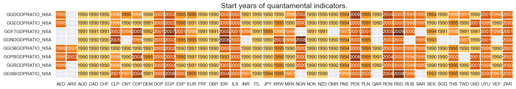
Real-time data of general government balances go back to the 1990s for most developed markets and some emerging market categories. Roughly half of the vintages are actual originally published data, whilst the rest are estimated based on earliest available vintages. The IMF does not estimate net government debt for some EM countries.

For the explanation of currency symbols, which are related to currency areas or countries for which categories are available, please view Appendix 2 .

xcatx = main
cidx = cids_exp

dfx = msm.reduce_df(df, xcats=xcatx, cids=cidx)
dfs = msm.check_startyears(
    dfx,
)
msm.visual_paneldates(dfs, size=(20, 3))

print("Last updated:", date.today())

Last updated: 2025-02-27

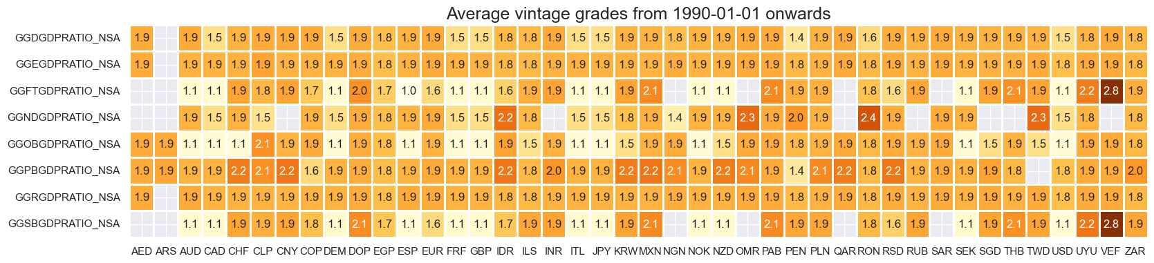
Vintage grading has been mixed, with top grades mainly achieved for the time after 2000.

plot = msp.heatmap_grades(
    df,
    xcats=main,
    cids=cids_exp,
    size=(19, 4),
    title=f"Average vintage grades from {start_date} onwards",
)

cat = ['GGSBGDPRATIO_NSA']
cids = list(set(cids))
msp.view_ranges(
    df,
    xcats=cat,
    cids=cids_exp,
    val="eop_lag",
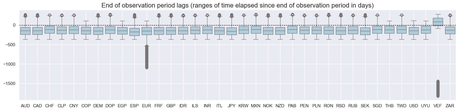
    title="End of observation period lags (ranges of time elapsed since end of observation period in days)",
    start=start_date,
    kind="box",
    size=(16, 4),
)
msp.view_ranges(
    df,
    xcats=cat,
    cids=cids_exp,
    val="mop_lag",
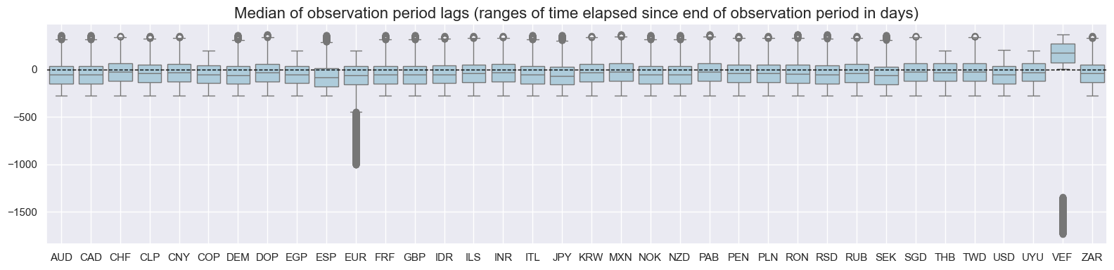
    title="Median of observation period lags (ranges of time elapsed since end of observation period in days)",
    start=start_date,
    kind="box",
    size=(16, 4),
)

History

# for convenience we provide a dictionary to translate the tickers into more readable labels
lab_dict = {
    "GGOBGDPRATIO_NSA": "Overall balance, current year",
    "GGPBGDPRATIO_NSA": "Primary balance, current year",
    "GGSBGDPRATIO_NSA": "Structural balance, current year", 
    "GGRGDPRATIO_NSA": "General government revenues, current year",
    "GGEGDPRATIO_NSA": "General government expenditures, current year", 
    "GGDGDPRATIO_NSA": "General government debt, % of GDP: gross current year",
    "GGNDGDPRATIO_NSA": "General government debt, % of GDP: net current year",
    "GGFTGDPRATIO_NSA": "Fiscal thrust, % of GDP: current year",
    "GGOBGDPRATIONY_NSA": "Overall balance, next year",
    "GGPBGDPRATIONY_NSA": "Primary balance, next year",
    "GGSBGDPRATIONY_NSA": "Structural balance, next year", 
    "GGRGDPRATIONY_NSA": "General government revenues, next year",
    "GGEGDPRATIONY_NSA": "General government expenditures, next year",
    "GGDGDPRATIONY_NSA": "General government debt, % of GDP: gross next year",
    "GGNDGDPRATIONY_NSA": "General government debt, % of GDP: net next year",
    "GGFTGDPRATIONY_NSA": "Fiscal thrust, % of GDP: next year",
    "GGOBGDPRATIOPY_NSA": "Overall balance, previous year",
    "GGPBGDPRATIOPY_NSA": "Primary balance, previous year",
    "GGSBGDPRATIOPY_NSA": "Structural balance, previous year",
    "GGRGDPRATIOPY_NSA": "General government revenues, previous year",
    "GGEGDPRATIOPY_NSA": "General government expenditures, previous year",
    "GGDGDPRATIOPY_NSA": "General government debt, % of GDP: gross previous year",
    "GGNDGDPRATIOPY_NSA": "General government debt, % of GDP: net previous year", 
    "GGFTGDPRATIOPY_NSA": "Fiscal thrust, % of GDP: previous year",
}

Overall and primary balance ratios

Government balances have typically been in a range of +10% to -10% of GDP. Overall balances since 1992 have posted deficits of 1-5% of GDP for most countries. Primary balances averaged close to zero for many countries.

xcatx = ["GGOBGDPRATIO_NSA", "GGPBGDPRATIO_NSA"]
filt_lab_dict = {k: v for k, v in lab_dict.items() if k in xcatx}
cidx = list(set(cids) - set(cids_frontier))

msp.view_ranges(
    df,
    xcats=xcatx,
    cids=cidx,
    sort_cids_by="mean",
    start="1991-01-01",
    title="Means and standard deviations of general government balance ratios (% of GDP) since 1991",
    xcat_labels=[filt_lab_dict.get(x, x) for x in xcatx],
    kind="bar",
    size=(16, 8),
)

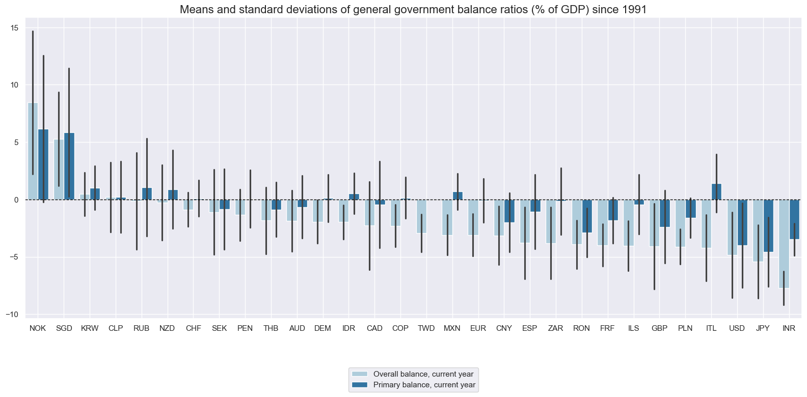
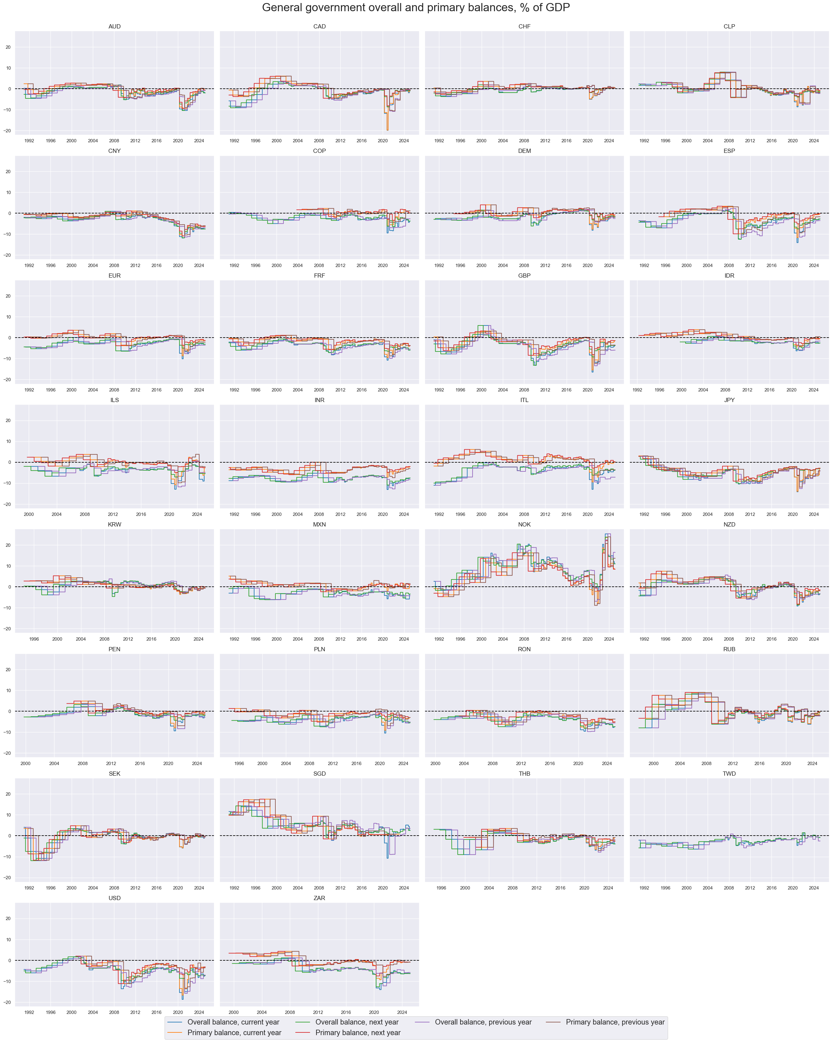
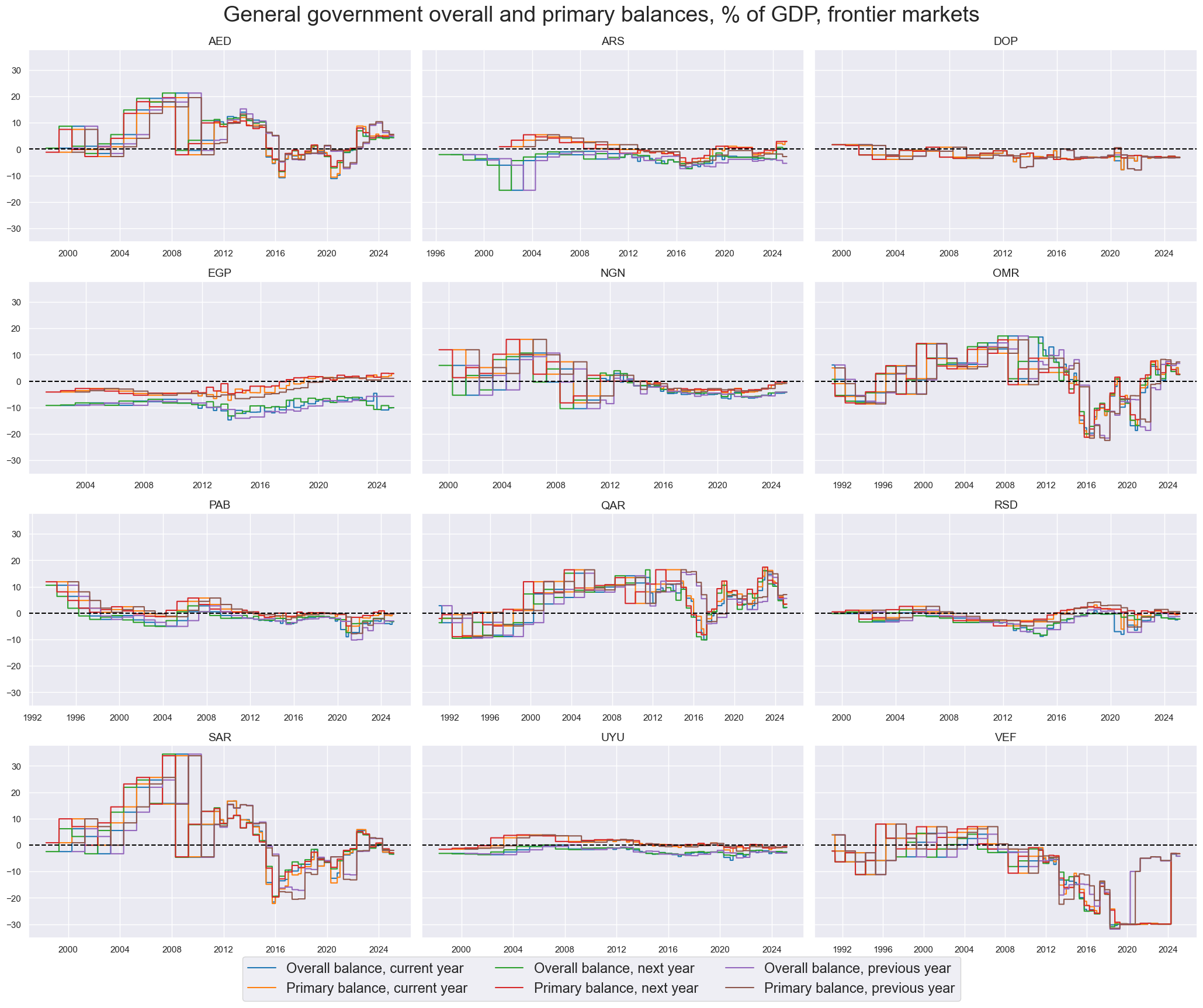
For many countries, government balances posted have pronounced cyclical swings, deteriorating after financial crises and recessions and recovering thereafter. This illustrates that fiscal policy had a tendency to smooth growth performance. Most conspicuously, all countries ran sizable deficits during the COVID-19 pandemic.

xcatx = ["GGOBGDPRATIO_NSA", 
         "GGPBGDPRATIO_NSA", 
         "GGOBGDPRATIONY_NSA", 
         "GGPBGDPRATIONY_NSA", 
         "GGOBGDPRATIOPY_NSA", 
         "GGPBGDPRATIOPY_NSA"]

cidx = sorted(list(set(cids) - set(cids_frontier)))

msp.view_timelines(
    df,
    xcats=xcatx,
    cids=cidx,
    start="1991-01-01",
    title="General government overall and primary balances, % of GDP",
    title_fontsize=27,
    legend_fontsize=17,
    xcat_labels=lab_dict,
    ncol=4,
    same_y=True,
    size=(16, 8),
    all_xticks=True,
)

xcatx = ["GGOBGDPRATIO_NSA", 
         "GGPBGDPRATIO_NSA", 
         "GGOBGDPRATIONY_NSA", 
         "GGPBGDPRATIONY_NSA", 
         "GGOBGDPRATIOPY_NSA", 
         "GGPBGDPRATIOPY_NSA"]

cidx = cids_frontier

msp.view_timelines(
    df,
    xcats=xcatx,
    cids=cidx,
    start="1991-01-01",
    title="General government overall and primary balances, % of GDP, frontier markets",
    title_fontsize=27,
    legend_fontsize=17,
    xcat_labels=lab_dict,
    same_y=True,
    size=(16, 8),
    all_xticks=True,
)

Structural balance ratios

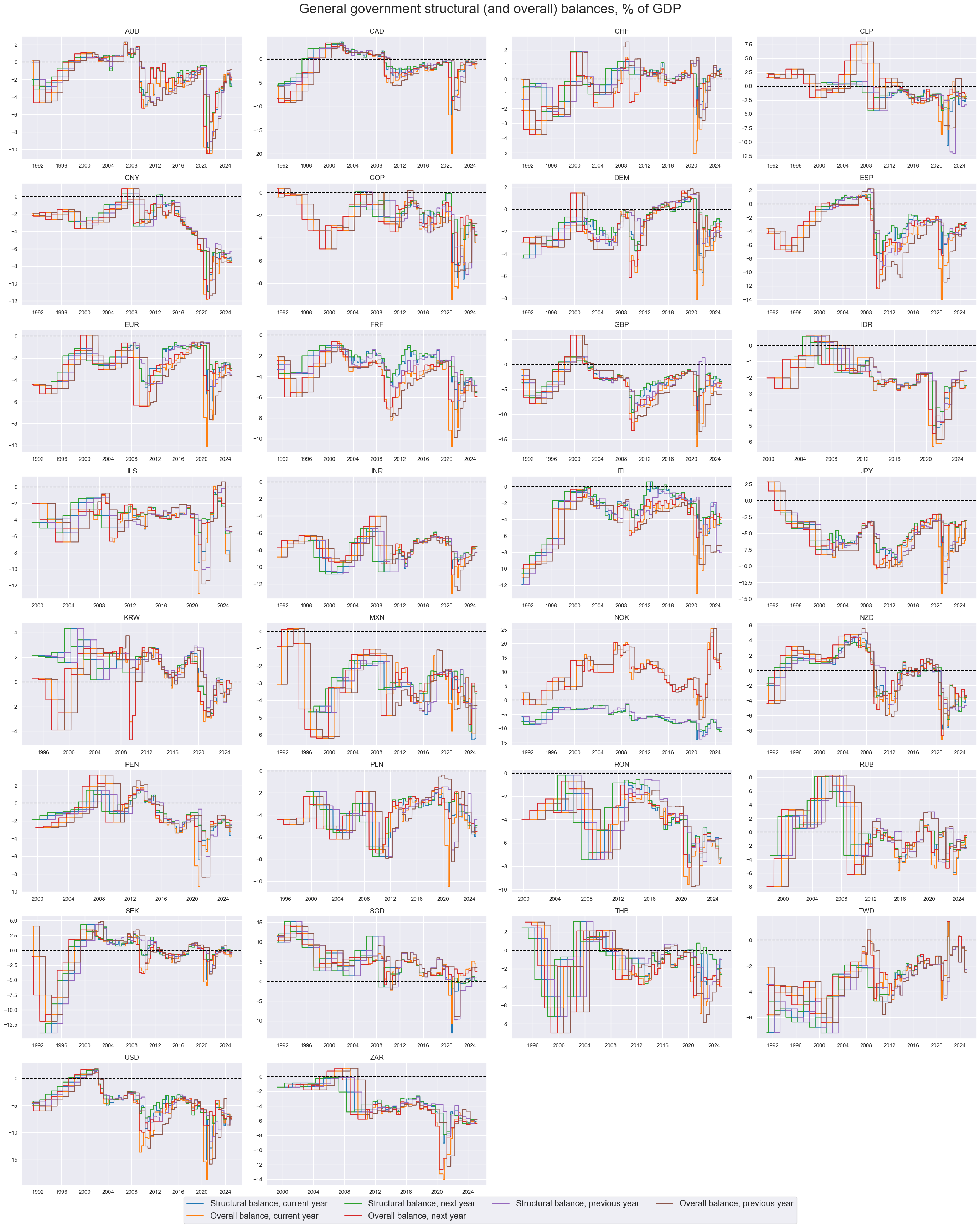
For most countries, structural balances have fluctuated around the headline balance, depending largely on financial, economic and commodity cycles. Norway is a notable exception, whose large surplus has not been classified as structural according to IMF methodology.

xcatx = ["GGSBGDPRATIO_NSA", 
         "GGOBGDPRATIO_NSA", 
         "GGSBGDPRATIONY_NSA", 
         "GGOBGDPRATIONY_NSA", 
         "GGSBGDPRATIOPY_NSA", 
         "GGOBGDPRATIOPY_NSA"]

cidx = sorted(list(set(cids) - set(cids_frontier)))

msp.view_timelines(
    df,
    xcats=xcatx,
    cids=cidx,
    start="1991-01-01",
    title="General government structural (and overall) balances, % of GDP",
    title_fontsize=27,
    legend_fontsize=17,
    xcat_labels=lab_dict,
    ncol=4,
    same_y=False,
    size=(16, 8),
    all_xticks=True,
)

Revenue and expenditure ratios

General government revenue and expenditure ratios have mostly averaged between 20% and 50% of GDP across countries.

xcatx = ["GGRGDPRATIO_NSA", "GGEGDPRATIO_NSA"]
filt_lab_dict = {k: v for k, v in lab_dict.items() if k in xcatx}
cidx = cids

msp.view_ranges(
    df,
    xcats=xcatx,
    cids=cidx,
    sort_cids_by="mean",
    start="1991-01-01",
    title="Means and standard deviations of general government flows (as % of GDP) since 1991",
    xcat_labels=[filt_lab_dict.get(x, x) for x in xcatx],
    kind="bar",
    size=(16, 8),
)

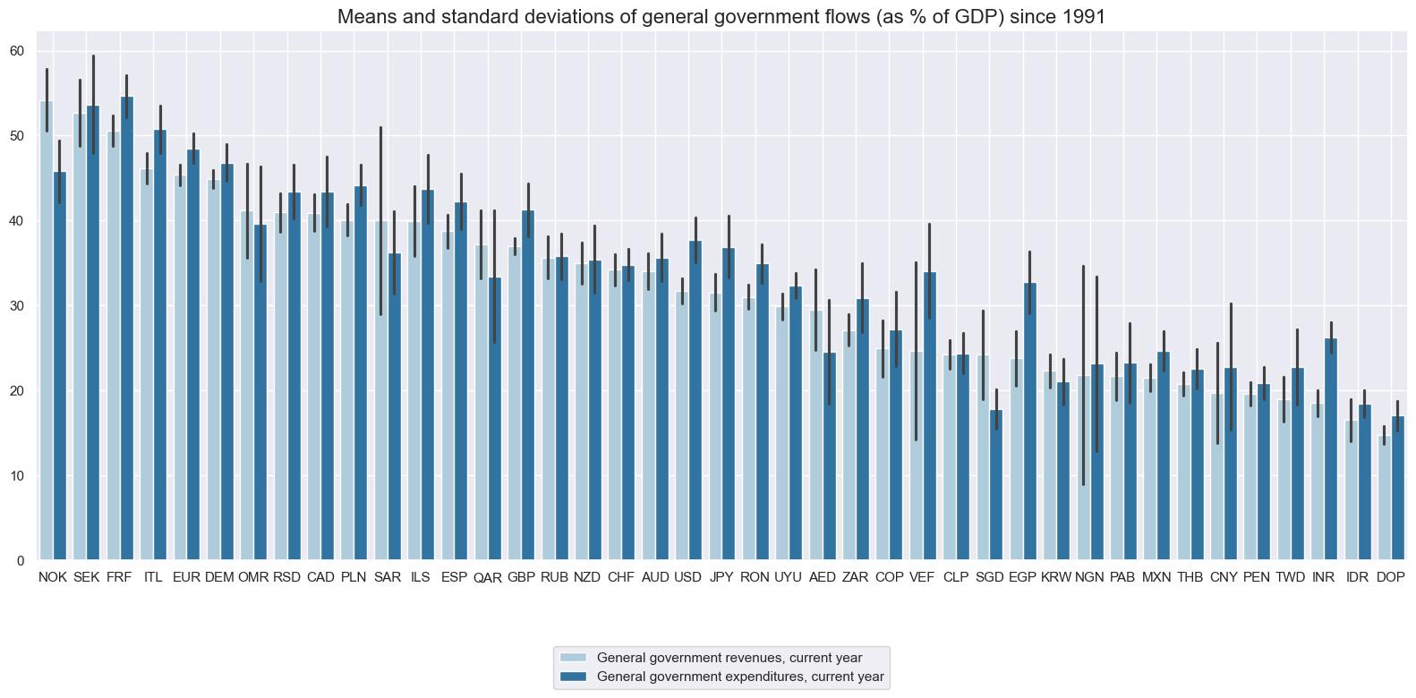
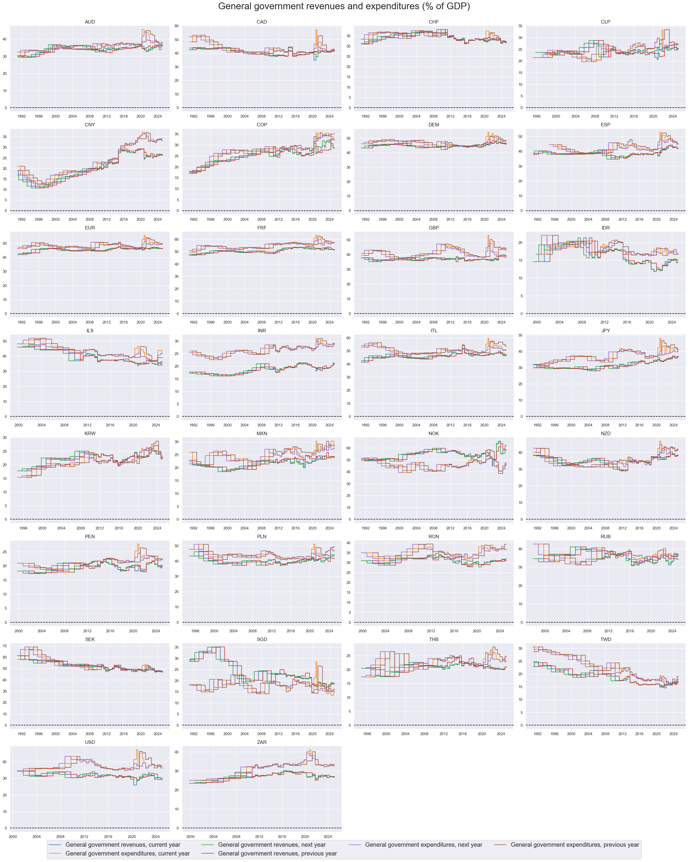
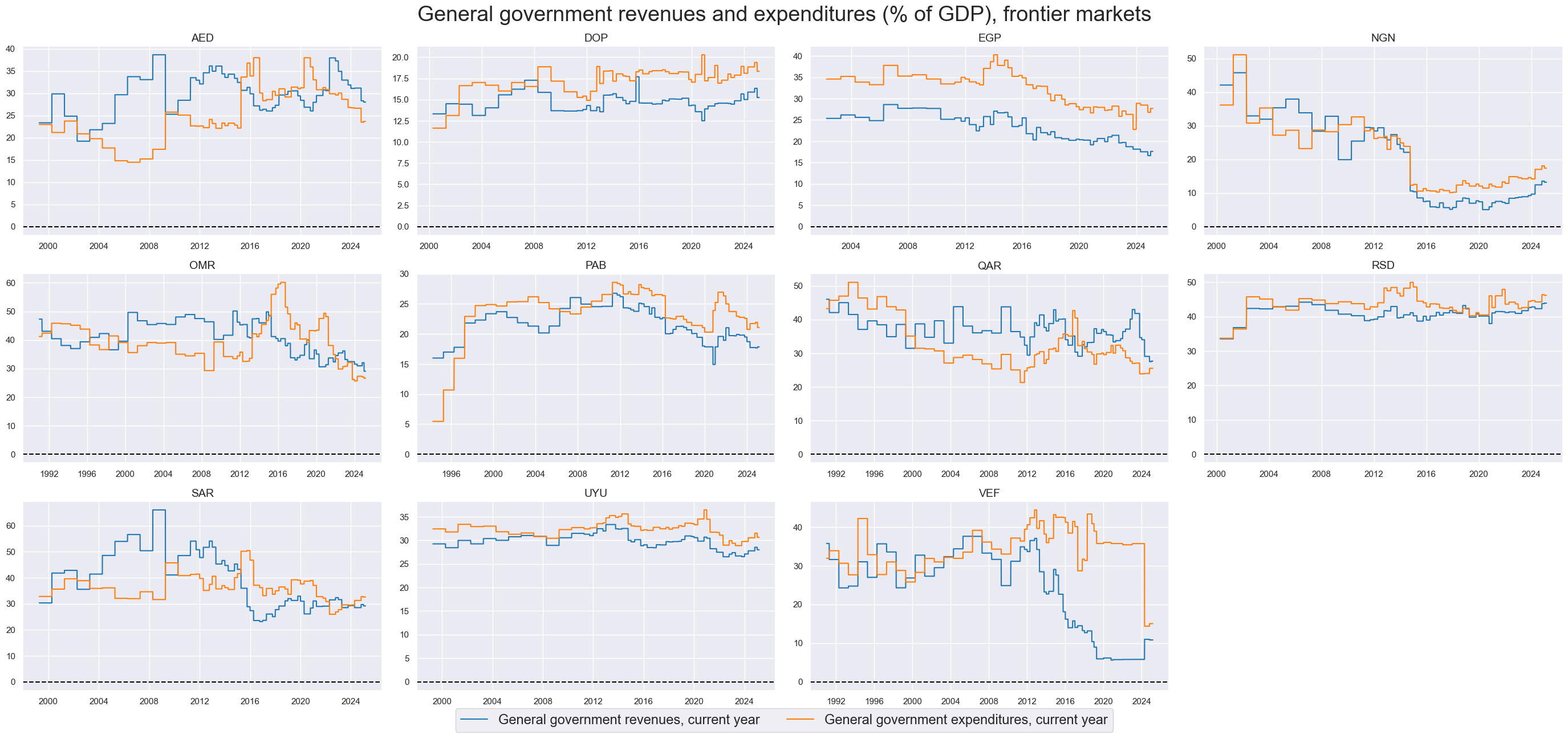
Secular trends in the size of the general government flows to GDP have been very different across countries.

During recessions and recoveries, revenues and expenditure ratios often shift in opposite directions, indicating a counter-cyclical fiscal stance, whether through active policy or automatic stabilizers.

xcatx = ["GGRGDPRATIO_NSA", 
         "GGEGDPRATIO_NSA", 
         "GGRGDPRATIONY_NSA", 
         "GGRGDPRATIOPY_NSA", 
         "GGEGDPRATIONY_NSA", 
         "GGEGDPRATIOPY_NSA"
        ]

cidx = sorted(list(set(cids) - set(cids_frontier)))

msp.view_timelines(
    df,
    xcats=xcatx,
    cids=cidx,
    start="1991-01-01",
    title="General government revenues and expenditures (% of GDP)",
    title_fontsize=27,
    legend_fontsize=17,
    xcat_labels= lab_dict,
    ncol=4,
    same_y=False,
    size=(16, 8),
    all_xticks=True,
)

xcatx = ["GGRGDPRATIO_NSA", "GGEGDPRATIO_NSA"]
cidx = cids_frontier

msp.view_timelines(
    df,
    xcats=xcatx,
    cids=cidx,
    start="1991-01-01",
    title="General government revenues and expenditures (% of GDP), frontier markets",
    title_fontsize=27,
    legend_fontsize=17,
    xcat_labels=lab_dict,
    ncol=4,
    same_y=False,
    size=(16, 8),
    all_xticks=True,
)

General government debt ratios

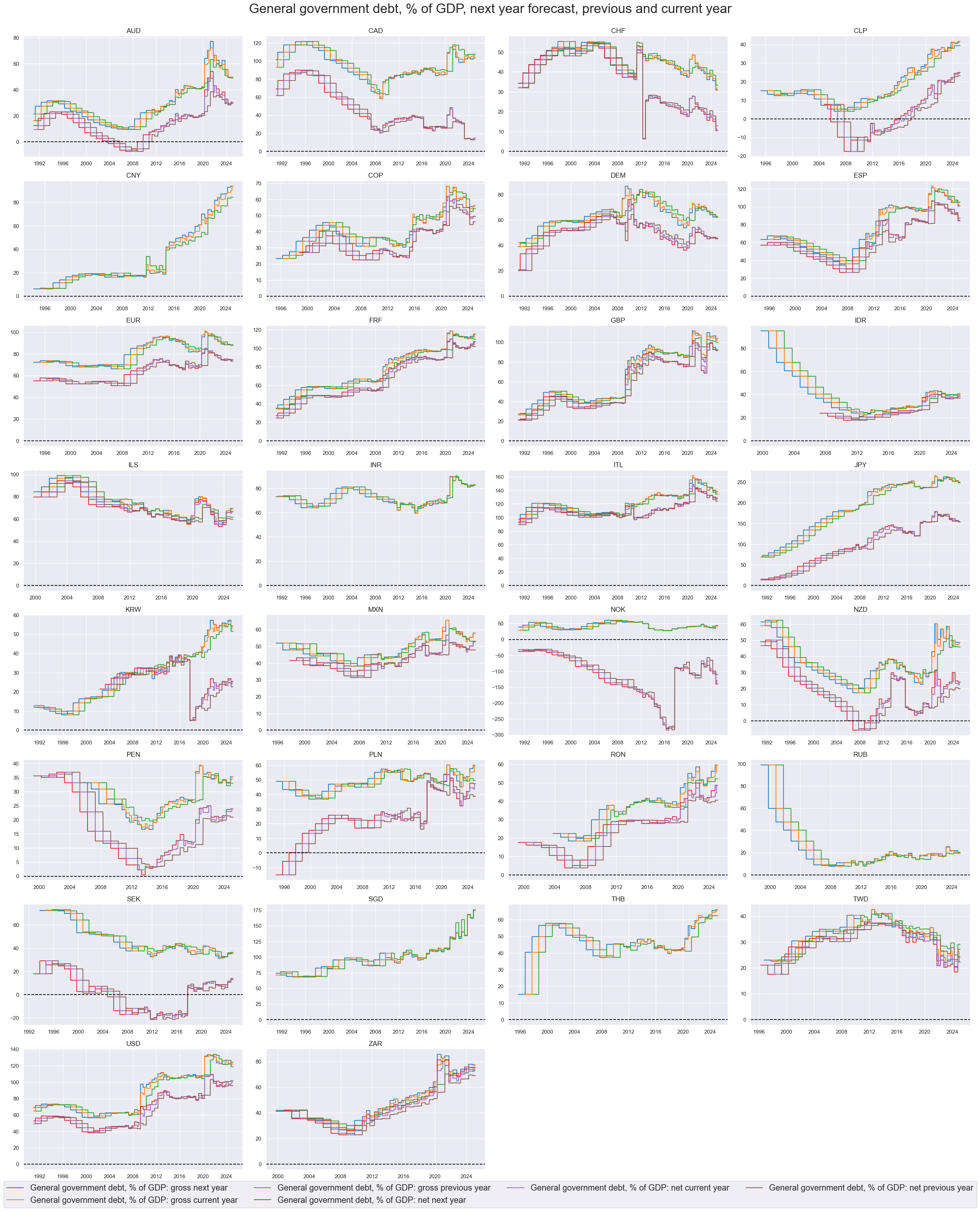
Gross government debt ratios have typically between 30% and 100% of GDP since the early 1990s. There have been two notable outliers. Japan’s debt statistics had exceeded 250% of GDP by the 2020s, whilst Norway’s substantial negative debt ratio is attributed to its sovereign wealth fund.

xcatx = ["GGDGDPRATIO_NSA", "GGNDGDPRATIO_NSA"]
filt_lab_dict = {k: v for k, v in lab_dict.items() if k in xcatx}
cidx = cids

msp.view_ranges(
    df,
    xcats=xcatx,
    cids=cidx,
    sort_cids_by="mean",
    start="1991-01-01",
    kind="bar",
    title="Means and standard deviations of general government debt (as % of GDP) since 1991",
    xcat_labels=[filt_lab_dict.get(x, x) for x in xcatx],
    size=(16, 8),
)

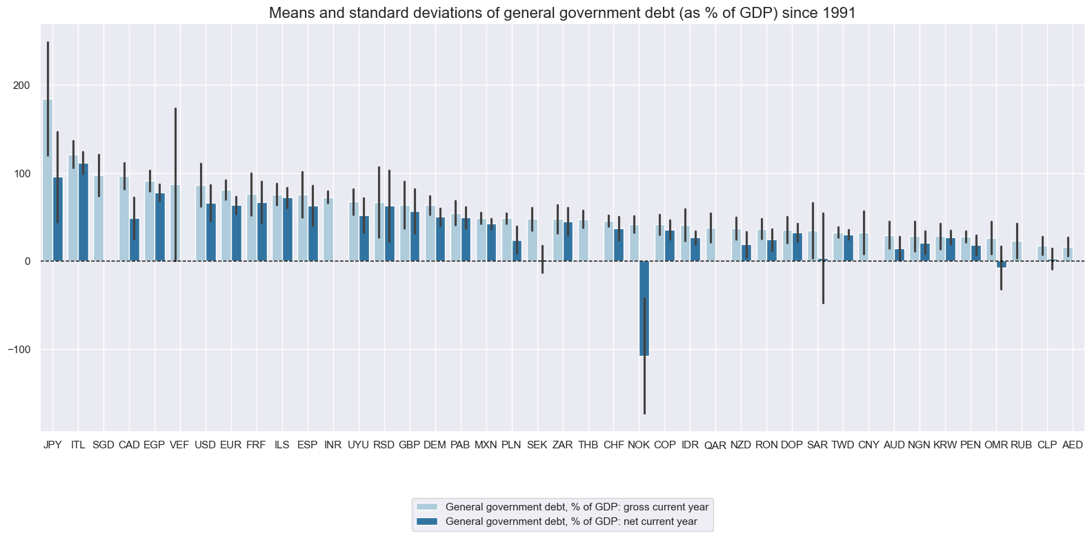
Long-term trends in government debt ratios have been quite diverse across countries in past decades. Most developed countries posted an upward drift, while many EM countries reduced debt ratios in the 2000s and early 2010s. Both the great financial crisis and the COVID-19 pandemic triggered notable increases in debt ratios.

Real-time measures of net debt ratios have displayed a greater proclivity to instability overtime, due typically to methodological adjustments. Few countries have achieved negative net debt ratios. Norway has been a notable example.

xcatx = ["GGDGDPRATIONY_NSA", 
         "GGDGDPRATIO_NSA", 
         "GGDGDPRATIOPY_NSA",
         "GGNDGDPRATIONY_NSA", 
         "GGNDGDPRATIO_NSA", 
         "GGNDGDPRATIOPY_NSA"]


cidx = sorted(list(set(cids) - set(cids_frontier)))

msp.view_timelines(
    df,
    xcats=xcatx,
    cids=cidx,
    start="1991-01-01",
    title="General government debt, % of GDP, next year forecast, previous and current year",
    title_fontsize=27,
    legend_fontsize=17,
    xcat_labels=lab_dict,
    ncol=4,
    same_y=False,
    size=(16, 8),
    all_xticks=True,
)

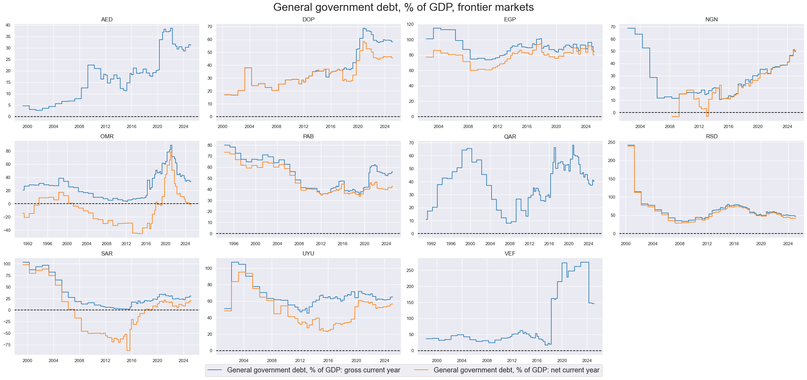
xcatx = ["GGDGDPRATIO_NSA", "GGNDGDPRATIO_NSA"]
cidx = cids_frontier

msp.view_timelines(
    df,
    xcats=xcatx,
    cids=cidx,
    start="1991-01-01",
    title="General government debt, % of GDP, frontier markets",
    title_fontsize=27,
    legend_fontsize=17,
    xcat_labels=lab_dict,
    ncol=4,
    same_y=False,
    size=(16, 8),
    all_xticks=True,
)

Fiscal thrust

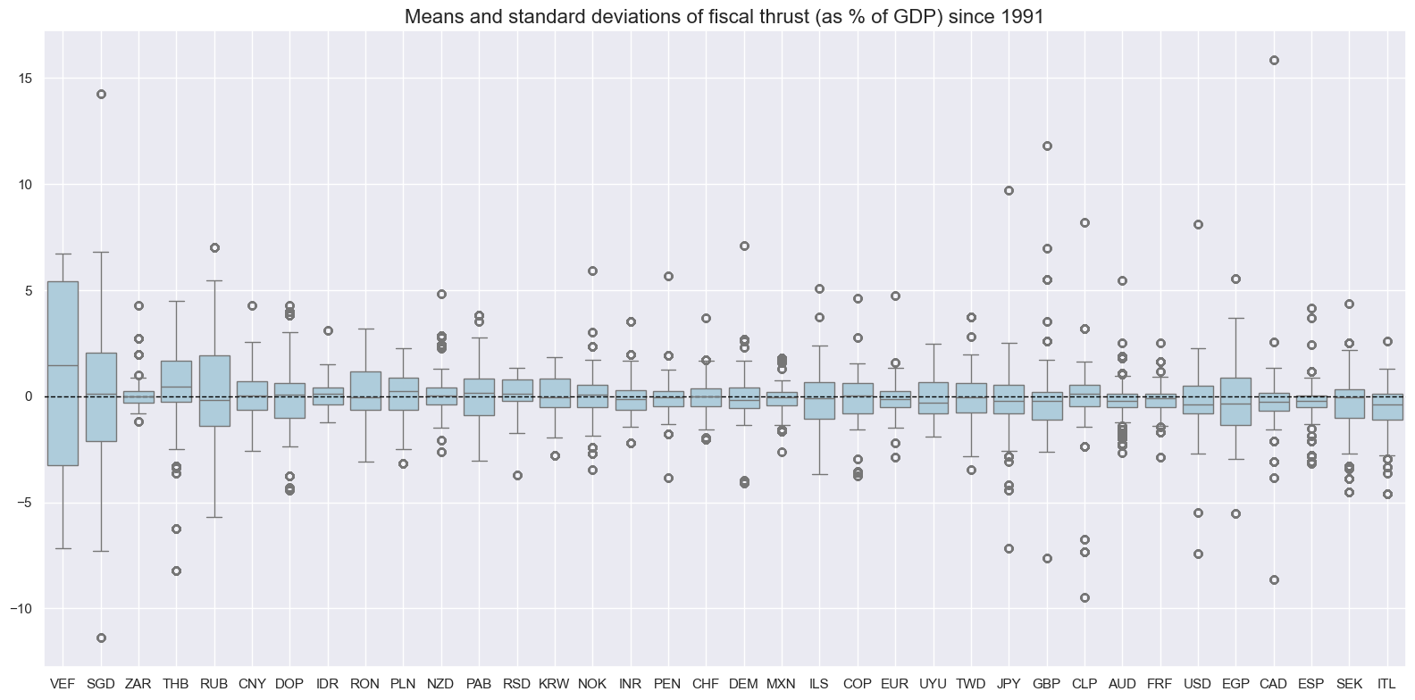
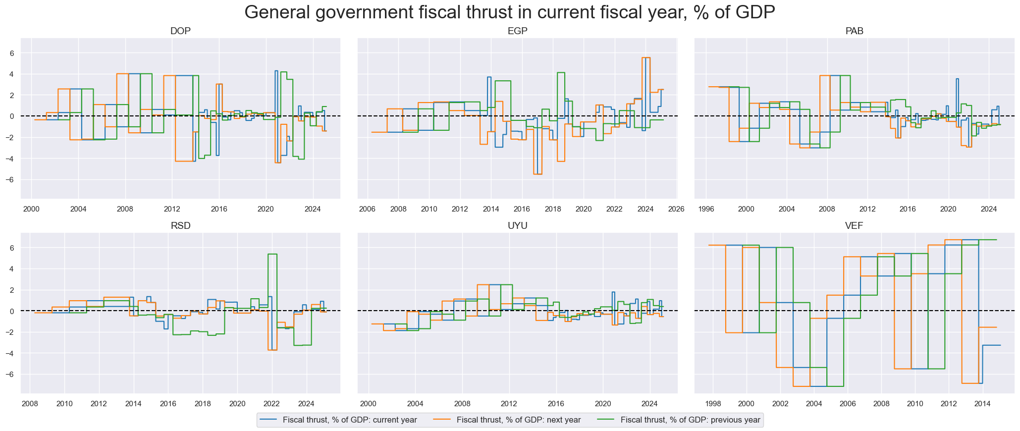
Typical fiscal thrust has been contained in a range of +/- 1% of GDP for most countries and years, but has witnessed many outlier values. The COVID-19 pandemic coerced much greater temporary fiscal stimulus in many countries.

xcatx = ["GGFTGDPRATIO_NSA"]
cidx = cids

msp.view_ranges(
    df,
    xcats=xcatx,
    cids=cidx,
    sort_cids_by="mean",
    start="1991-01-01",
    kind="box",
    title="Means and standard deviations of fiscal thrust (as % of GDP) since 1991",
    size=(16, 8),
)

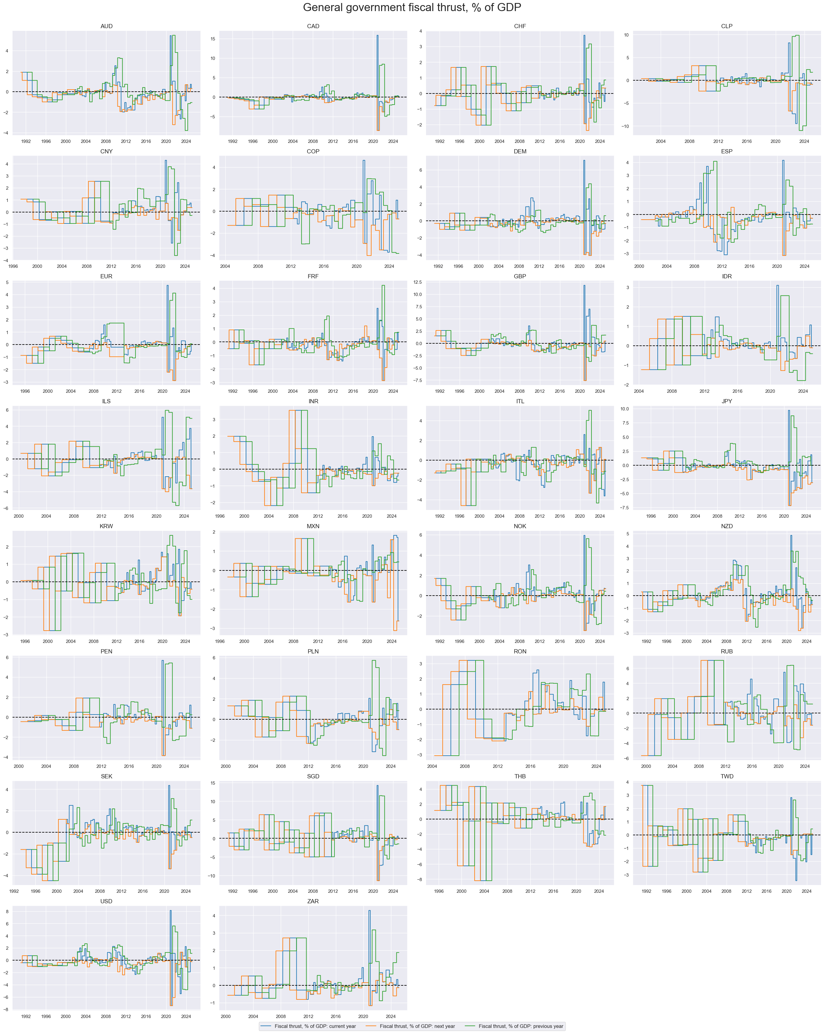
Fiscal thrust has been historically volatile, reflecting changes in fiscal policy as much as changes in economic conditions.

xcatx = ["GGFTGDPRATIO_NSA", "GGFTGDPRATIONY_NSA", "GGFTGDPRATIOPY_NSA"]
cidx = sorted(list(set(cids) - set(cids_frontier)))

msp.view_timelines(
    df,
    xcats=xcatx,
    cids=cidx,
    start="1991-01-01",
    title="General government fiscal thrust, % of GDP",
    title_fontsize=27,
    same_y=False,
    ncol=4,
    size=(16, 8),
    xcat_labels=lab_dict,
    all_xticks=True,
)

xcatx = ["GGFTGDPRATIO_NSA", "GGFTGDPRATIONY_NSA", "GGFTGDPRATIOPY_NSA"]
cidx = cids_frontier

msp.view_timelines(
    df,
    xcats=xcatx,
    cids=cidx,
    start="1991-01-01",
    title="General government fiscal thrust in current fiscal year, % of GDP",
    title_fontsize=27,
    xcat_labels=lab_dict,
    same_y=True,
    size=(16, 8),
    all_xticks=True,
)

Importance

Research links

“This paper re-examines the impact of fiscal deficits and public debt on long-term interest rates…for a panel of 31 advanced and emerging market economies…Higher deficits and public debt lead to a significant increase in long-term interest rates, with the precise magnitude dependent on initial fiscal, institutional and other structural conditions, as well as spillovers from global financial markets…Large fiscal deficits and public debts are likely to put substantial upward pressures on sovereign bond yields in many advanced economies over the medium term.” Kumar and Baldacci

“Fiscal impulse measures…indicate the changing impact of the budget on the economy. Such measures are intended to provide more accurate indications of whether the budget is becoming more or less expansionary than would just observing moments in the actual budget balance.” Chand

“It is always the joint behavior of monetary and fiscal policies that determine inflation and stabilize debt. While this point might seem obvious…it is easily missed in the classes of models and descriptions of policy typically employed in modern macroeconomic policy analyses…Expectations of fiscal policy are equally important to those of monetary policy in determining prices.” Leeper and Leith

Empirical clues

# Blacklist periods of FX targeting or illiquidity

dfb = df[df["xcat"].isin(["FXTARGETED_NSA", "FXUNTRADABLE_NSA"])].loc[
    :, ["cid", "xcat", "real_date", "value"]
]
dfba = (
    dfb.groupby(["cid", "real_date"])
    .aggregate(value=pd.NamedAgg(column="value", aggfunc="max"))
    .reset_index()
)
dfba["xcat"] = "FXBLACK"
fxblack = msp.make_blacklist(
    dfba, "FXBLACK"
)  # dictionary of periods of FX targeting or illiquidity
fxblack

{'CHF': (Timestamp('2011-10-03 00:00:00'), Timestamp('2015-01-30 00:00:00')),
 'CNY': (Timestamp('1999-01-01 00:00:00'), Timestamp('2025-02-26 00:00:00')),
 'ILS': (Timestamp('1999-01-01 00:00:00'), Timestamp('2005-12-30 00:00:00')),
 'INR': (Timestamp('1999-01-01 00:00:00'), Timestamp('2004-12-31 00:00:00')),
 'PEN': (Timestamp('2021-07-01 00:00:00'), Timestamp('2021-07-30 00:00:00')),
 'RON': (Timestamp('1999-01-01 00:00:00'), Timestamp('2005-11-30 00:00:00')),
 'RUB_1': (Timestamp('1999-01-01 00:00:00'), Timestamp('2005-11-30 00:00:00')),
 'RUB_2': (Timestamp('2022-02-01 00:00:00'), Timestamp('2025-02-26 00:00:00')),
 'SGD': (Timestamp('1999-01-01 00:00:00'), Timestamp('2025-02-26 00:00:00')),
 'THB': (Timestamp('2007-01-01 00:00:00'), Timestamp('2008-11-28 00:00:00'))}

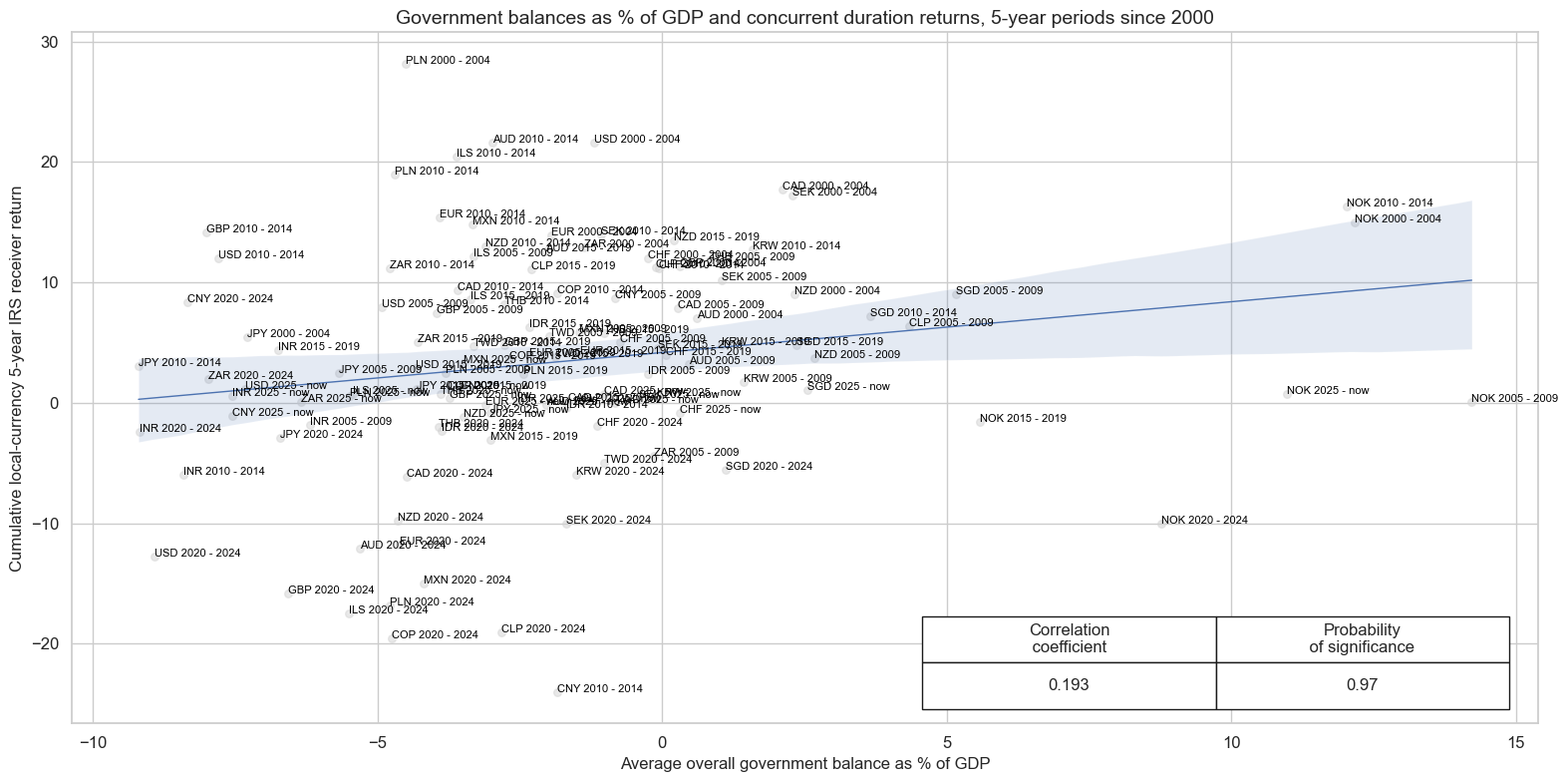
There is evidence that stronger reported general government balances, in terms of lower deficits or higher surpluses have coincided with and entailed better fixed income returns since 2000 across developed and emerging countries. The relation holds across all types of government balances, but predictive power has been strongest for primary balances.

cidx = list(set(cids) - set(["PEN", "RON", "RUB"] + cids_dmec) - set(cids_frontier))  # tradable countries

cr = msp.CategoryRelations(
    df,
    xcats=["GGOBGDPRATIO_NSA", "DU05YXR_NSA"],
    cids=cidx,
    freq="A",
    lag=0,
    xcat_aggs=["mean", "sum"],
    start="2000-01-01",
    years=5,
)

cr.reg_scatter(
    title="Government balances as % of GDP and concurrent duration returns, 5-year periods since 2000",
    labels=True,
    coef_box="lower right",
    ylab="Cumulative local-currency 5-year IRS receiver return",
    size=(16, 8),
    xlab="Average overall government balance as % of GDP",
)

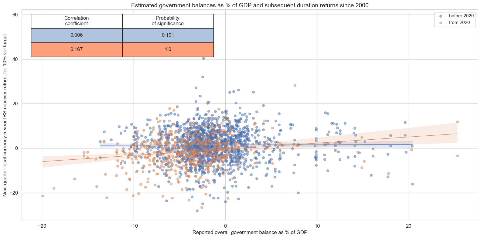
Formally, reported general government balances have also been predictors of subsequent duration returns. However, that relation has not been stable across time and concentrated on the 2020s.

cidx = list(set(cids) - set(["PEN", "RON", "RUB"] + cids_dmec) - set(cids_frontier))

cr = msp.CategoryRelations(
    df,
    xcats=["GGOBGDPRATIO_NSA", "DU05YXR_VT10"],
    cids=cidx,
    freq="Q",
    lag=1,
    xcat_aggs=["last", "sum"],
    start="2000-01-01",
    years=None,
)

cr.reg_scatter(
    title="Estimated government balances as % of GDP and subsequent duration returns since 2000",
    labels=False,
    separator=2020,
    size=(16, 8),
    coef_box="upper left",
    ylab="Next quarter local-currency 5-year IRS receiver return, for 10% vol target",
    xlab="Reported overall government balance as % of GDP",
)

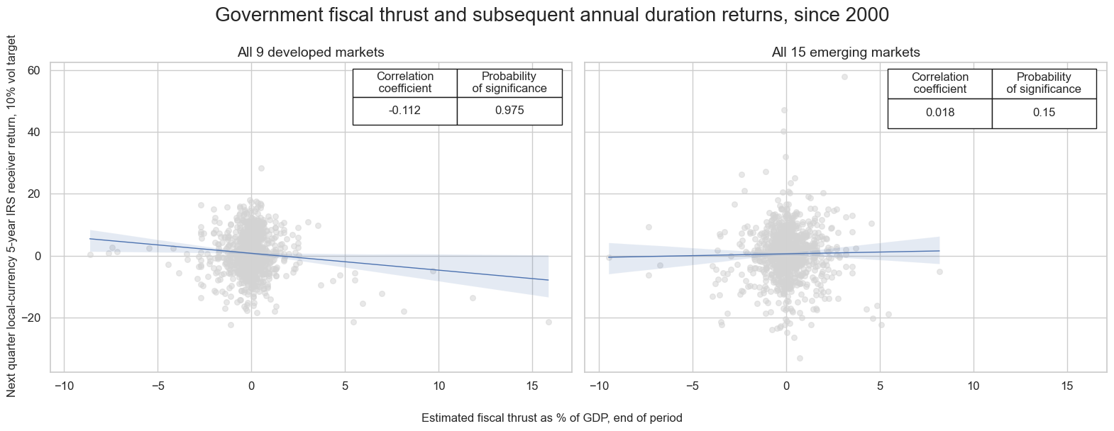
There is better evidence suggesting a negative correlation exists between average fiscal thrust and next quarters’ local currency 5-year duration returns. The relation has been subtle but relatively stable. Fiscal thrust indicators are meaningful mainly for developed markets.

# specify the signals, targets and currencies for the analysis
sigx_irs = {
    "GGFTGDPRATIO_NSA": "Fiscal thrust, % of GDP: current year", 
}

targx_irs = {
    "DU05YXR_VT10": "Local-currency 5-year IRS receiver return, 10% vol target",

}

cidx_dict_irs = {
    f"All {len(set(cids_dm) - set(cids_dmec))} developed markets": list(set(cids_dm) - set(cids_dmec)),
    f"All {len(set(cids_em) - set (['PEN', 'RON']))} emerging markets": list(set(cids_em) - set (['PEN', 'RON'])) # data for PEN and RON not available
}

# Iterate through the mapped currency areas: 
cr = {}
for cid_name, cid_list in cidx_dict_irs.items(): 
     
    cr[f"cr_{cid_name}"] = msp.CategoryRelations(
        df,
        xcats=[", ".join(sigx_irs.keys()), ", ".join(targx_irs.keys())],
        cids=cid_list,  
        freq="Q",
        lag=1,
        xcat_aggs=["last", "sum"],
        blacklist=fxblack,
        start="2000-01-01",
        
    )
#Combine all CategoryRelations instances for plotting
all_cr_instances = [
    cr[f"cr_{cid_name}"]
    for cid_name in cidx_dict_irs.keys() 
]

# Dynamically create subplot titles 
subplot_titles = [
    f"{cid_name}"  # Use the descriptive keys from cidx directly
    for cid_name in cidx_dict_irs.keys()
]
# plot side by side all the CategoryRelations instances
msv.multiple_reg_scatter(
        all_cr_instances,
        title="Government fiscal thrust and subsequent annual duration returns, since 2000" ,
        xlab="Estimated fiscal thrust as % of GDP, end of period",
        ylab="Next quarter local-currency 5-year IRS receiver return, 10% vol target",
        ncol=2,
        nrow=1,
        figsize=(16, 6),
        prob_est="map",
        subplot_titles = subplot_titles,
        coef_box="upper right",
   
     )

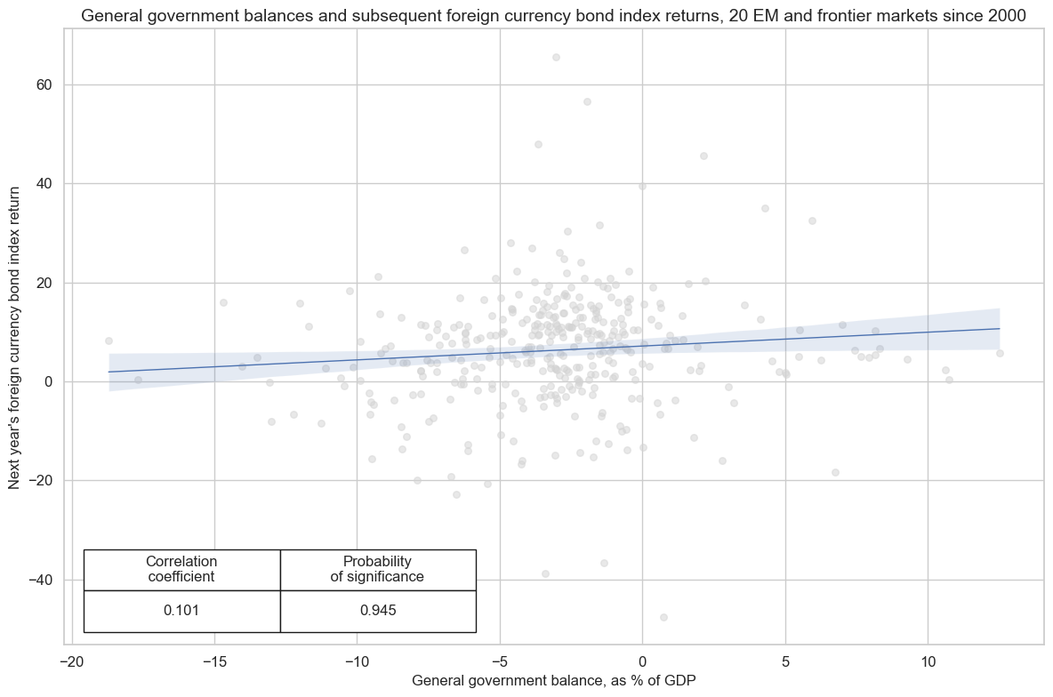
For the wider emerging markets country group, consisting of advanced EM countries and the frontier markets, there is pervasive evidence that information states of strong general government balances predict better foreign-currency sovereign bond returns. Large deficits have often been followed by negative returns. Predictive relations hold for overall and primary government balances and at a quarterly or even annual horizon.

cidx = cids_em + cids_frontier
xcatx = ["GGOBGDPRATIO_NSA", "FCBIR_NSA"]
cidx = msm.common_cids(df, xcats = xcatx)

cr = msp.CategoryRelations(
    df,
    xcats=["GGOBGDPRATIO_NSA", "FCBIR_NSA"],
    cids=cidx,
    freq="A",
    lag=1,
    xcat_aggs=["last", "sum"],
    start="2000-01-01",
    blacklist=fxblack,
    years=None,
)

cr.reg_scatter(
    title=f"General government balances and subsequent foreign currency bond index returns, {len(cidx)} EM and frontier markets since 2000",
    labels=False,
    coef_box="lower left",
    ylab="Next year's foreign currency bond index return",
    xlab="General government balance, as % of GDP",
)

Appendices

Appendix 1: Source data notes

IMF data is taken from two sources: the IMF Fiscal Monitor and the World Economic Outlook. The IMF publishes the Fiscal Monitor twice a year, usually in April and October. It also publishes the World Economic Outlook at least twice a year. It tends to be released a couple of days before the IMF Fiscal Monitor publication. The government finance data in the IMF Fiscal Monitor match that published in the World Economic Outlook.

Detailed notes are provided by the IMF on various terms used in the indicator definitions.

• Primary balance: https://www.imf.org/external/np/fad/histdb

• Structural balance: https://www.imf.org/external/np/fad/strfiscbal/index.htm

• Revenues: https://www.imf.org/external/pubs/ft/gfs/manual/pdf/ch5.pdf

• Expenditures: https://www.imf.org/-/media/Files/Publications/fiscal-monitor/2022/October/English/msa.ashx

The notes on government balance ratios (see primary balance and structural balance notes) apply to fiscal thrust.

Appendix 2: Currency symbols

The word ‘cross-section’ refers to currencies, currency areas or economic areas. In alphabetical order, these are AED (Emirates dirham), ARS (Argentine Peso), AUD (Australian dollar), BRL (Brazilian real), CAD (Canadian dollar), CHF (Swiss franc), CLP (Chilean peso), CNY (Chinese yuan renminbi), COP (Colombian peso), CZK (Czech Republic koruna), DEM (German mark), DOP (Dominican Peso), EGP (Egyptian Pound), ESP (Spanish peseta), EUR (Euro), FRF (French franc), GBP (British pound), HKD (Hong Kong dollar), HUF (Hungarian forint), IDR (Indonesian rupiah), ITL (Italian lira), JPY (Japanese yen), KRW (Korean won), MXN (Mexican peso), MYR (Malaysian ringgit), NGN (Nigerian Naira), NLG (Dutch guilder), NOK (Norwegian krone), NZD (New Zealand dollar), OMR (Omani Rial), PAB (Panamanian balboa), PEN (Peruvian sol), PHP (Phillipine peso), PLN (Polish zloty), QAR (Qatari riyal), RON (Romanian leu), RSD (Serbian Dinar), RUB (Russian ruble), SAR (Saudi riyal), SEK (Swedish krona), SGD (Singaporean dollar), THB (Thai baht), TRY (Turkish lira), TWD (Taiwanese dollar), USD (U.S. dollar), UYU (Uruguayan peso), VEF (Venezuelan bolívar), ZAR (South African rand).