Equity trading strategies with macro and random forests

The random forest is a machine learning model composed of many different “decision tree” models. Decision trees are sequences of “if-else” statements, where “learning” in the regression case corresponds to learning good decision rules from data. The random forest constructs each of these trees to, hopefully, be both reasonable forecasters and be as uncorrelated with one another as possible. The average prediction made by the trees is the prediction made by the random forest.

Get packages and JPMaQS data

Packages

import os
import numpy as np
import pandas as pd
import matplotlib.pyplot as plt

from macrosynergy.download import JPMaQSDownload
import macrosynergy.management as msm
import macrosynergy.panel as msp
import macrosynergy.pnl as msn
import macrosynergy.signal as mss
import macrosynergy.learning as msl
import macrosynergy.visuals as msv

from sklearn.linear_model import LinearRegression
from sklearn.ensemble import RandomForestRegressor
from sklearn.pipeline import Pipeline
from sklearn.metrics import make_scorer

from timeit import default_timer as timer
from datetime import timedelta, date, datetime

import warnings

from IPython.display import HTML

warnings.filterwarnings("ignore")

Previously prepared quantamental categories

# Import data from csv file created preparation notebook
# https://macrosynergy.com/academy/notebooks/sectoral-equity-indicators/

INPUT_PATH = os.path.join(os.getcwd(), r"../../../equity_sectoral_notebook_data.csv")

df_csv = pd.read_csv(INPUT_PATH, index_col=0)
df_csv["real_date"] = pd.to_datetime(df_csv["real_date"]).dt.date

df_csv = msm.utils.standardise_dataframe(df_csv)
df_csv = df_csv.sort_values(["cid", "xcat", "real_date"])

# Equity sector labels and cross sections

sector_labels = {
    "ALL": "All sectors",
    "COD": "Cons. discretionary",
    "COS": "Cons. staples",
    "CSR": "Communication services",
    "ENR": "Energy",
    "FIN": "Financials",
    "HLC": "Healthcare",
    "IND": "Industrials",
    "ITE": "Information tech",
    "MAT": "Materials",
    "REL": "Real estate",
    "UTL": "Utilities",
}
cids_secs = list(sector_labels.keys())

# Equity countries cross sections

cids_eq = [
    "AUD",
    "CAD",
    "CHF",
    "EUR",
    "GBP",
    "ILS",
    "JPY",
    "NOK",
    "NZD",
    "SEK",
    "SGD",
    "USD",
]

# Base category tickes of quantamental categories created by data preparation notebook:
# https://macrosynergy.com/academy/notebooks/sectoral-equity-indicators/

output_growth = [
    # industrial prod
    "XIP_SA_P1M1ML12_3MMA",
    "XIP_SA_P1M1ML12_3MMA_WG",
    # construction
    "XCSTR_SA_P1M1ML12_3MMA",
    "XCSTR_SA_P1M1ML12_3MMA_WG",
    # Excess GDP growth
    "XRGDPTECH_SA_P1M1ML12_3MMA",
    "XRGDPTECH_SA_P1M1ML12_3MMA_WG",
]
private_consumption = [
    # Consumer surveys
    "CCSCORE_SA",
    "CCSCORE_SA_D3M3ML3",
    "CCSCORE_SA_WG",
    "CCSCORE_SA_D3M3ML3_WG",
    
    "XNRSALES_SA_P1M1ML12_3MMA",
    "XRRSALES_SA_P1M1ML12_3MMA",
    "XNRSALES_SA_P1M1ML12_3MMA_WG",
    "XRRSALES_SA_P1M1ML12_3MMA_WG",
    "XRPCONS_SA_P1M1ML12_3MMA",
    "XRPCONS_SA_P1M1ML12_3MMA_WG",    
]
export = [
    "XEXPORTS_SA_P1M1ML12_3MMA",
]
labour_market = [
    "UNEMPLRATE_NSA_3MMA_D1M1ML12",
    "UNEMPLRATE_SA_3MMAv5YMA",
    "UNEMPLRATE_NSA_3MMA_D1M1ML12_WG",
    "UNEMPLRATE_SA_3MMAv5YMA_WG",
    "XEMPL_NSA_P1M1ML12_3MMA",
    "XEMPL_NSA_P1M1ML12_3MMA_WG",
    "XRWAGES_NSA_P1M1ML12",
]
business_surveys = [
    # Manufacturing
    "MBCSCORE_SA",
    "MBCSCORE_SA_D3M3ML3",
    "MBCSCORE_SA_WG",
    "MBCSCORE_SA_D3M3ML3_WG",
    # Services
    "SBCSCORE_SA",
    "SBCSCORE_SA_D3M3ML3",
    "SBCSCORE_SA_WG",
    "SBCSCORE_SA_D3M3ML3_WG",
    # Construction
    "CBCSCORE_SA",
    "CBCSCORE_SA_D3M3ML3",
    "CBCSCORE_SA_WG",
    "CBCSCORE_SA_D3M3ML3_WG",
]
private_credit = [
    "XPCREDITBN_SJA_P1M1ML12",
    "XPCREDITBN_SJA_P1M1ML12_WG",
    # liquidity conditions
    "INTLIQGDP_NSA_D1M1ML1",
    "INTLIQGDP_NSA_D1M1ML6",
]
broad_inflation = [
    # Inflation
    "XCPIC_SA_P1M1ML12",
    "XCPIH_SA_P1M1ML12",
    "XPPIH_NSA_P1M1ML12",    
]
specific_inflation = [
    "XCPIE_SA_P1M1ML12",
    "XCPIF_SA_P1M1ML12",
    "XCPIE_SA_P1M1ML12_WG",
    "XCPIF_SA_P1M1ML12_WG",
]
private_and_public_debt = [
    "HHINTNETGDP_SA_D1M1ML12",
    "HHINTNETGDP_SA_D1M1ML12_WG",
    "CORPINTNETGDP_SA_D1Q1QL4",
    "CORPINTNETGDP_SA_D1Q1QL4_WG",
    "XGGDGDPRATIOX10_NSA",
]
commodity_inventories = [
    "BMLXINVCSCORE_SA",
    "REFIXINVCSCORE_SA",
    "BASEXINVCSCORE_SA",
]
commodity_markets = [
    "BMLCOCRY_SAVT10_21DMA",
    "COXR_VT10vWTI_21DMA"    
]
real_appreciation_tot = [
    "CXPI_NSA_P1M12ML1",
    "CMPI_NSA_P1M12ML1",
    "CTOT_NSA_P1M12ML1",
    "REEROADJ_NSA_P1M12ML1",
]
interest_rates = [
    "RIR_NSA",
    "RYLDIRS02Y_NSA",
    "RYLDIRS05Y_NSA",
    "RSLOPEMIDDLE_NSA",
]

# All economic categories
ecos = output_growth + private_consumption + export + labour_market + business_surveys + private_credit + broad_inflation + specific_inflation + private_and_public_debt + commodity_inventories + commodity_markets + real_appreciation_tot + interest_rates

# Equity categories
eqrets = [
    "EQC" + sec + ret for sec in cids_secs for ret in ["XR_NSA", "R_NSAvALL", "R_VT10vALL"]
]

# All categories
all_xcats = [x + suff for x in ecos + ecos for suff in ["_ZN", "_ZN_NEG"]] + eqrets 

# Resultant tickers

tickers = [cid + "_" + xcat for cid in cids_eq for xcat in all_xcats]
print(f"Maximum number of tickers is {len(tickers)}")

Maximum number of tickers is 3552

Download additional data from JPMaQS

# Additional tickers for download from JPMaQS

untradeable = [
    "EQCCODUNTRADABLE_NSA",
    "EQCCOSUNTRADABLE_NSA",
    "EQCCSRUNTRADABLE_NSA",
    "EQCENRUNTRADABLE_NSA",
    "EQCFINUNTRADABLE_NSA",
    "EQCHLCUNTRADABLE_NSA",
    "EQCINDUNTRADABLE_NSA",
    "EQCITEUNTRADABLE_NSA",
    "EQCMATUNTRADABLE_NSA",
    "EQCRELUNTRADABLE_NSA",
    "EQCUTLUNTRADABLE_NSA",   
]  # dummy variables for dates where certain sectors were untradeable

bmrs = [
    "USD_EQXR_NSA",
    "USD_EQXR_VT10"
]  # U.S. equity returns for correlation analysis

xtickers = [cid + "_" + xcat for cid in cids_eq for xcat in untradeable] + bmrs
print(f"Maximum number of tickers is {len(xtickers)}")

Maximum number of tickers is 134

# Download series from J.P. Morgan DataQuery by tickers
start_date = "2000-01-01"

# Retrieve credentials

client_id: str = os.getenv("DQ_CLIENT_ID")
client_secret: str = os.getenv("DQ_CLIENT_SECRET")

# Download from DataQuery
with JPMaQSDownload(client_id=client_id, client_secret=client_secret) as downloader:
    start = timer()
    assert downloader.check_connection()
    df_jpmaqs = downloader.download(
        tickers=xtickers,
        start_date=start_date,
        metrics=["value"],
        suppress_warning=True,
        show_progress=True,
    )
    end = timer()

print("Download time from DQ: " + str(timedelta(seconds=end - start)))

Downloading data from JPMaQS.
Timestamp UTC:  2025-03-18 13:03:01
Connection successful!

Requesting data: 100%|███████████████████████████████████████████████████████████████████| 7/7 [00:01<00:00,  4.61it/s]
Downloading data: 100%|██████████████████████████████████████████████████████████████████| 7/7 [00:40<00:00,  5.77s/it]

Some expressions are missing from the downloaded data. Check logger output for complete list.
1 out of 134 expressions are missing. To download the catalogue of all available expressions and filter the unavailable expressions, set `get_catalogue=True` in the call to `JPMaQSDownload.download()`.
Some dates are missing from the downloaded data. 
3 out of 6579 dates are missing.
Download time from DQ: 0:00:44.461112

df = msm.update_df(df_csv, df_jpmaqs)

# Dictionary of featire category labels

cat_labels = {
    "BASEXINVCSCORE_SA_ZN": {
        "Group": "Commodity inventories",
        "Label": "Excess crude inventory score",
        "Description": "Crude oil excess inventory z-score, seasonally adjusted",
        "Geography": "global",
    },
    "BMLCOCRY_SAVT10_21DMA_ZN": {
        "Group": "Market metrics",
        "Label": "Base metals carry",
        "Description": "Nominal carry for base metals basket, seasonally and vol-adjusted, 21 days moving average",
        "Geography": "global",
    },
    "BMLXINVCSCORE_SA_ZN": {
        "Group": "Commodity inventories",
        "Label": "Excess metal inventory score",
        "Description": "Base metal excess inventory z-score, seasonally adjusted",
        "Geography": "global",
    },
    "CBCSCORE_SA_D3M3ML3_WG_ZN": {
        "Group": "Business surveys",
        "Label": "Construction confidence, q/q",
        "Description": "Construction business confidence score, seas. adjusted, change q/q",
        "Geography": "weighted",
    },
    "CBCSCORE_SA_D3M3ML3_ZN": {
        "Group": "Business surveys",
        "Label": "Construction confidence, q/q",
        "Description": "Construction business confidence score, seas. adjusted, change q/q",
        "Geography": "local",
    },
    "CBCSCORE_SA_WG_ZN": {
        "Group": "Business surveys",
        "Label": "Construction confidence",
        "Description": "Construction business confidence score, seas. adjusted",
        "Geography": "weighted",
    },
    "CBCSCORE_SA_ZN": {
        "Group": "Business surveys",
        "Label": "Construction confidence",
        "Description": "Construction business confidence score, seas. adjusted",
        "Geography": "local",
    },
    "CCSCORE_SA_D3M3ML3_WG_ZN": {
        "Group": "Private consumption",
        "Label": "Consumer confidence, q/q",
        "Description": "Consumer confidence score, seasonally adjusted, change q/q",
        "Geography": "weighted",
    },
    "CCSCORE_SA_D3M3ML3_ZN": {
        "Group": "Private consumption",
        "Label": "Consumer confidence, q/q",
        "Description": "Consumer confidence score, seasonally adjusted, change q/q",
        "Geography": "local",
    },
    "CCSCORE_SA_WG_ZN": {
        "Group": "Private consumption",
        "Label": "Consumer confidence",
        "Description": "Consumer confidence score, seasonally adjusted",
        "Geography": "weighted",
    },
    "CCSCORE_SA_ZN": {
        "Group": "Private consumption",
        "Label": "Consumer confidence",
        "Description": "Consumer confidence score, seasonally adjusted",
        "Geography": "local",
    },
    "CMPI_NSA_P1M12ML1_ZN": {
        "Group": "Real appreciation",
        "Label": "Import prices, %oya",
        "Description": "Commodity-based import price index, %oya",
        "Geography": "local",
    },
    "CTOT_NSA_P1M12ML1_ZN": {
        "Group": "Real appreciation",
        "Label": "Terms-of-trade, %oya",
        "Description": "Commodity-based terms-of-trade, %oya",
        "Geography": "local",
    },
    "CXPI_NSA_P1M12ML1_ZN": {
        "Group": "Real appreciation",
        "Label": "Export prices, %oya",
        "Description": "Commodity-based export price index, %oya",
        "Geography": "local",
    },
    "COXR_VT10vWTI_21DMA_ZN": {
        "Group": "Market metrics",
        "Label": "Refined vs crude oil returns",
        "Description": "Refined oil products vs crude oil vol-targeted return differential, 21 days moving average",
        "Geography": "global",
    },
    "INTLIQGDP_NSA_D1M1ML1_ZN": {
        "Group": "Private credit",
        "Label": "Intervention liquidity, diff m/m",
        "Description": "Intervention liquidity to GDP ratio, change over the last month",
        "Geography": "local",
    },
    "INTLIQGDP_NSA_D1M1ML6_ZN": {
        "Group": "Private credit",
        "Label": "Intervention liquidity, diff 6m",
        "Description": "Intervention liquidity to GDP ratio, change overlast 6 months",
        "Geography": "local",
    },
    "MBCSCORE_SA_D3M3ML3_WG_ZN": {
        "Group": "Business surveys",
        "Label": "Manufacturing confidence, q/q",
        "Description": "Manufacturing business confidence score, seas. adj., change q/q",
        "Geography": "weighted",
    },
    "MBCSCORE_SA_D3M3ML3_ZN": {
        "Group": "Business surveys",
        "Label": "Manufacturing confidence, q/q",
        "Description": "Manufacturing business confidence score, seas. adj., change q/q",
        "Geography": "local",
    },
    "MBCSCORE_SA_WG_ZN": {
        "Group": "Business surveys",
        "Label": "Manufacturing confidence",
        "Description": "Manufacturing business confidence score, seasonally adjusted",
        "Geography": "weighted",
    },
    "MBCSCORE_SA_ZN": {
        "Group": "Business surveys",
        "Label": "Manufacturing confidence",
        "Description": "Manufacturing business confidence score, seasonally adjusted",
        "Geography": "local",
    },
    "REEROADJ_NSA_P1M12ML1_ZN": {
        "Group": "Real appreciation",
        "Label": "Open-adj REER, %oya",
        "Description": "Openness-adjusted real effective exchange rate, %oya",
        "Geography": "local",
    },
    "REFIXINVCSCORE_SA_ZN": {
        "Group": "Commodity inventories",
        "Label": "Excess refined oil inventory score",
        "Description": "Refined oil product excess inventory z-score, seas. adjusted",
        "Geography": "global",
    },
    "RIR_NSA_ZN": {
        "Group": "Market metrics",
        "Label": "Real 1-month rate",
        "Description": "Real 1-month interest rate",
        "Geography": "local",
    },
    "RSLOPEMIDDLE_NSA_ZN": {
        "Group": "Market metrics",
        "Label": "Real 5y-2y yield",
        "Description": "Real IRS yield differentials, 5-years versus 2-years",
        "Geography": "local",
    },
    "RYLDIRS02Y_NSA_ZN": {
        "Group": "Market metrics",
        "Label": "Real 2-year yield",
        "Description": "Real 2-year IRS yield",
        "Geography": "local",
    },
    "RYLDIRS05Y_NSA_ZN": {
        "Group": "Market metrics",
        "Label": "Real 5-year yield",
        "Description": "Real 5-year IRS yield",
        "Geography": "local",
    },
    "SBCSCORE_SA_D3M3ML3_WG_ZN": {
        "Group": "Business surveys",
        "Label": "Service confidence, q/q",
        "Description": "Services business confidence score, seas. adjusted, change q/q",
        "Geography": "weighted",
    },
    "SBCSCORE_SA_D3M3ML3_ZN": {
        "Group": "Business surveys",
        "Label": "Service confidence, q/q",
        "Description": "Services business confidence score, seas. adjusted, change q/q",
        "Geography": "local",
    },
    "SBCSCORE_SA_WG_ZN": {
        "Group": "Business surveys",
        "Label": "Service confidence",
        "Description": "Services business confidence score, seasonally adjusted",
        "Geography": "weighted",
    },
    "SBCSCORE_SA_ZN": {
        "Group": "Business surveys",
        "Label": "Service confidence",
        "Description": "Services business confidence score, seasonally adjusted",
        "Geography": "local",
    },
    "UNEMPLRATE_NSA_3MMA_D1M1ML12_WG_ZN": {
        "Group": "Labour market",
        "Label": "Unemployment rate, diff oya",
        "Description": "Unemployment rate, change oya",
        "Geography": "weighted",
    },
    "UNEMPLRATE_NSA_3MMA_D1M1ML12_ZN": {
        "Group": "Labour market",
        "Label": "Unemployment rate, diff oya",
        "Description": "Unemployment rate, change oya",
        "Geography": "local",
    },
    "UNEMPLRATE_SA_3MMAv5YMA_WG_ZN": {
        "Group": "Labour market",
        "Label": "Unemployment rate, diff vs 5yma",
        "Description": "Unemployment rate, difference vs 5-year moving average",
        "Geography": "weighted",
    },
    "UNEMPLRATE_SA_3MMAv5YMA_ZN": {
        "Group": "Labour market",
        "Label": "Unemployment rate, diff vs 5yma",
        "Description": "Unemployment rate, difference vs 5-year moving average",
        "Geography": "local",
    },
    "XCPIC_SA_P1M1ML12_ZN": {
        "Group": "Inflation - broad",
        "Label": "Excess core CPI, %oya",
        "Description": "Core CPI, %oya, in excess of effective inflation target",
        "Geography": "local",
    },
    "XCPIE_SA_P1M1ML12_WG_ZN": {
        "Group": "Inflation - specific",
        "Label": "Excess energy CPI, %oya",
        "Description": "Energy CPI, %oya, in excess of effective inflation target",
        "Geography": "weighted",
    },
    "XCPIE_SA_P1M1ML12_ZN": {
        "Group": "Inflation - specific",
        "Label": "Excess energy CPI, %oya",
        "Description": "Energy CPI, %oya, in excess of effective inflation target",
        "Geography": "local",
    },
    "XCPIF_SA_P1M1ML12_WG_ZN": {
        "Group": "Inflation - specific",
        "Label": "Excess food CPI, %oya",
        "Description": "Food CPI, %oya, in excess of effective inflation target",
        "Geography": "weighted",
    },
    "XCPIF_SA_P1M1ML12_ZN": {
        "Group": "Inflation - specific",
        "Label": "Excess food CPI, %oya",
        "Description": "Food CPI, %oya, in excess of effective inflation target",
        "Geography": "local",
    },
    "XCPIH_SA_P1M1ML12_ZN": {
        "Group": "Inflation - broad",
        "Label": "Excess headline CPI, %oya",
        "Description": "Headline CPI, %oya, in excess of effective inflation target",
        "Geography": "local",
    },
    "XCSTR_SA_P1M1ML12_3MMA_WG_ZN": {
        "Group": "Output growth",
        "Label": "Excess construction growth",
        "Description": "Construction output, %oya, 3mma, in excess of 5-y median GDP growth",
        "Geography": "weighted",
    },
    "XCSTR_SA_P1M1ML12_3MMA_ZN": {
        "Group": "Output growth",
        "Label": "Excess construction growth",
        "Description": "Construction output, %oya, 3mma, in excess of 5-y median GDP growth",
        "Geography": "local",
    },
    "XEMPL_NSA_P1M1ML12_3MMA_WG_ZN": {
        "Group": "Labour market",
        "Label": "Excess employment growth",
        "Description": "Employment growth, %oya, 3mma, in excess of population growth",
        "Geography": "weighted",
    },
    "XEMPL_NSA_P1M1ML12_3MMA_ZN": {
        "Group": "Labour market",
        "Label": "Excess employment growth",
        "Description": "Employment growth, %oya, 3mma, in excess of population growth",
        "Geography": "local",
    },
    "XEXPORTS_SA_P1M1ML12_3MMA_ZN": {
        "Group": "Exports",
        "Label": "Excess export growth",
        "Description": "Exports growth, %oya, 3mma, in excess of 5-year median GDP growth",
        "Geography": "local",
    },
    "XGGDGDPRATIOX10_NSA_ZN": {
        "Group": "Debt",
        "Label": "Excess projected gov. debt",
        "Description": "Government debt-to-GDP ratio proj. in 10 years, in excess of 100%",
        "Geography": "local",
    },
    "CORPINTNETGDP_SA_D1Q1QL4_WG_ZN": {
        "Group": "Debt",
        "Label": "Corporate debt servicing, %oya",
        "Description": "Corporate net debt servicing-to-GDP ratio, seasonally-adjusted, %oya",
        "Geography": "weighted",
    },
    "CORPINTNETGDP_SA_D1Q1QL4_ZN": {
        "Group": "Debt",
        "Label": "Corporate debt servicing, %oya",
        "Description": "Corporate net debt servicing-to-GDP ratio, seasonally-adjusted, %oya",
        "Geography": "local",
    },
    "HHINTNETGDP_SA_D1M1ML12_WG_ZN": {
        "Group": "Debt",
        "Label": "Households debt servicing, %oya",
        "Description": "Households net debt servicing-to-GDP ratio, seasonally-adjusted, %oya",
        "Geography": "weighted",
    },
    "HHINTNETGDP_SA_D1M1ML12_ZN": {
        "Group": "Debt",
        "Label": "Households debt servicing, %oya",
        "Description": "Households net debt servicing-to-GDP ratio, seasonally-adjusted, %oya",
        "Geography": "local",
    },
    "XIP_SA_P1M1ML12_3MMA_WG_ZN": {
        "Group": "Output growth",
        "Label": "Excess industry growth",
        "Description": "Industrial output, %oya, 3mma, in excess of 5-y median GDP growth",
        "Geography": "weighted",
    },
    "XIP_SA_P1M1ML12_3MMA_ZN": {
        "Group": "Output growth",
        "Label": "Excess industry growth",
        "Description": "Industrial output, %oya, 3mma, in excess of 5-y median GDP growth",
        "Geography": "local",
    },
    "XNRSALES_SA_P1M1ML12_3MMA_WG_ZN": {
        "Group": "Private consumption",
        "Label": "Excess retail sales growth",
        "Description": "Nominal retail sales, %oya, 3mma, in excess of 5-y median GDP growth",
        "Geography": "weighted",
    },
    "XNRSALES_SA_P1M1ML12_3MMA_ZN": {
        "Group": "Private consumption",
        "Label": "Excess retail sales growth",
        "Description": "Nominal retail sales, %oya, 3mma, in excess of 5-y median GDP growth",
        "Geography": "local",
    },
    "XRRSALES_SA_P1M1ML12_3MMA_WG_ZN": {
        "Group": "Private consumption",
        "Label": "Excess real retail growth",
        "Description": "Real retail sales, %oya, 3mma, in excess of 5-y median GDP growth",
        "Geography": "weighted",
    },
    "XRRSALES_SA_P1M1ML12_3MMA_ZN": {
        "Group": "Private consumption",
        "Label": "Excess real retail growth",
        "Description": "Real retail sales, %oya, 3mma, in excess of 5-y median GDP growth",
        "Geography": "local",
    },
    "XPCREDITBN_SJA_P1M1ML12_WG_ZN": {
        "Group": "Private credit",
        "Label": "Excess credit growth",
        "Description": "Private credit, %oya, 3mma, in excess of 5-y median GDP growth",
        "Geography": "weighted",
    },
    "XPCREDITBN_SJA_P1M1ML12_ZN": {
        "Group": "Private credit",
        "Label": "Excess credit growth",
        "Description": "Private credit, %oya, 3mma, in excess of 5-y median GDP growth",
        "Geography": "local",
    },
    "XPPIH_NSA_P1M1ML12_ZN": {
        "Group": "Inflation - broad",
        "Label": "Excess PPI, %oya",
        "Description": "Producer price inflation, %oya, in excess of eff. inflation target",
        "Geography": "local",
    },
    "XRGDPTECH_SA_P1M1ML12_3MMA_WG_ZN": {
        "Group": "Output growth",
        "Label": "Excess GDP growth",
        "Description": "Real GDP, %oya, 3mma, using HF data, in excess of 5-y med. GDP growth",
        "Geography": "weighted",
    },
    "XRGDPTECH_SA_P1M1ML12_3MMA_ZN": {
        "Group": "Output growth",
        "Label": "Excess GDP growth",
        "Description": "Real GDP, %oya, 3mma, using HF data, in excess of 5-y med. GDP growth",
        "Geography": "local",
    },
    "XRPCONS_SA_P1M1ML12_3MMA_WG_ZN": {
        "Group": "Private consumption",
        "Label": "Excess consumption growth",
        "Description": "Real private consumption, %oya, 3mma, in excess of 5-y median GDP growth",
        "Geography": "weighted",
    },
    "XRPCONS_SA_P1M1ML12_3MMA_ZN": {
        "Group": "Private consumption",
        "Label": "Excess real consum growth",
        "Description": "Real private consumption, %oya, 3mma, in excess of 5-y median GDP growth",
        "Geography": "local",
    },
    "XRWAGES_NSA_P1M1ML12_ZN": {
        "Group": "Labour market",
        "Label": "Excess real wage growth",
        "Description": "Real wage growth, %oya, in excess of medium-term productivity growth",
        "Geography": "local",
    },
}

cat_labels = pd.DataFrame(cat_labels).T
cat_alllabel_dict = cat_labels[["Label", "Geography"]].agg(", ".join, axis=1).to_dict()

cat_labels = (
    cat_labels
    .reset_index(drop=False)
    .rename(columns={"index": "Category"})
    .set_index(["Group", "Category"])
    .sort_index()
)

cat_groups_count = (
    cat_labels.index.to_frame()
    .reset_index(drop=True)
    .groupby("Group")["Category"].count()
    .sort_values(ascending=True)
)

fig = cat_groups_count.plot.barh(
    ylabel="",
    fontsize=11
)
fig.set_title(label="Number of categories by aggregate macro group", pad=20)
fig.title.set_size(16)

plt.plot()

[]

Feature filtering and imputation

Cross-section availability requirement

# All normalized macroeconomic categories
all_macroz = [x + "_ZN" for x in ecos] 

# Identify categories with less than 10 cross sections
df_macro = df[df["xcat"].isin(all_macroz)]
cid_counts = df_macro.groupby('xcat')['cid'].nunique()
xcatx_low_cid = cid_counts[cid_counts < 10].index.tolist()
print("Categories with less than 10 cross sections:\n")
for xcat in xcatx_low_cid:
    print(xcat)

# Remove categories with less than 10 cross sections
macroz = [x for x in all_macroz if not x in xcatx_low_cid]

# Identify categories that have short history

df_macro = df[df["xcat"].isin(macroz)]
cutoff_date = pd.Timestamp("2003-01-01")
min_dates = df_macro.groupby('xcat')['real_date'].min()
xcatx_late_start = min_dates[min_dates >= cutoff_date].index.tolist()
print("\nCategories that start after 2002:\n")
for xcat in xcatx_late_start:
    print(xcat)

# Remove categories that start late
macroz = [x for x in macroz if not x in xcatx_late_start]

Categories with less than 10 cross sections:

CBCSCORE_SA_D3M3ML3_WG_ZN
CBCSCORE_SA_D3M3ML3_ZN
CBCSCORE_SA_WG_ZN
CBCSCORE_SA_ZN
CORPINTNETGDP_SA_D1Q1QL4_WG_ZN
CORPINTNETGDP_SA_D1Q1QL4_ZN
HHINTNETGDP_SA_D1M1ML12_WG_ZN
HHINTNETGDP_SA_D1M1ML12_ZN

Categories that start after 2002:

COXR_VT10vWTI_21DMA_ZN

# Reduce label dictionary

cat_label_dict = {k:v for k, v in cat_alllabel_dict.items() if k in macroz}

# Visualize remaining macroeconomic categories
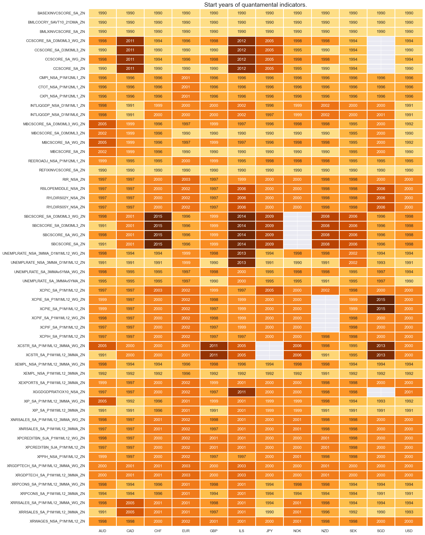
msm.check_availability(df, xcats=macroz, cids=cids_eq, missing_recent=False)

Conditional imputation of missing cross-sections

# Impute cross-sectional values if majority of cross sections are available

# Set parameters
impute_missing_cids = True
min_ratio_cids = 0.4

# Exclude categories than cannot logically be imputed
non_imputables = [
    "CXPI_NSA_P1M12ML1_ZN",
    "CMPI_NSA_P1M12ML1_ZN",
    "CTOT_NSA_P1M12ML1_ZN",
    "REEROADJ_NSA_P1M12ML1_ZN",
]
imputables = list(set(macroz) - set(non_imputables))

if impute_missing_cids:
    df_impute = msp.impute_panel(
        df=df, xcats=imputables, cids=cids_eq, threshold=min_ratio_cids
    )
    dfx = msm.update_df(df, df_impute)
else:
    dfx = df.copy()

# Visualize imputed macroeconomic categories
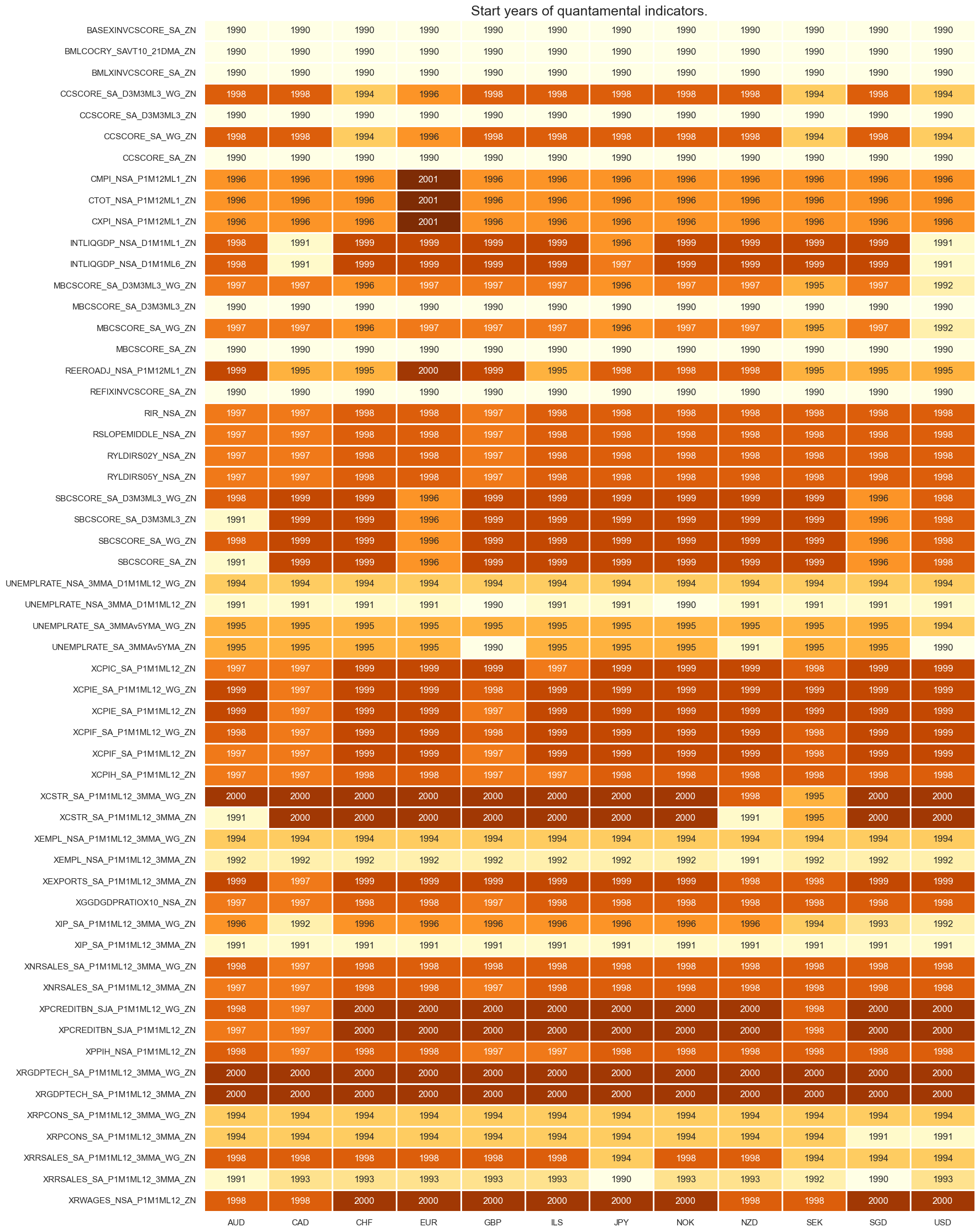
msm.check_availability(dfx, xcats=macroz, cids=cids_eq, missing_recent=False)

Equity sectoral return blacklisting

sector_blacklist = {}

for sec in list(set(cids_secs) - {"ALL"}):
    
    dfb = df[df["xcat"] == f"EQC{sec}UNTRADABLE_NSA"].loc[:, ["cid", "xcat", "real_date", "value"]]
    dfba = (
        dfb.groupby(["cid", "real_date"])
        .aggregate(value=pd.NamedAgg(column="value", aggfunc="max"))
        .reset_index()
    )
    dfba["xcat"] = f"EQC{sec}BLACK"
    
    sector_blacklist[sec] = msp.make_blacklist(dfba, f"EQC{sec}BLACK")

Visualize target availability

targets = [
    x for x in eqrets if x.endswith(("R_NSAvALL", "R_VT10vALL"))
]
msm.check_availability(dfx, targets, missing_recent=False)

Sectoral signals and naive PnLs

Common pipeline for all sectors

default_target_type = "R_VT10vALL"

Model hyperparameters

# Model dictionary
default_models = {
    "rf": RandomForestRegressor(
        n_estimators = 100,
        random_state = 42,
    )
}

# Hyperparameter grid   
default_hparam_grid = {
    "rf": {
        "max_samples": [0.1, 0.25],
        "max_features": ["sqrt", 0.5],
        "min_samples_leaf": [1, 3, 6, 9]
    },
}

Cross-validation splitter

default_splitter = {"Validation": msl.RecencyKFoldPanelSplit(n_periods=12, n_splits = 1)}

Validation metric

We use the probability of significance of correlation over the panel, arising from the MAP test, accounting for cross-sectional correlations in the panel, as a suitable performance metric. This should encourage the model selection process to favour models with evidence of predictive power, as well as capturing sufficient cross-sectional variation.

default_metric = {
    "MAP": make_scorer(msl.panel_significance_probability, greater_is_better=True),
}

Dynamics of the backtest

The initial training set is the smallest possible training set comprising two years’ of data for two cross-sections. This is specified by setting min_periods = 24 and min_cids = 2 . Model selection occurs each month, by specifying test_size = 1 . The start date of the backtest is January 2003, since the initial training set absorbs data.

# Default parameters
default_test_size = 1  # retraining interval in months
default_min_cids = 2  # minimum number of cids to start predicting
default_min_periods = 24  # minimum number of periods to start predicting
default_split_functions = None
default_start_date = "2003-01-31"  # start date for the analysis

Energy

Factor selection and signal generation

sector = "ENR"

enr_dict = {
    "sector_name": sector_labels[sector],
    "signal_name": f"{sector}SOL",
    "pnl_name": f"{sector_labels[sector]} learning-based signal",
    "xcatx": macroz,
    "cidx": list(set(cids_eq)-set(["CHF"])), # CHF has no energy companies
    "ret": f"EQC{sector}{default_target_type}",
    "freq": "M",
    "black": sector_blacklist[sector],
    "srr": None,
    "pnls": None,
}

xcatx = enr_dict["xcatx"] + [enr_dict["ret"]]
cidx = enr_dict["cidx"]

so_enr = msl.SignalOptimizer(
    df=dfx,
    xcats=xcatx,
    cids=cidx,
    blacklist=enr_dict["black"],
    freq=enr_dict["freq"],
    lag=1,
    xcat_aggs=["last", "sum"],
)

secname = enr_dict["sector_name"]
signal_name = enr_dict["signal_name"]

so_enr.calculate_predictions(
    name=signal_name,
    models=default_models,
    scorers=default_metric,
    hyperparameters=default_hparam_grid,
    inner_splitters=default_splitter,
    test_size=default_test_size,
    min_cids=default_min_cids,
    min_periods=default_min_periods,
    n_jobs_outer=-1,
    split_functions=default_split_functions,
)
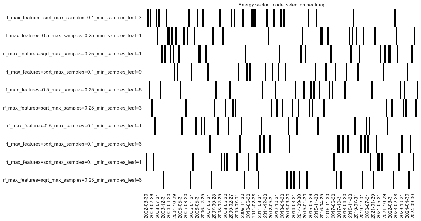
so_enr.models_heatmap(
    signal_name,
    cap=10,
    title=f"{secname} sector: model selection heatmap",
)

# Store signals
dfa = so_enr.get_optimized_signals()
dfx = msm.update_df(dfx, dfa)

enr_importances = (
    so_enr.feature_importances.describe()
    .iloc[:, 1:]
    .sort_values(by="mean", axis=1, ascending=False)
)

enr_importances

	BMLXINVCSCORE_SA_ZN	BMLCOCRY_SAVT10_21DMA_ZN	REFIXINVCSCORE_SA_ZN	BASEXINVCSCORE_SA_ZN	REEROADJ_NSA_P1M12ML1_ZN	RYLDIRS05Y_NSA_ZN	XPPIH_NSA_P1M1ML12_ZN	XRWAGES_NSA_P1M1ML12_ZN	XCSTR_SA_P1M1ML12_3MMA_WG_ZN	CCSCORE_SA_WG_ZN	...	UNEMPLRATE_NSA_3MMA_D1M1ML12_WG_ZN	CTOT_NSA_P1M12ML1_ZN	XEMPL_NSA_P1M1ML12_3MMA_ZN	MBCSCORE_SA_ZN	XRGDPTECH_SA_P1M1ML12_3MMA_WG_ZN	XIP_SA_P1M1ML12_3MMA_ZN	XEMPL_NSA_P1M1ML12_3MMA_WG_ZN	UNEMPLRATE_SA_3MMAv5YMA_WG_ZN	INTLIQGDP_NSA_D1M1ML6_ZN	INTLIQGDP_NSA_D1M1ML1_ZN
count	271.000000	271.000000	271.000000	271.000000	271.000000	271.000000	271.000000	271.000000	271.000000	271.000000	...	271.000000	271.000000	271.000000	271.000000	271.000000	271.000000	271.000000	271.000000	271.000000	271.000000
mean	0.030927	0.030094	0.024739	0.022718	0.021585	0.020675	0.020389	0.020245	0.019975	0.019587	...	0.015361	0.015102	0.015038	0.014972	0.014865	0.014725	0.014700	0.014543	0.013790	0.013005
min	0.000000	0.009212	0.004156	0.005009	0.011105	0.007890	0.008432	0.007092	0.002683	0.003043	...	0.002792	0.007286	0.000000	0.003520	0.004578	0.000388	0.006040	0.001652	0.003973	0.003130
25%	0.024789	0.025452	0.020337	0.019671	0.018761	0.017459	0.016626	0.017363	0.017500	0.016902	...	0.013154	0.013047	0.012971	0.012874	0.012466	0.012885	0.012704	0.012961	0.011421	0.011130
50%	0.029669	0.029542	0.024300	0.023108	0.021182	0.020781	0.019060	0.020288	0.019665	0.018822	...	0.015214	0.014534	0.015272	0.014778	0.014652	0.014541	0.014521	0.014691	0.013366	0.012912
75%	0.036705	0.034473	0.028142	0.026200	0.024050	0.023294	0.022669	0.022118	0.022515	0.022045	...	0.017299	0.016414	0.017252	0.016932	0.016736	0.016469	0.016623	0.016469	0.015574	0.014926
max	0.068146	0.065267	0.048316	0.045445	0.050443	0.055328	0.045022	0.041524	0.037962	0.040932	...	0.030651	0.040133	0.039301	0.035290	0.030890	0.027474	0.025039	0.025664	0.028522	0.022455
std	0.011594	0.007470	0.007346	0.005843	0.004575	0.005386	0.005957	0.004405	0.004936	0.004658	...	0.003907	0.003629	0.003765	0.003564	0.003489	0.003330	0.003006	0.003419	0.003595	0.003205

8 rows × 56 columns

xcatx = enr_dict["signal_name"]
secname = enr_dict["sector_name"]

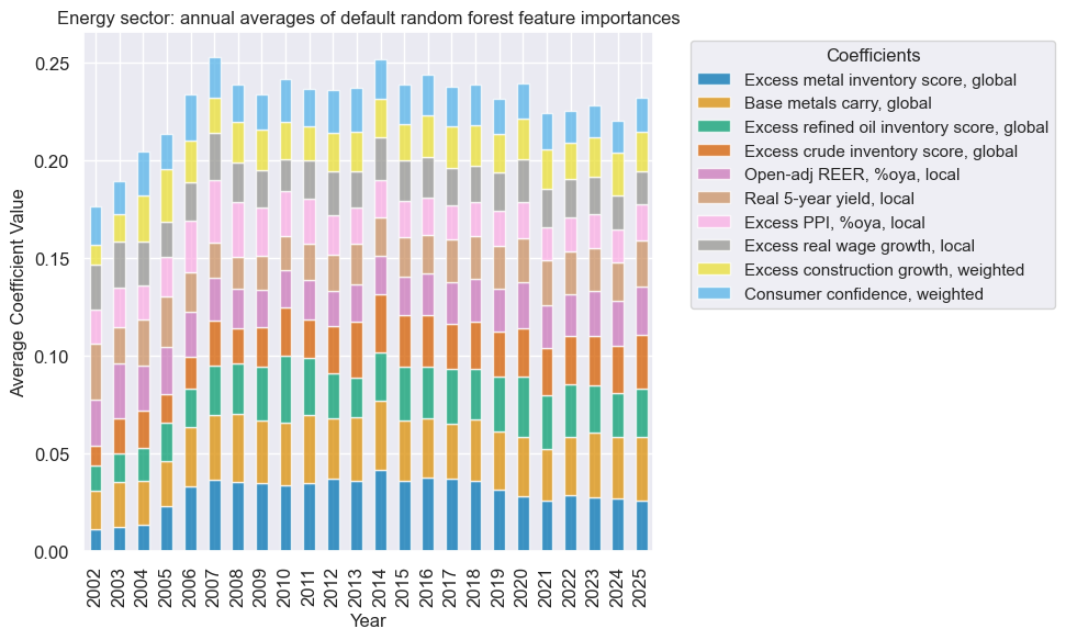
so_enr.coefs_stackedbarplot(
    name=xcatx,
    ftrs=list(enr_importances.columns[:10]),
    ftrs_renamed=cat_label_dict,
    title=f"{secname} sector: annual averages of default random forest feature importances",
)

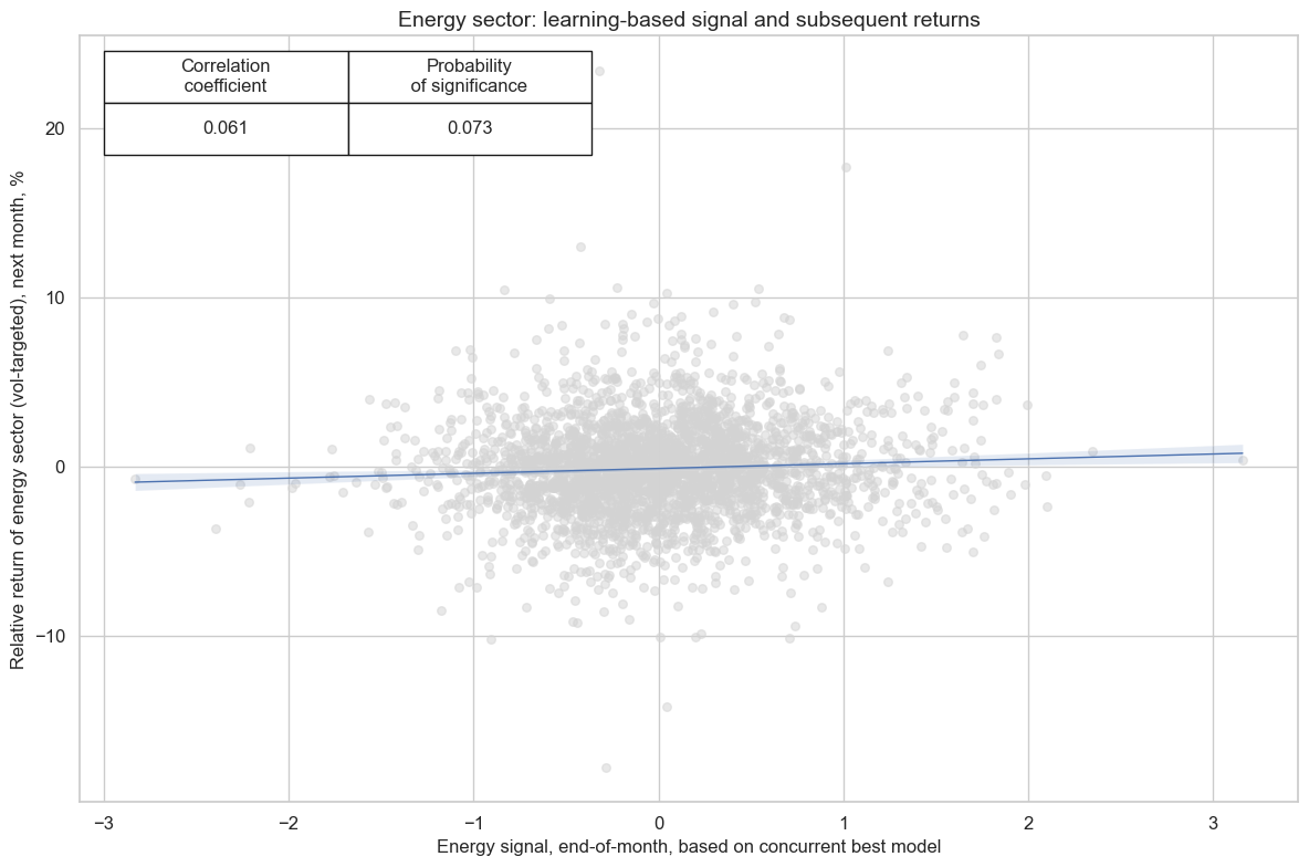
Signal quality check

xcatx = [enr_dict["signal_name"], enr_dict["ret"]]
cidx = enr_dict["cidx"]
secname = enr_dict["sector_name"]

cr_enr = msp.CategoryRelations(
    df=dfx,
    xcats=xcatx,
    cids=cidx,
    freq=enr_dict["freq"],
    lag=1,
    blacklist=enr_dict["black"],
    xcat_aggs=["last", "sum"],
    slip=1,
    xcat_trims=[30, 30],  # trim dodgy data point
)

cr_enr.reg_scatter(
    title=f"{secname} sector: learning-based signal and subsequent returns",
    labels=False,
    prob_est="map",
    xlab=f"{secname} signal, end-of-month, based on concurrent best model",
    ylab=f"Relative return of {secname.lower()} sector (vol-targeted), next month, %",
    coef_box="upper left",
    size=(12, 8),
)

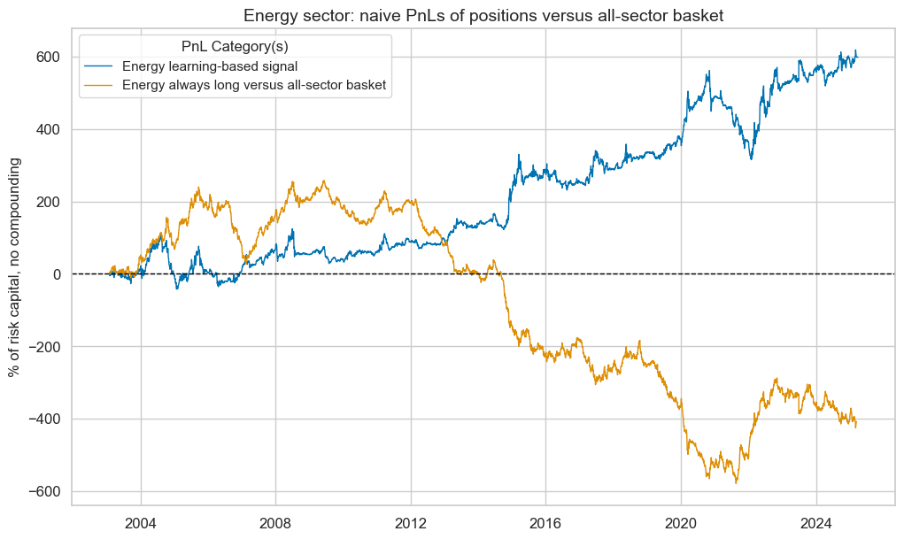
xcatx = [enr_dict["signal_name"]]
cidx = enr_dict["cidx"]
secname = enr_dict["sector_name"]

pnl_enr = msn.NaivePnL(
    df=dfx,
    ret=enr_dict["ret"],
    sigs=xcatx,
    cids=cidx,
    start=default_start_date,
    blacklist=enr_dict["black"],
    bms=["USD_EQXR_NSA"],
)

for xcat in xcatx:
    pnl_enr.make_pnl(
        sig=xcat,
        sig_op="zn_score_pan",
        rebal_freq="monthly",
        neutral="zero",
        rebal_slip=1,
        vol_scale=None,
        thresh=2,
        pnl_name=enr_dict["pnl_name"],
    )
pnl_enr.make_long_pnl(
    vol_scale=None, label=f"{secname} always long versus all-sector basket"
)

pnl_enr.plot_pnls(
    pnl_cats=pnl_enr.pnl_names,
    title=f"{secname} sector: naive PnLs of positions versus all-sector basket",
    title_fontsize=14,
)

enr_dict["pnls"] = pnl_enr
pnl_enr.evaluate_pnls(pnl_cats=pnl_enr.pnl_names)

xcat	Energy learning-based signal	Energy always long versus all-sector basket
Return %	27.019865	-18.469388
St. Dev. %	57.909781	53.016948
Sharpe Ratio	0.466586	-0.348368
Sortino Ratio	0.675189	-0.478872
Max 21-Day Draw %	-87.604987	-78.404808
Max 6-Month Draw %	-147.524394	-186.69396
Peak to Trough Draw %	-246.496899	-837.214078
Top 5% Monthly PnL Share	0.952336	-1.395043
USD_EQXR_NSA correl	-0.058604	-0.047811
Traded Months	267	267

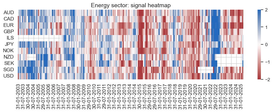
secname = enr_dict["sector_name"]

pnl_enr.signal_heatmap(
    pnl_name=enr_dict["pnl_name"],
    figsize=(12, 3),
    title=f"{secname} sector: signal heatmap",
)

Materials

Factor selection and signal generation

sector = "MAT"

mat_dict = {
    "sector_name": sector_labels[sector],
    "signal_name": f"{sector}SOL",
    "pnl_name": f"{sector_labels[sector]} learning-based signal",
    "xcatx": macroz,
    "cidx": cids_eq,
    "ret": f"EQC{sector}{default_target_type}",
    "freq": "M",
    "black": sector_blacklist[sector],
    "srr": None,
    "pnls": None,
}

xcatx = mat_dict["xcatx"] + [mat_dict["ret"]]
cidx = mat_dict["cidx"]

so_mat = msl.SignalOptimizer(
    df=dfx,
    xcats=xcatx,
    cids=cidx,
    blacklist=mat_dict["black"],
    freq=mat_dict["freq"],
    lag=1,
    xcat_aggs=["last", "sum"],
)

secname = mat_dict["sector_name"]
signal_name = mat_dict["signal_name"]

so_mat.calculate_predictions(
    name=signal_name,
    models=default_models,
    scorers=default_metric,
    hyperparameters=default_hparam_grid,
    inner_splitters=default_splitter,
    test_size=default_test_size,
    min_cids=default_min_cids,
    min_periods=default_min_periods,
    n_jobs_outer=-1,
    split_functions=default_split_functions,
)
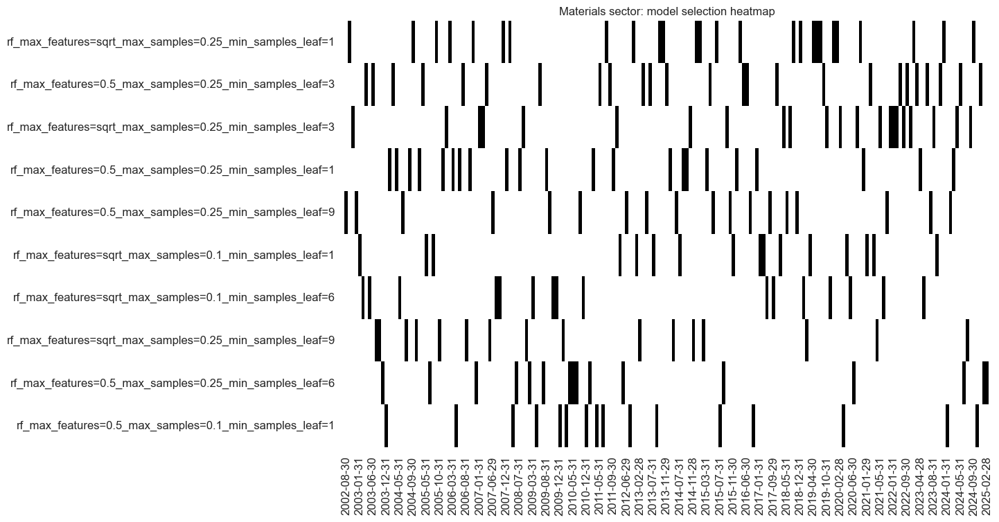
so_mat.models_heatmap(
    signal_name,
    cap=10,
    title=f"{secname} sector: model selection heatmap",
)

# Store signals
dfa = so_mat.get_optimized_signals()
dfx = msm.update_df(dfx, dfa)

mat_importances = (
    so_mat.feature_importances.describe()
    .iloc[:, 1:]
    .sort_values(by="mean", axis=1, ascending=False)
)

mat_importances

	REFIXINVCSCORE_SA_ZN	BMLCOCRY_SAVT10_21DMA_ZN	REEROADJ_NSA_P1M12ML1_ZN	SBCSCORE_SA_D3M3ML3_WG_ZN	CCSCORE_SA_WG_ZN	XCPIF_SA_P1M1ML12_WG_ZN	SBCSCORE_SA_D3M3ML3_ZN	RIR_NSA_ZN	BASEXINVCSCORE_SA_ZN	BMLXINVCSCORE_SA_ZN	...	RSLOPEMIDDLE_NSA_ZN	UNEMPLRATE_NSA_3MMA_D1M1ML12_WG_ZN	XCPIE_SA_P1M1ML12_ZN	MBCSCORE_SA_WG_ZN	XRGDPTECH_SA_P1M1ML12_3MMA_WG_ZN	MBCSCORE_SA_ZN	XRGDPTECH_SA_P1M1ML12_3MMA_ZN	XIP_SA_P1M1ML12_3MMA_ZN	INTLIQGDP_NSA_D1M1ML1_ZN	INTLIQGDP_NSA_D1M1ML6_ZN
count	271.000000	271.000000	271.000000	271.000000	271.000000	271.000000	271.000000	271.000000	271.000000	271.000000	...	271.000000	271.000000	271.000000	271.000000	271.000000	271.000000	271.000000	271.000000	271.000000	271.000000
mean	0.027414	0.027049	0.022460	0.022121	0.021919	0.021428	0.021095	0.020548	0.020401	0.020377	...	0.015399	0.015342	0.015168	0.015146	0.015032	0.014260	0.014090	0.013875	0.012206	0.011865
min	0.007395	0.014302	0.010688	0.006639	0.009518	0.009580	0.007751	0.008293	0.006952	0.001908	...	0.003000	0.007019	0.006584	0.004917	0.000000	0.004926	0.003038	0.002698	0.003795	0.004800
25%	0.023650	0.023519	0.019665	0.019426	0.019022	0.018857	0.018734	0.017751	0.017253	0.015761	...	0.013849	0.013341	0.013634	0.012960	0.013299	0.012679	0.011831	0.012321	0.010495	0.010215
50%	0.027418	0.026524	0.022170	0.021804	0.021169	0.020629	0.020799	0.020361	0.019915	0.020936	...	0.015407	0.014969	0.014956	0.014993	0.014808	0.014342	0.014043	0.013927	0.012253	0.011580
75%	0.030734	0.029970	0.024573	0.024508	0.023796	0.023231	0.023141	0.023172	0.023492	0.024669	...	0.016882	0.016645	0.016761	0.016988	0.016928	0.016275	0.015985	0.015305	0.014348	0.013206
max	0.043441	0.059587	0.041570	0.037830	0.038766	0.041611	0.034210	0.035389	0.041623	0.038614	...	0.028934	0.031476	0.031369	0.031679	0.027276	0.023415	0.025331	0.030235	0.019331	0.028560
std	0.006042	0.006272	0.004554	0.004668	0.004484	0.004530	0.004227	0.004572	0.005204	0.006792	...	0.002997	0.003495	0.002820	0.003364	0.003275	0.002851	0.003396	0.003003	0.002874	0.002573

8 rows × 56 columns

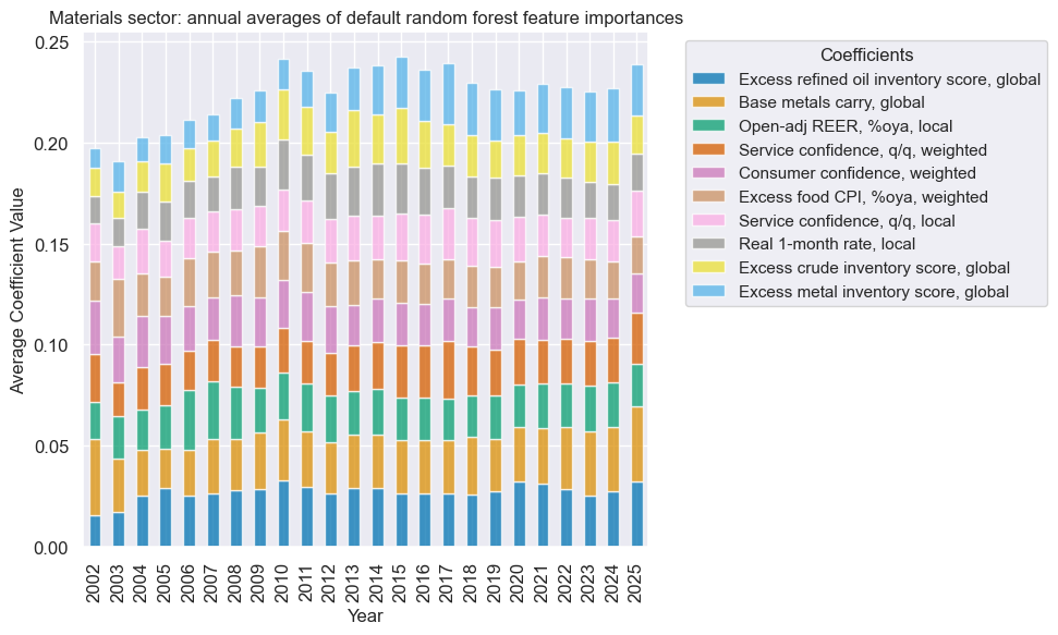
xcatx = mat_dict["signal_name"]
secname = mat_dict["sector_name"]

so_mat.coefs_stackedbarplot(
    name=xcatx,
    ftrs=list(mat_importances.columns[:10]),
    ftrs_renamed=cat_label_dict,
    title=f"{secname} sector: annual averages of default random forest feature importances",
)

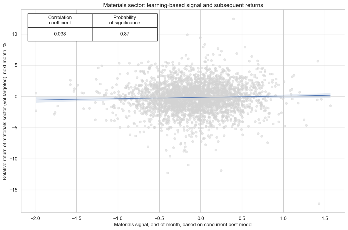
Signal quality check

xcatx = [mat_dict["signal_name"], mat_dict["ret"]]
cidx = mat_dict["cidx"]
secname = mat_dict["sector_name"]

cr_mat = msp.CategoryRelations(
    df=dfx,
    xcats=xcatx,
    cids=cidx,
    freq=mat_dict["freq"],
    blacklist=mat_dict["black"],
    lag=1,
    xcat_aggs=["last", "sum"],
    slip=1,
    xcat_trims=[2, 20],
)

cr_mat.reg_scatter(
    title=f"{secname} sector: learning-based signal and subsequent returns",
    labels=False,
    prob_est="map",
    xlab=f"{secname} signal, end-of-month, based on concurrent best model",
    ylab=f"Relative return of {secname.lower()} sector (vol-targeted), next month, %",
    coef_box="upper left",
    size=(12, 8),
)

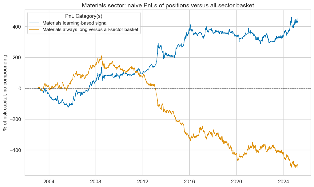
xcatx = [mat_dict["signal_name"]]
cidx = mat_dict["cidx"]
secname = mat_dict["sector_name"]
pnl_name = mat_dict["pnl_name"]

pnl_mat = msn.NaivePnL(
    df=dfx,
    ret=mat_dict["ret"],
    sigs=xcatx,
    cids=cidx,
    start=default_start_date,
    blacklist=mat_dict["black"],
    bms=["USD_EQXR_NSA"],
)

for xcat in xcatx:
    pnl_mat.make_pnl(
        sig=xcat,
        sig_op="zn_score_pan",
        rebal_freq="monthly",
        neutral="zero",
        rebal_slip=1,
        vol_scale=None,
        thresh=2,
        pnl_name=pnl_name,
    )
pnl_mat.make_long_pnl(
    vol_scale=None, label=f"{secname} always long versus all-sector basket"
)

pnl_mat.plot_pnls(
    pnl_cats=pnl_mat.pnl_names,
    title=f"{secname} sector: naive PnLs of positions versus all-sector basket",
    title_fontsize=14,
)

mat_dict["pnls"] = pnl_mat
pnl_mat.evaluate_pnls(pnl_cats=pnl_mat.pnl_names)

xcat	Materials learning-based signal	Materials always long versus all-sector basket
Return %	19.239838	-22.3526
St. Dev. %	43.681819	40.209911
Sharpe Ratio	0.440454	-0.555898
Sortino Ratio	0.619307	-0.76508
Max 21-Day Draw %	-74.894154	-61.657388
Max 6-Month Draw %	-92.416881	-152.838949
Peak to Trough Draw %	-127.270629	-725.96649
Top 5% Monthly PnL Share	1.175033	-0.718067
USD_EQXR_NSA correl	-0.015116	0.02638
Traded Months	267	267

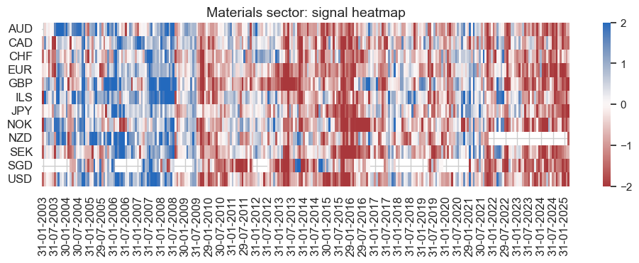
secname = mat_dict["sector_name"]
xcatx = mat_dict["signal_name"]

pnl_mat.signal_heatmap(
    pnl_name=f"{secname} learning-based signal",
    figsize=(12, 3),
    title=f"{secname} sector: signal heatmap",
)

Industrials

Factor selection and signal generation

sector = "IND"

ind_dict = {
    "sector_name": sector_labels[sector],
    "signal_name": f"{sector}SOL",
    "pnl_name": f"{sector_labels[sector]} learning-based signal",
    "xcatx": macroz,
    "cidx": cids_eq,
    "ret": f"EQC{sector}{default_target_type}",
    "freq": "M",
    "black": sector_blacklist[sector],
    "srr": None,
    "pnls": None,
}

xcatx = ind_dict["xcatx"] + [ind_dict["ret"]]
cidx = ind_dict["cidx"]

so_ind = msl.SignalOptimizer(
    df=dfx,
    xcats=xcatx,
    cids=cidx,
    blacklist=ind_dict["black"],
    freq=ind_dict["freq"],
    lag=1,
    xcat_aggs=["last", "sum"],
)

secname = ind_dict["sector_name"]
signal_name = ind_dict["signal_name"]

so_ind.calculate_predictions(
    name=signal_name,
    models=default_models,
    scorers=default_metric,
    hyperparameters=default_hparam_grid,
    inner_splitters=default_splitter,
    test_size=default_test_size,
    min_cids=default_min_cids,
    min_periods=default_min_periods,
    n_jobs_outer=-1,
    split_functions=default_split_functions,
)
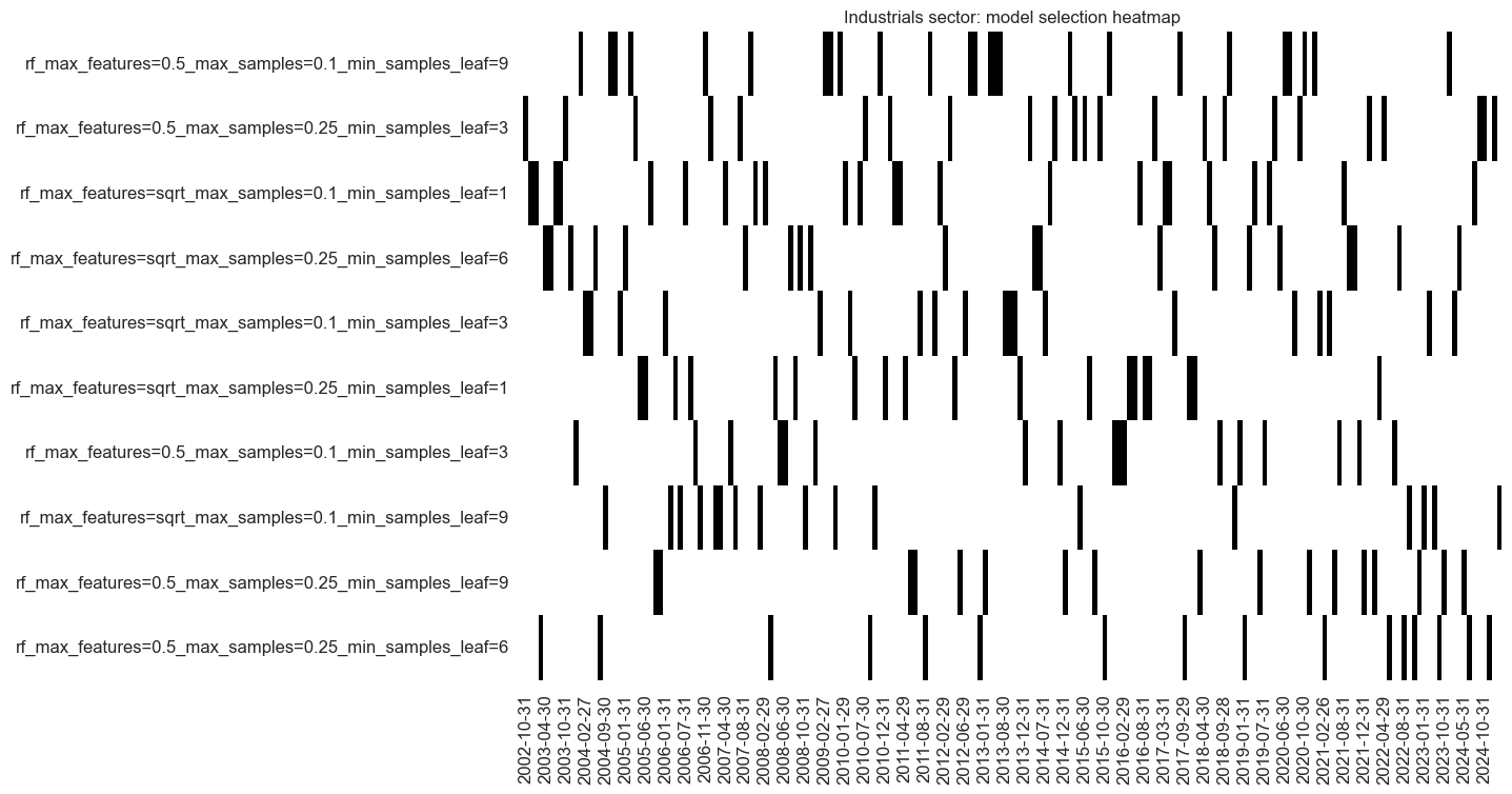
so_ind.models_heatmap(
    signal_name,
    cap=10,
    title=f"{secname} sector: model selection heatmap",
)

# Store signals
dfa = so_ind.get_optimized_signals()
dfx = msm.update_df(dfx, dfa)

ind_importances = (
    so_ind.feature_importances.describe()
    .iloc[:, 1:]
    .sort_values(by="mean", axis=1, ascending=False)
)

ind_importances

	BMLCOCRY_SAVT10_21DMA_ZN	BMLXINVCSCORE_SA_ZN	CCSCORE_SA_WG_ZN	XCPIC_SA_P1M1ML12_ZN	BASEXINVCSCORE_SA_ZN	XRWAGES_NSA_P1M1ML12_ZN	XGGDGDPRATIOX10_NSA_ZN	MBCSCORE_SA_D3M3ML3_ZN	XCPIE_SA_P1M1ML12_WG_ZN	REEROADJ_NSA_P1M12ML1_ZN	...	UNEMPLRATE_NSA_3MMA_D1M1ML12_ZN	XRGDPTECH_SA_P1M1ML12_3MMA_ZN	XRPCONS_SA_P1M1ML12_3MMA_WG_ZN	XEMPL_NSA_P1M1ML12_3MMA_WG_ZN	XIP_SA_P1M1ML12_3MMA_ZN	XRPCONS_SA_P1M1ML12_3MMA_ZN	XCPIH_SA_P1M1ML12_ZN	RIR_NSA_ZN	XEMPL_NSA_P1M1ML12_3MMA_ZN	INTLIQGDP_NSA_D1M1ML1_ZN
count	271.000000	271.000000	271.000000	271.000000	271.000000	271.000000	271.000000	271.000000	271.000000	271.000000	...	271.000000	271.000000	271.000000	271.000000	271.000000	271.000000	271.000000	271.000000	271.000000	271.000000
mean	0.035782	0.026190	0.021598	0.020993	0.020895	0.020396	0.020269	0.019732	0.019598	0.019488	...	0.015653	0.015401	0.015255	0.015094	0.015050	0.014864	0.014674	0.014487	0.014246	0.013209
min	0.001200	0.001582	0.008547	0.008321	0.001103	0.010902	0.005734	0.009563	0.000398	0.009110	...	0.001919	0.005062	0.005769	0.004008	0.002141	0.006500	0.000000	0.002947	0.004472	0.001726
25%	0.029026	0.021877	0.018609	0.018905	0.018042	0.017701	0.017809	0.017123	0.016979	0.017398	...	0.013528	0.013470	0.013813	0.013272	0.013410	0.013215	0.012972	0.012256	0.012710	0.011091
50%	0.033740	0.026367	0.020932	0.020921	0.021057	0.019834	0.020234	0.019195	0.019106	0.019147	...	0.015182	0.015275	0.015160	0.015190	0.015275	0.014849	0.014709	0.014735	0.014494	0.013062
75%	0.040701	0.031144	0.023798	0.023198	0.024177	0.021917	0.023116	0.021464	0.021519	0.021143	...	0.017085	0.017002	0.016606	0.016932	0.016577	0.016284	0.016159	0.016766	0.016095	0.014729
max	0.087346	0.048761	0.057077	0.034853	0.036690	0.045568	0.033274	0.038618	0.035167	0.036525	...	0.033791	0.025962	0.043339	0.027769	0.028080	0.023900	0.028253	0.025962	0.025550	0.032641
std	0.011091	0.008236	0.005121	0.003976	0.005166	0.004871	0.004086	0.004233	0.004670	0.003669	...	0.003430	0.002867	0.003433	0.003176	0.003307	0.002759	0.003117	0.003645	0.003023	0.003710

8 rows × 56 columns

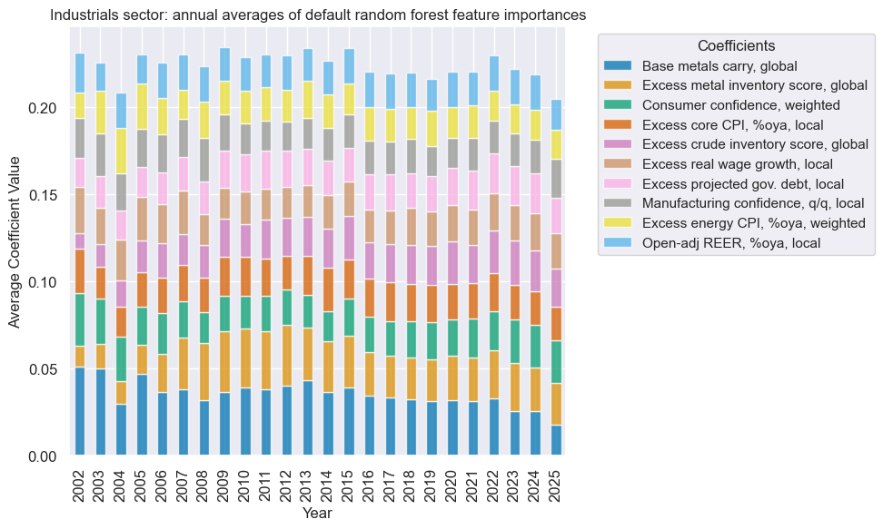
xcatx = ind_dict["signal_name"]
secname = ind_dict["sector_name"]

so_ind.coefs_stackedbarplot(
    name=xcatx,
    ftrs=list(ind_importances.columns[:10]),
    ftrs_renamed=cat_label_dict,
    title=f"{secname} sector: annual averages of default random forest feature importances",
)

Signal quality check

xcatx = [ind_dict["signal_name"], ind_dict["ret"]]
cidx = ind_dict["cidx"]
secname = ind_dict["sector_name"]

cr_ind = msp.CategoryRelations(
    df=dfx,
    xcats=xcatx,
    cids=cidx,
    freq=ind_dict["freq"],
    blacklist=ind_dict["black"],
    lag=1,
    xcat_aggs=["last", "sum"],
    slip=1,
)

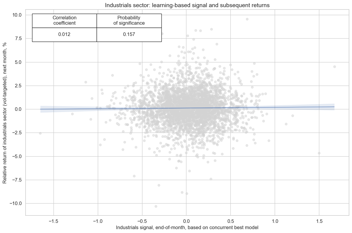
cr_ind.reg_scatter(
    title=f"{secname} sector: learning-based signal and subsequent returns",
    labels=False,
    prob_est="map",
    xlab=f"{secname} signal, end-of-month, based on concurrent best model",
    ylab=f"Relative return of {secname.lower()} sector (vol-targeted), next month, %",
    coef_box="upper left",
    size=(12, 8),
)

xcatx = [ind_dict["signal_name"]]
cidx = ind_dict["cidx"]
secname = ind_dict["sector_name"]
pnl_name = ind_dict["pnl_name"]

pnl_ind = msn.NaivePnL(
    df=dfx,
    ret=ind_dict["ret"],
    sigs=xcatx,
    cids=cidx,
    start=default_start_date,
    bms=["USD_EQXR_NSA"],
    blacklist=ind_dict["black"],
)

for xcat in xcatx:
    pnl_ind.make_pnl(
        sig=xcat,
        sig_op="zn_score_pan",
        rebal_freq="monthly",
        neutral="zero",
        rebal_slip=1,
        vol_scale=None,
        thresh=2,
        pnl_name=pnl_name,
    )

    pnl_ind.make_long_pnl(
        vol_scale=None, label=f"{secname} always long versus all-sector basket"
    )

pnl_ind.plot_pnls(
    pnl_cats=pnl_ind.pnl_names,
    title=f"{secname} sector: naive PnLs of positions versus all-sector basket",
    title_fontsize=14,
)

ind_dict["pnls"] = pnl_ind
pnl_ind.evaluate_pnls(pnl_cats=pnl_ind.pnl_names)

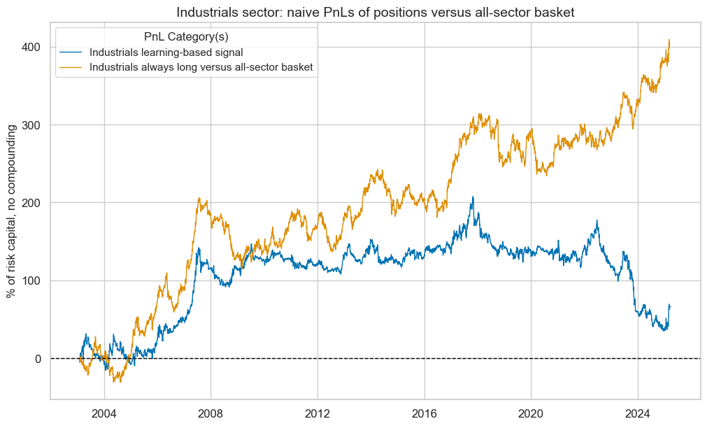
xcat	Industrials learning-based signal	Industrials always long versus all-sector basket
Return %	2.99681	18.300281
St. Dev. %	27.296944	31.947543
Sharpe Ratio	0.109786	0.572823
Sortino Ratio	0.155486	0.819209
Max 21-Day Draw %	-35.858828	-54.172009
Max 6-Month Draw %	-77.279286	-63.203195
Peak to Trough Draw %	-172.77989	-91.886853
Top 5% Monthly PnL Share	3.59211	0.794551
USD_EQXR_NSA correl	-0.001896	0.263312
Traded Months	267	267

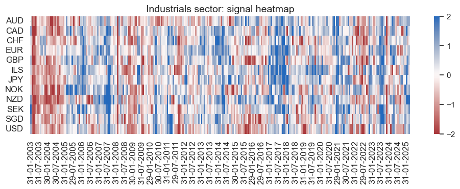
xcatx = ind_dict["signal_name"]
pnl_ind.signal_heatmap(
    pnl_name=f"{secname} learning-based signal",
    figsize=(12, 3),
    title=f"{secname} sector: signal heatmap",
)

Consumer discretionary

Factor selection and signal generation

sector = "COD"

cod_dict = {
    "sector_name": sector_labels[sector],
    "signal_name": f"{sector}SOL",
    "pnl_name": f"{sector_labels[sector]} learning-based signal",
    "xcatx": macroz,
    "cidx": cids_eq,
    "ret": f"EQC{sector}{default_target_type}",
    "freq": "M",
    "black": sector_blacklist[sector],
    "srr": None,
    "pnls": None,
}

xcatx = cod_dict["xcatx"] + [cod_dict["ret"]]
cidx = cod_dict["cidx"]

so_cod = msl.SignalOptimizer(
    df=dfx,
    xcats=xcatx,
    cids=cidx,
    blacklist=cod_dict["black"],
    freq=cod_dict["freq"],
    lag=1,
    xcat_aggs=["last", "sum"],
)

secname = cod_dict["sector_name"]
signal_name = cod_dict["signal_name"]

so_cod.calculate_predictions(
    name=signal_name,
    models=default_models,
    scorers=default_metric,
    hyperparameters=default_hparam_grid,
    inner_splitters=default_splitter,
    test_size=default_test_size,
    min_cids=default_min_cids,
    min_periods=default_min_periods,
    n_jobs_outer=-1,
    split_functions=default_split_functions,
)
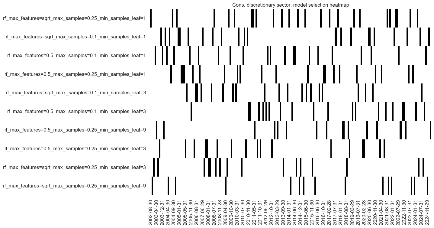
so_cod.models_heatmap(
    signal_name,
    cap=10,
    title=f"{secname} sector: model selection heatmap",
)

# Store signals
dfa = so_cod.get_optimized_signals()
dfx = msm.update_df(dfx, dfa)

cod_importances = (
    so_cod.feature_importances.describe()
    .iloc[:, 1:]
    .sort_values(by="mean", axis=1, ascending=False)
)

cod_importances

	XGGDGDPRATIOX10_NSA_ZN	BMLCOCRY_SAVT10_21DMA_ZN	CXPI_NSA_P1M12ML1_ZN	SBCSCORE_SA_WG_ZN	XRWAGES_NSA_P1M1ML12_ZN	REEROADJ_NSA_P1M12ML1_ZN	REFIXINVCSCORE_SA_ZN	RYLDIRS05Y_NSA_ZN	RYLDIRS02Y_NSA_ZN	XCSTR_SA_P1M1ML12_3MMA_ZN	...	XIP_SA_P1M1ML12_3MMA_ZN	CMPI_NSA_P1M12ML1_ZN	XRRSALES_SA_P1M1ML12_3MMA_WG_ZN	XRPCONS_SA_P1M1ML12_3MMA_ZN	XEMPL_NSA_P1M1ML12_3MMA_ZN	MBCSCORE_SA_WG_ZN	XRGDPTECH_SA_P1M1ML12_3MMA_ZN	INTLIQGDP_NSA_D1M1ML6_ZN	XPCREDITBN_SJA_P1M1ML12_WG_ZN	INTLIQGDP_NSA_D1M1ML1_ZN
count	271.000000	271.000000	271.000000	271.000000	271.000000	271.000000	271.000000	271.000000	271.000000	271.000000	...	271.000000	271.000000	271.000000	271.000000	271.000000	271.000000	271.000000	271.000000	271.000000	271.000000
mean	0.023720	0.022884	0.021065	0.020744	0.020660	0.020552	0.020328	0.020307	0.020209	0.020147	...	0.016136	0.016098	0.016097	0.015706	0.015676	0.015588	0.015326	0.014716	0.014528	0.013099
min	0.005425	0.004415	0.012036	0.002538	0.009775	0.008190	0.008505	0.008254	0.010714	0.008822	...	0.009056	0.006869	0.000000	0.006480	0.000000	0.002798	0.008000	0.005364	0.002427	0.004376
25%	0.020339	0.020078	0.018426	0.018718	0.018207	0.018561	0.017812	0.017741	0.017637	0.017676	...	0.014114	0.013944	0.014115	0.014244	0.013938	0.013636	0.013681	0.012040	0.012425	0.011148
50%	0.023477	0.022541	0.020640	0.020686	0.020199	0.020335	0.020242	0.020563	0.019872	0.019740	...	0.016033	0.015886	0.015470	0.015748	0.015579	0.015842	0.015222	0.013599	0.014420	0.013183
75%	0.026788	0.025686	0.022816	0.022753	0.022655	0.022469	0.022743	0.022598	0.022159	0.021900	...	0.017760	0.018247	0.017740	0.017207	0.018010	0.017568	0.016969	0.015767	0.016280	0.014892
max	0.043029	0.042228	0.038962	0.031806	0.044011	0.036594	0.035118	0.034091	0.055859	0.036420	...	0.043016	0.025852	0.040442	0.024967	0.032890	0.028128	0.026256	0.035685	0.030991	0.028887
std	0.005174	0.005089	0.004082	0.004021	0.004167	0.003641	0.004283	0.004323	0.004684	0.004086	...	0.003433	0.003143	0.003898	0.002873	0.003687	0.003406	0.002775	0.004601	0.003149	0.003064

8 rows × 56 columns

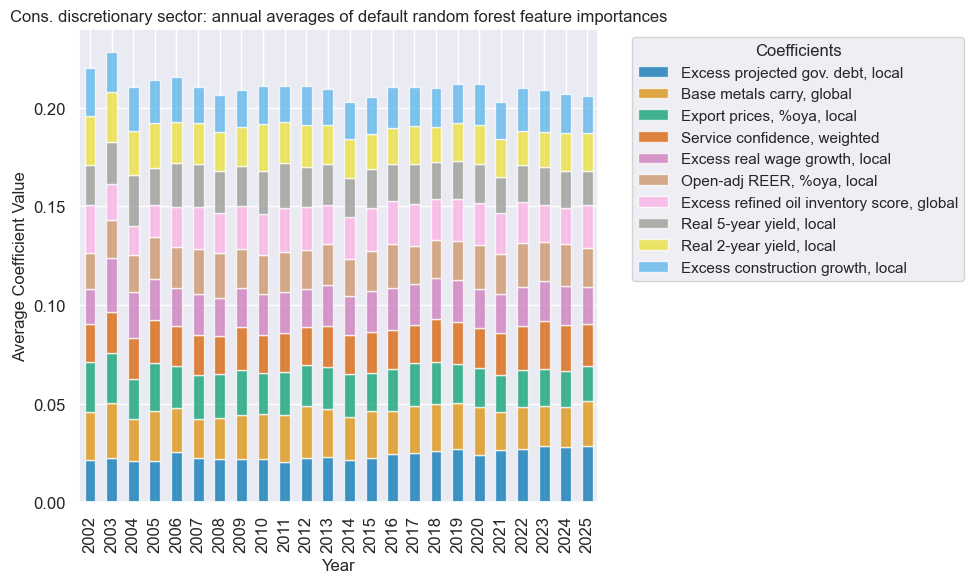
xcatx = cod_dict["signal_name"]
secname = cod_dict["sector_name"]

so_cod.coefs_stackedbarplot(
    name=xcatx,
    ftrs=list(cod_importances.columns[:10]),
    ftrs_renamed=cat_label_dict,
    title=f"{secname} sector: annual averages of default random forest feature importances",
)

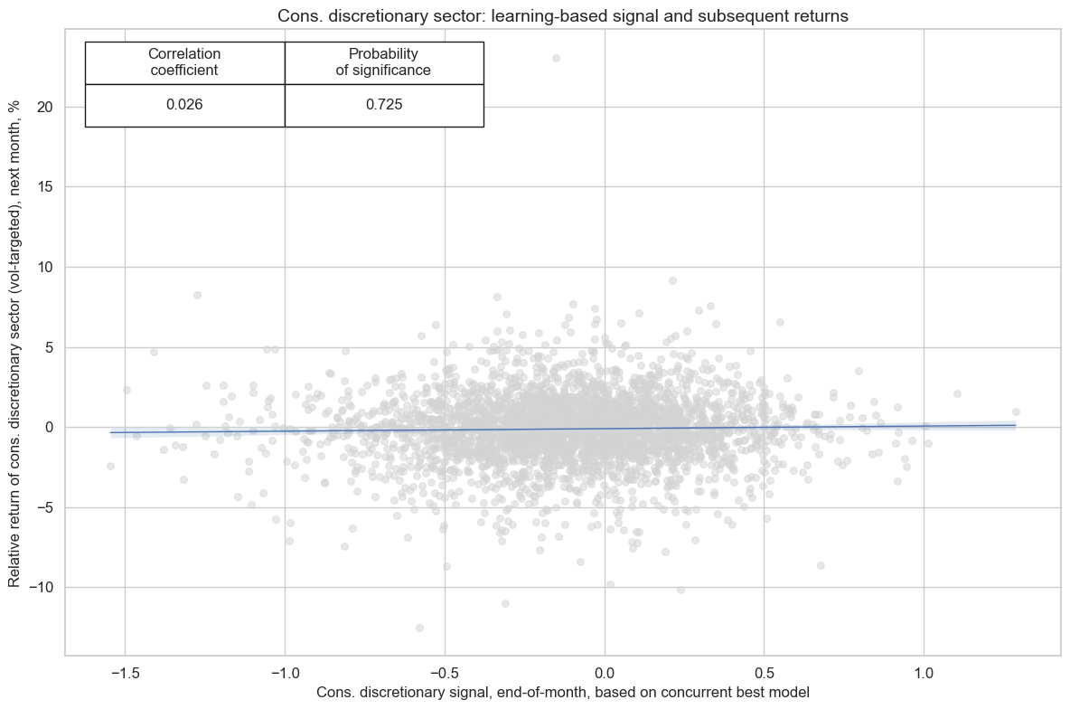
Signal quality check

xcatx = [cod_dict["signal_name"], cod_dict["ret"]]
cidx = cod_dict["cidx"]
signal_name = cod_dict["signal_name"]

cr_cod = msp.CategoryRelations(
    df=dfx,
    xcats=xcatx,
    cids=cidx,
    freq=cod_dict["freq"],
    blacklist=cod_dict["black"],
    lag=1,
    xcat_aggs=["last", "sum"],
    slip=1,
)

cr_cod.reg_scatter(
    title=f"{secname} sector: learning-based signal and subsequent returns",
    labels=False,
    prob_est="map",
    xlab=f"{secname} signal, end-of-month, based on concurrent best model",
    ylab=f"Relative return of {secname.lower()} sector (vol-targeted), next month, %",
    coef_box="upper left",
    size=(12, 8),
)

xcatx = [cod_dict["signal_name"]]
cidx = cod_dict["cidx"]
secname = cod_dict["sector_name"]
signal_name = cod_dict["signal_name"]
pnl_name = cod_dict["pnl_name"]

pnl_cod = msn.NaivePnL(
    df=dfx,
    ret=cod_dict["ret"],
    sigs=xcatx,
    cids=cidx,
    start=default_start_date,
    blacklist=cod_dict["black"],
    bms=["USD_EQXR_NSA"],
)

for xcat in xcatx:
    pnl_cod.make_pnl(
        sig=xcat,
        sig_op="zn_score_pan",
        rebal_freq="monthly",
        neutral="zero",
        rebal_slip=1,
        vol_scale=None,
        thresh=2,
        pnl_name=pnl_name,
    )
pnl_cod.make_long_pnl(
    vol_scale=None, label=f"{secname} always long versus all-sector basket"
)

pnl_cod.plot_pnls(
    pnl_cats=pnl_cod.pnl_names,
    title=f"{secname} sector: naive PnLs of positions versus all-sector basket",
    title_fontsize=14,
)

cod_dict["pnls"] = pnl_cod
pnl_cod.evaluate_pnls(pnl_cats=pnl_cod.pnl_names)

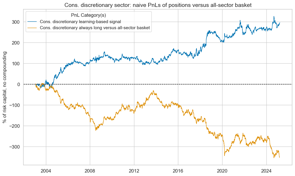
xcat	Cons. discretionary learning-based signal	Cons. discretionary always long versus all-sector basket
Return %	13.310832	-15.978518
St. Dev. %	31.809486	31.322219
Sharpe Ratio	0.418455	-0.510134
Sortino Ratio	0.611507	-0.705453
Max 21-Day Draw %	-36.940937	-68.480798
Max 6-Month Draw %	-58.975361	-96.360886
Peak to Trough Draw %	-70.278802	-358.531109
Top 5% Monthly PnL Share	1.04814	-0.737259
USD_EQXR_NSA correl	-0.006917	0.095431
Traded Months	267	267

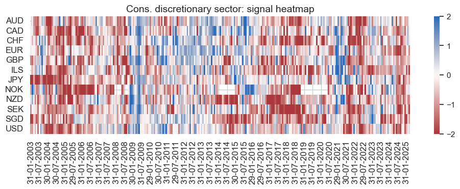
pnl_name = cod_dict["pnl_name"]
secname = cod_dict["sector_name"]

pnl_cod.signal_heatmap(
    pnl_name=f"{secname} learning-based signal",
    figsize=(12, 3),
    title=f"{secname} sector: signal heatmap",
)

Consumer staples

Factor selection and signal generation

sector = "COS"

cos_dict = {
    "sector_name": sector_labels[sector],
    "signal_name": f"{sector}SOL",
    "pnl_name": f"{sector_labels[sector]} learning-based signal",
    "xcatx": macroz,
    "cidx": cids_eq,
    "ret": f"EQC{sector}{default_target_type}",
    "freq": "M",
    "black": sector_blacklist[sector],
    "srr": None,
    "pnls": None,
}

xcatx = cos_dict["xcatx"] + [cos_dict["ret"]]
cidx = cos_dict["cidx"]

so_cos = msl.SignalOptimizer(
    df=dfx,
    xcats=xcatx,
    cids=cidx,
    blacklist=cos_dict["black"],
    freq=cos_dict["freq"],
    lag=1,
    xcat_aggs=["last", "sum"],
)

secname = cos_dict["sector_name"]
signal_name = cos_dict["signal_name"]

so_cos.calculate_predictions(
    name=signal_name,
    models=default_models,
    scorers=default_metric,
    hyperparameters=default_hparam_grid,
    inner_splitters=default_splitter,
    test_size=default_test_size,
    min_cids=default_min_cids,
    min_periods=default_min_periods,
    n_jobs_outer=-1,
    split_functions=default_split_functions,
)
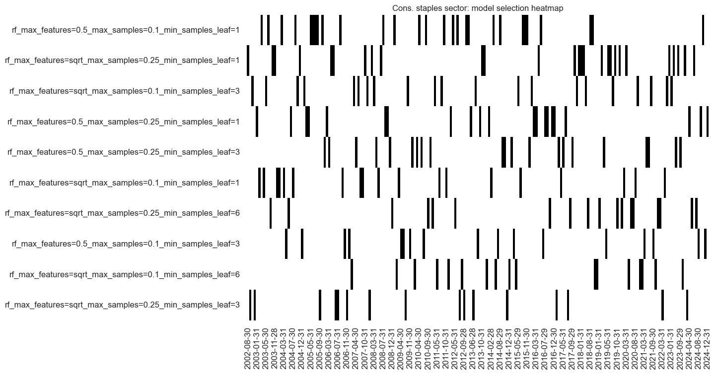
so_cos.models_heatmap(
    signal_name,
    cap=10,
    title=f"{secname} sector: model selection heatmap",
)

# Store signals
dfa = so_cos.get_optimized_signals()
dfx = msm.update_df(dfx, dfa)

cos_importances = (
    so_cos.feature_importances.describe()
    .iloc[:, 1:]
    .sort_values(by="mean", axis=1, ascending=False)
)

cos_importances

	BMLCOCRY_SAVT10_21DMA_ZN	CCSCORE_SA_WG_ZN	REEROADJ_NSA_P1M12ML1_ZN	XCPIF_SA_P1M1ML12_WG_ZN	XGGDGDPRATIOX10_NSA_ZN	RYLDIRS02Y_NSA_ZN	RYLDIRS05Y_NSA_ZN	XIP_SA_P1M1ML12_3MMA_WG_ZN	XRGDPTECH_SA_P1M1ML12_3MMA_WG_ZN	SBCSCORE_SA_D3M3ML3_WG_ZN	...	UNEMPLRATE_NSA_3MMA_D1M1ML12_WG_ZN	INTLIQGDP_NSA_D1M1ML6_ZN	XRPCONS_SA_P1M1ML12_3MMA_ZN	XPPIH_NSA_P1M1ML12_ZN	XEMPL_NSA_P1M1ML12_3MMA_ZN	XRPCONS_SA_P1M1ML12_3MMA_WG_ZN	MBCSCORE_SA_WG_ZN	MBCSCORE_SA_ZN	CMPI_NSA_P1M12ML1_ZN	INTLIQGDP_NSA_D1M1ML1_ZN
count	271.000000	271.000000	271.000000	271.000000	271.000000	271.000000	271.000000	271.000000	271.000000	271.000000	...	271.000000	271.000000	271.000000	271.000000	271.000000	271.000000	271.000000	271.000000	271.000000	271.000000
mean	0.030157	0.024069	0.023923	0.022014	0.020905	0.020691	0.020386	0.019763	0.019729	0.018906	...	0.016139	0.016108	0.016090	0.016060	0.015942	0.015932	0.015433	0.015346	0.014584	0.014198
min	0.013596	0.015575	0.014411	0.011093	0.003462	0.009548	0.011545	0.011905	0.008197	0.008619	...	0.008253	0.009533	0.007149	0.007429	0.006567	0.008011	0.006665	0.006510	0.006187	0.004975
25%	0.025807	0.020668	0.021228	0.018115	0.017665	0.016654	0.018259	0.016571	0.015770	0.016757	...	0.013540	0.013454	0.014459	0.014369	0.014403	0.013922	0.013399	0.013700	0.012842	0.012064
50%	0.029968	0.022965	0.023401	0.020101	0.021223	0.020174	0.020438	0.018308	0.017930	0.019150	...	0.015510	0.015275	0.016031	0.016081	0.016171	0.015534	0.015764	0.015556	0.014787	0.014135
75%	0.034097	0.026491	0.026160	0.024199	0.024560	0.024059	0.022173	0.021438	0.021581	0.021054	...	0.018204	0.018512	0.017752	0.017601	0.017659	0.017627	0.017429	0.017042	0.016022	0.015899
max	0.049511	0.044102	0.052365	0.065414	0.038626	0.042761	0.040571	0.045291	0.062926	0.029366	...	0.035063	0.026862	0.028448	0.031605	0.024552	0.028617	0.022328	0.026688	0.024257	0.024153
std	0.006278	0.005038	0.004585	0.006757	0.005430	0.005823	0.003647	0.005054	0.006634	0.003355	...	0.003841	0.003531	0.002808	0.002854	0.002888	0.003207	0.002820	0.002978	0.002672	0.003033

8 rows × 56 columns

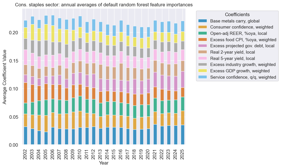
xcatx = cos_dict["signal_name"]
secname = cos_dict["sector_name"]

so_cos.coefs_stackedbarplot(
    name=xcatx,
    ftrs=list(cos_importances.columns[:10]),
    ftrs_renamed=cat_label_dict,
    title=f"{secname} sector: annual averages of default random forest feature importances",
)

Signal quality check

xcatx = [cos_dict["signal_name"], cos_dict["ret"]]
cidx = cos_dict["cidx"]
secname = cos_dict["sector_name"]

cr_cos = msp.CategoryRelations(
    df=dfx,
    xcats=xcatx,
    cids=cidx,
    freq=cos_dict["freq"],
    blacklist=cos_dict["black"],
    lag=1,
    xcat_aggs=["last", "sum"],
    slip=1,
)

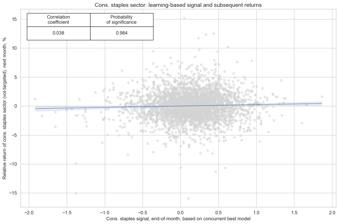
cr_cos.reg_scatter(
    title=f"{secname} sector: learning-based signal and subsequent returns",
    labels=False,
    prob_est="map",
    xlab=f"{secname} signal, end-of-month, based on concurrent best model",
    ylab=f"Relative return of {secname.lower()} sector (vol-targeted), next month, %",
    coef_box="upper left",
    size=(12, 8),
)

xcatx = [cos_dict["signal_name"]]
cidx = cos_dict["cidx"]
secname = cos_dict["sector_name"]
signal_name = cos_dict["signal_name"]
pnl_name = cos_dict["pnl_name"]

pnl_cos = msn.NaivePnL(
    df=dfx,
    ret=cos_dict["ret"],
    sigs=xcatx,
    cids=cidx,
    start=default_start_date,
    blacklist=cos_dict["black"],
    bms=["USD_EQXR_NSA"],
)

for xcat in xcatx:
    pnl_cos.make_pnl(
        sig=xcat,
        sig_op="zn_score_pan",
        rebal_freq="monthly",
        neutral="zero",
        rebal_slip=1,
        vol_scale=None,
        thresh=2,
        pnl_name=pnl_name,
    )
pnl_cos.make_long_pnl(
    vol_scale=None, label=f"{secname} always long versus all-sector basket"
)

pnl_cos.plot_pnls(
    pnl_cats=pnl_cos.pnl_names,
    title=f"{secname} sector: naive PnLs of positions versus all-sector basket",
    title_fontsize=14,
)

cos_dict["pnls"] = pnl_cos
pnl_cos.evaluate_pnls(pnl_cats=pnl_cos.pnl_names)

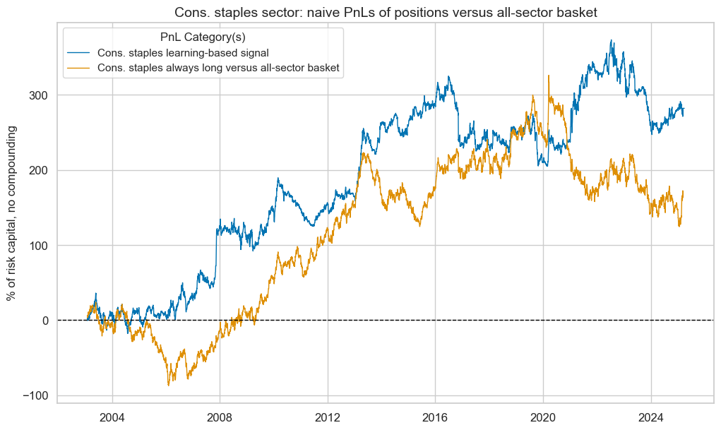
xcat	Cons. staples learning-based signal	Cons. staples always long versus all-sector basket
Return %	12.729819	7.386778
St. Dev. %	37.829007	37.762289
Sharpe Ratio	0.336509	0.195613
Sortino Ratio	0.478747	0.281357
Max 21-Day Draw %	-52.720556	-33.681565
Max 6-Month Draw %	-90.375119	-93.828486
Peak to Trough Draw %	-126.18286	-201.569822
Top 5% Monthly PnL Share	1.438746	2.354328
USD_EQXR_NSA correl	-0.064439	-0.138678
Traded Months	267	267

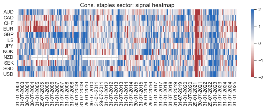
pnl_name = cos_dict["pnl_name"]
secname = cos_dict["sector_name"]

pnl_cos.signal_heatmap(
    pnl_name=pnl_name,
    figsize=(12, 3),
    title=f"{secname} sector: signal heatmap",
)

Healthcare

Factor selection and signal generation

sector = "HLC"

hlc_dict = {
    "sector_name": sector_labels[sector],
    "signal_name": f"{sector}SOL",
    "pnl_name": f"{sector_labels[sector]} learning-based signal",
    "xcatx": macroz,
    "cidx": cids_eq,
    "ret": f"EQC{sector}{default_target_type}",
    "freq": "M",
    "black": sector_blacklist[sector],
    "srr": None,
    "pnls": None,
}

xcatx = hlc_dict["xcatx"] + [hlc_dict["ret"]]
cidx = hlc_dict["cidx"]

so_hlc = msl.SignalOptimizer(
    df=dfx,
    xcats=xcatx,
    cids=cidx,
    blacklist=hlc_dict["black"],
    freq=hlc_dict["freq"],
    lag=1,
    xcat_aggs=["last", "sum"],
)

secname = hlc_dict["sector_name"]
signal_name = hlc_dict["signal_name"]

so_hlc.calculate_predictions(
    name=signal_name,
    models=default_models,
    scorers=default_metric,
    hyperparameters=default_hparam_grid,
    inner_splitters=default_splitter,
    test_size=default_test_size,
    min_cids=default_min_cids,
    min_periods=default_min_periods,
    n_jobs_outer=-1,
    split_functions=default_split_functions,
)
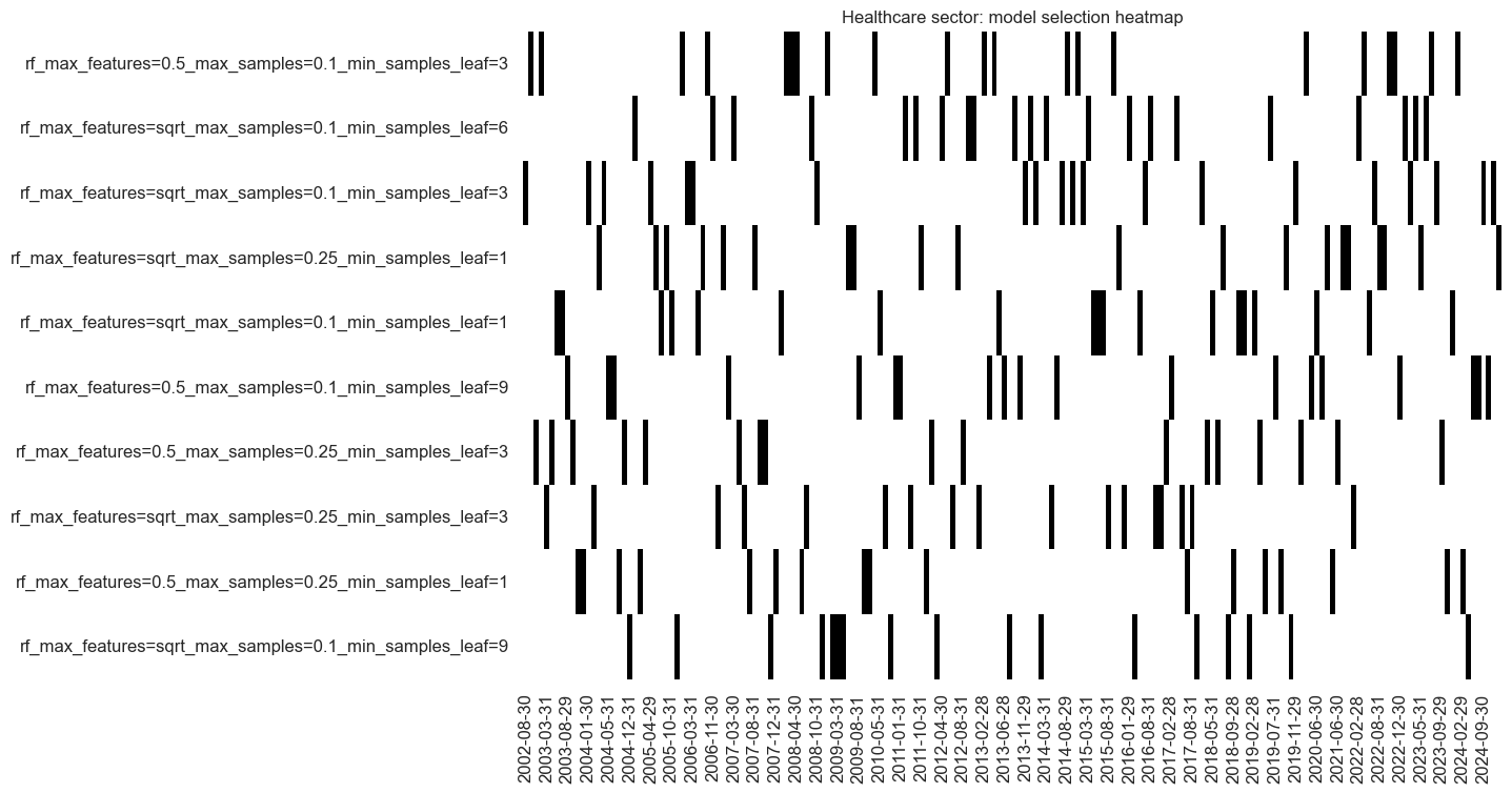
so_hlc.models_heatmap(
    signal_name,
    cap=10,
    title=f"{secname} sector: model selection heatmap",
)

# Store signals
dfa = so_hlc.get_optimized_signals()
dfx = msm.update_df(dfx, dfa)

hlc_importances = (
    so_hlc.feature_importances.describe()
    .iloc[:, 1:]
    .sort_values(by="mean", axis=1, ascending=False)
)

hlc_importances

	BMLCOCRY_SAVT10_21DMA_ZN	XRWAGES_NSA_P1M1ML12_ZN	REFIXINVCSCORE_SA_ZN	XCPIC_SA_P1M1ML12_ZN	XGGDGDPRATIOX10_NSA_ZN	BMLXINVCSCORE_SA_ZN	REEROADJ_NSA_P1M12ML1_ZN	XCPIF_SA_P1M1ML12_WG_ZN	INTLIQGDP_NSA_D1M1ML6_ZN	XCSTR_SA_P1M1ML12_3MMA_ZN	...	XPCREDITBN_SJA_P1M1ML12_WG_ZN	XRGDPTECH_SA_P1M1ML12_3MMA_ZN	XEMPL_NSA_P1M1ML12_3MMA_ZN	UNEMPLRATE_NSA_3MMA_D1M1ML12_WG_ZN	UNEMPLRATE_SA_3MMAv5YMA_WG_ZN	XEMPL_NSA_P1M1ML12_3MMA_WG_ZN	XIP_SA_P1M1ML12_3MMA_ZN	RYLDIRS02Y_NSA_ZN	XRGDPTECH_SA_P1M1ML12_3MMA_WG_ZN	INTLIQGDP_NSA_D1M1ML1_ZN
count	271.000000	271.000000	271.000000	271.000000	271.000000	271.000000	271.000000	271.000000	271.000000	271.000000	...	271.000000	271.000000	271.000000	271.000000	271.000000	271.000000	271.000000	271.000000	271.000000	271.000000
mean	0.028836	0.022154	0.021328	0.021144	0.021050	0.019896	0.019867	0.019775	0.019761	0.019534	...	0.015664	0.015538	0.015405	0.015398	0.015327	0.015251	0.015046	0.015034	0.014766	0.012400
min	0.010444	0.011627	0.000000	0.001824	0.005830	0.005647	0.006950	0.010341	0.006135	0.010893	...	0.004780	0.003910	0.003051	0.004595	0.002467	0.006907	0.007852	0.002245	0.005999	0.000000
25%	0.023714	0.019355	0.017098	0.018512	0.018416	0.016864	0.017720	0.017549	0.014760	0.017126	...	0.013829	0.013552	0.013630	0.013150	0.013432	0.013427	0.013374	0.012737	0.013133	0.010878
50%	0.026868	0.021686	0.021552	0.020574	0.020974	0.020205	0.019845	0.019464	0.017453	0.019279	...	0.015973	0.015623	0.015585	0.014772	0.015331	0.015048	0.015252	0.015094	0.014687	0.012463
75%	0.031702	0.023954	0.024864	0.023787	0.023622	0.023262	0.021969	0.021538	0.023129	0.021409	...	0.017566	0.017730	0.017440	0.017121	0.017098	0.016843	0.016846	0.017051	0.016350	0.013980
max	0.069668	0.051637	0.038789	0.034993	0.035036	0.031932	0.030898	0.039004	0.057846	0.040786	...	0.028892	0.028128	0.024407	0.035665	0.026220	0.035937	0.029368	0.027214	0.034353	0.026342
std	0.008301	0.004621	0.006325	0.004370	0.004210	0.005067	0.003405	0.003782	0.007294	0.004089	...	0.003141	0.003377	0.003157	0.003827	0.003025	0.003296	0.002820	0.003448	0.003034	0.002887

8 rows × 56 columns

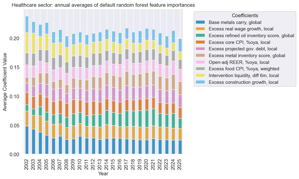
xcatx = hlc_dict["signal_name"]
secname = hlc_dict["sector_name"]

so_hlc.coefs_stackedbarplot(
    name=xcatx,
    ftrs=list(hlc_importances.columns[:10]),
    ftrs_renamed=cat_label_dict,
    title=f"{secname} sector: annual averages of default random forest feature importances",
)

Signal quality check

xcatx = [hlc_dict["signal_name"], hlc_dict["ret"]]
cidx = hlc_dict["cidx"]
secname = hlc_dict["sector_name"]

cr_hlc = msp.CategoryRelations(
    df=dfx,
    xcats=xcatx,
    cids=cidx,
    freq=hlc_dict["freq"],
    blacklist=hlc_dict["black"],
    lag=1,
    xcat_aggs=["last", "sum"],
    slip=1,
)

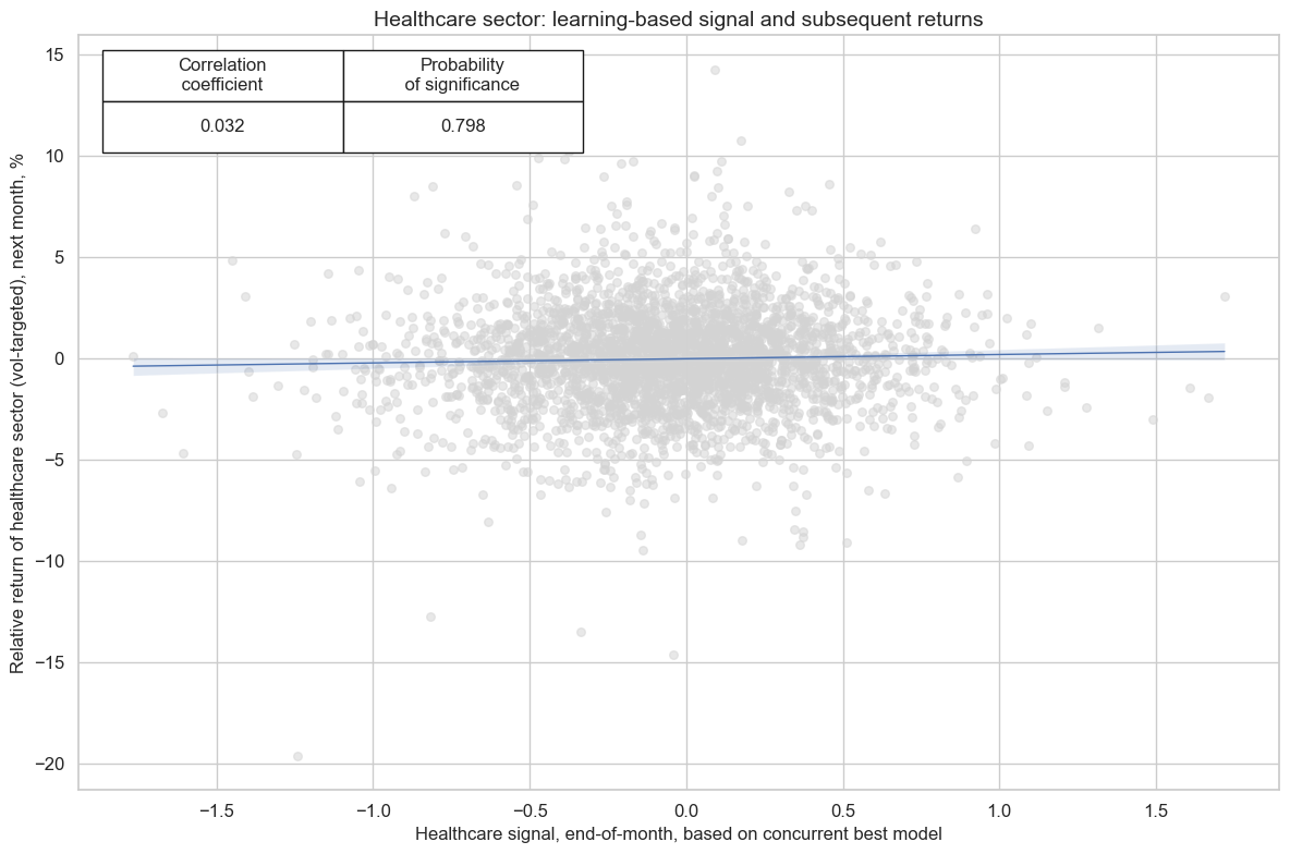
cr_hlc.reg_scatter(
    title=f"{secname} sector: learning-based signal and subsequent returns",
    labels=False,
    prob_est="map",
    xlab=f"{secname} signal, end-of-month, based on concurrent best model",
    ylab=f"Relative return of {secname.lower()} sector (vol-targeted), next month, %",
    coef_box="upper left",
    size=(12, 8),
)

xcatx = [hlc_dict["signal_name"]]
cidx = hlc_dict["cidx"]
secname = hlc_dict["sector_name"]
signal_name = hlc_dict["signal_name"]
pnl_name = hlc_dict["pnl_name"]

pnl_hlc = msn.NaivePnL(
    df=dfx,
    ret=hlc_dict["ret"],
    sigs=xcatx,
    cids=cidx,
    start=default_start_date,
    blacklist=hlc_dict["black"],
    bms=["USD_EQXR_NSA"],
)

for xcat in xcatx:
    pnl_hlc.make_pnl(
        sig=xcat,
        sig_op="zn_score_pan",
        rebal_freq="monthly",
        neutral="zero",
        rebal_slip=1,
        vol_scale=None,
        thresh=2,
        pnl_name=pnl_name,
    )
pnl_hlc.make_long_pnl(
    vol_scale=None, label=f"{secname} always long versus all-sector basket"
)

pnl_hlc.plot_pnls(
    pnl_cats=pnl_hlc.pnl_names,
    title=f"{secname} sector: naive PnLs of positions versus all-sector basket",
    title_fontsize=14,
)

hlc_dict["pnls"] = pnl_hlc
pnl_hlc.evaluate_pnls(pnl_cats=pnl_hlc.pnl_names)

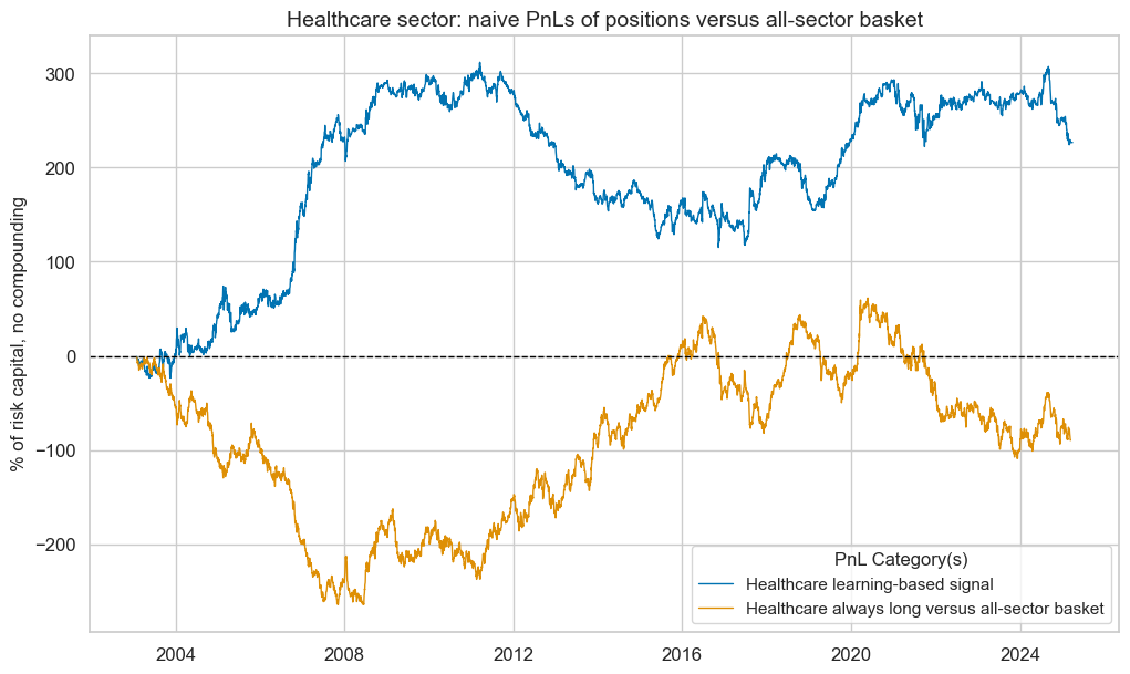
xcat	Healthcare learning-based signal	Healthcare always long versus all-sector basket
Return %	10.222537	-4.044239
St. Dev. %	36.745511	38.50816
Sharpe Ratio	0.278198	-0.105023
Sortino Ratio	0.398907	-0.150517
Max 21-Day Draw %	-40.391137	-47.409795
Max 6-Month Draw %	-82.460974	-93.207315
Peak to Trough Draw %	-196.363809	-262.724098
Top 5% Monthly PnL Share	1.461796	-4.156891
USD_EQXR_NSA correl	0.025846	-0.159044
Traded Months	267	267

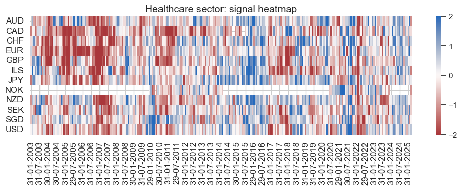
pnl_name = hlc_dict["pnl_name"]
secname = hlc_dict["sector_name"]

pnl_hlc.signal_heatmap(
    pnl_name=pnl_name,
    figsize=(12, 3),
    title=f"{secname} sector: signal heatmap",
)

Financials

Factor selection and signal generation

sector = "FIN"

fin_dict = {
    "sector_name": sector_labels[sector],
    "signal_name": f"{sector}SOL",
    "pnl_name": f"{sector_labels[sector]} learning-based signal",
    "xcatx": macroz,
    "cidx": cids_eq,
    "ret": f"EQC{sector}{default_target_type}",
    "freq": "M",
    "black": sector_blacklist[sector],
    "srr": None,
    "pnls": None,
}

xcatx = fin_dict["xcatx"] + [fin_dict["ret"]]
cidx = fin_dict["cidx"]

so_fin = msl.SignalOptimizer(
    df=dfx,
    xcats=xcatx,
    cids=cidx,
    blacklist=fin_dict["black"],
    freq=fin_dict["freq"],
    lag=1,
    xcat_aggs=["last", "sum"],
)

secname = fin_dict["sector_name"]
signal_name = fin_dict["signal_name"]

so_fin.calculate_predictions(
    name=signal_name,
    models=default_models,
    scorers=default_metric,
    hyperparameters=default_hparam_grid,
    inner_splitters=default_splitter,
    test_size=default_test_size,
    min_cids=default_min_cids,
    min_periods=default_min_periods,
    n_jobs_outer=-1,
    split_functions=default_split_functions,
)
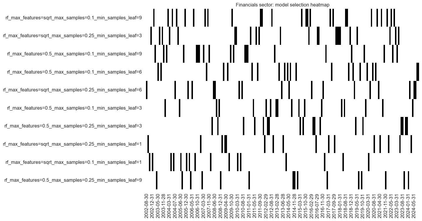
so_fin.models_heatmap(
    signal_name,
    cap=10,
    title=f"{secname} sector: model selection heatmap",
)

# Store signals
dfa = so_fin.get_optimized_signals()
dfx = msm.update_df(dfx, dfa)

fin_importances = (
    so_fin.feature_importances.describe()
    .iloc[:, 1:]
    .sort_values(by="mean", axis=1, ascending=False)
)

fin_importances

	BMLCOCRY_SAVT10_21DMA_ZN	XGGDGDPRATIOX10_NSA_ZN	REEROADJ_NSA_P1M12ML1_ZN	REFIXINVCSCORE_SA_ZN	CCSCORE_SA_ZN	XNRSALES_SA_P1M1ML12_3MMA_ZN	CXPI_NSA_P1M12ML1_ZN	XRRSALES_SA_P1M1ML12_3MMA_WG_ZN	XCPIC_SA_P1M1ML12_ZN	RYLDIRS05Y_NSA_ZN	...	XRPCONS_SA_P1M1ML12_3MMA_ZN	UNEMPLRATE_SA_3MMAv5YMA_WG_ZN	RIR_NSA_ZN	XRGDPTECH_SA_P1M1ML12_3MMA_ZN	UNEMPLRATE_NSA_3MMA_D1M1ML12_WG_ZN	XEMPL_NSA_P1M1ML12_3MMA_WG_ZN	XPCREDITBN_SJA_P1M1ML12_WG_ZN	XEMPL_NSA_P1M1ML12_3MMA_ZN	INTLIQGDP_NSA_D1M1ML1_ZN	XRGDPTECH_SA_P1M1ML12_3MMA_WG_ZN
count	271.000000	271.000000	271.000000	271.000000	271.000000	271.000000	271.000000	271.000000	271.000000	271.000000	...	271.000000	271.000000	271.000000	271.000000	271.000000	271.000000	271.000000	271.000000	271.000000	271.000000
mean	0.033372	0.025287	0.023579	0.023166	0.021470	0.021100	0.020746	0.020217	0.020046	0.019836	...	0.015416	0.015063	0.015060	0.015057	0.014955	0.014866	0.014655	0.014585	0.014475	0.013548
min	0.010865	0.004436	0.009034	0.003472	0.005645	0.006083	0.006847	0.005977	0.000000	0.005035	...	0.004102	0.002416	0.004604	0.003904	0.000000	0.000000	0.003381	0.003631	0.000000	0.001632
25%	0.027656	0.021381	0.019419	0.017802	0.018313	0.018005	0.018185	0.017301	0.017408	0.016759	...	0.013452	0.013413	0.012890	0.013293	0.012199	0.013143	0.013017	0.012837	0.012398	0.011708
50%	0.031273	0.023962	0.021537	0.023353	0.021124	0.020685	0.020399	0.019593	0.019095	0.019420	...	0.015217	0.015100	0.015275	0.014994	0.014086	0.014942	0.014668	0.014678	0.014073	0.013921
75%	0.037369	0.027731	0.025729	0.027977	0.024535	0.023980	0.023038	0.022346	0.021670	0.022126	...	0.017081	0.016805	0.017201	0.016782	0.017015	0.017023	0.016298	0.016837	0.016570	0.015091
max	0.077338	0.055350	0.060381	0.038759	0.036812	0.043096	0.037422	0.060037	0.037514	0.045437	...	0.036349	0.025588	0.026185	0.030416	0.039819	0.030730	0.025728	0.022955	0.030388	0.029012
std	0.009122	0.006131	0.007212	0.007033	0.005216	0.004871	0.004253	0.004962	0.004339	0.005024	...	0.003325	0.003413	0.003587	0.003272	0.004550	0.003251	0.003280	0.003126	0.003767	0.003065

8 rows × 56 columns

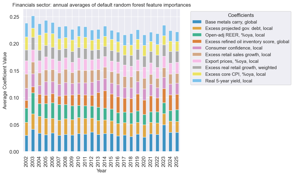
xcatx = fin_dict["signal_name"]
secname = fin_dict["sector_name"]

so_fin.coefs_stackedbarplot(
    name=xcatx,
    ftrs=list(fin_importances.columns[:10]),
    ftrs_renamed=cat_label_dict,
    title=f"{secname} sector: annual averages of default random forest feature importances",
)

Signal quality check

xcatx = [fin_dict["signal_name"], fin_dict["ret"]]
cidx = fin_dict["cidx"]
secname = fin_dict["sector_name"]

cr_fin = msp.CategoryRelations(
    df=dfx,
    xcats=xcatx,
    cids=cidx,
    freq=fin_dict["freq"],
    blacklist=fin_dict["black"],
    lag=1,
    xcat_aggs=["last", "sum"],
    slip=1,
)

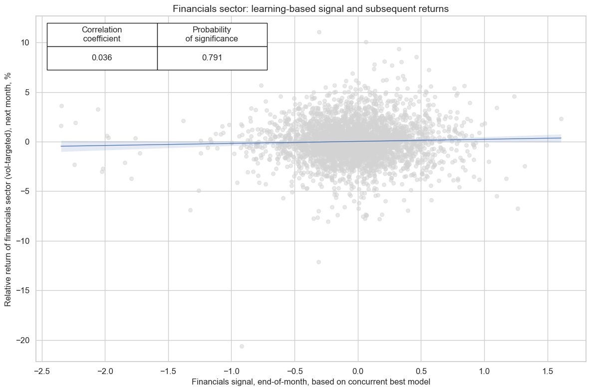
cr_fin.reg_scatter(
    title=f"{secname} sector: learning-based signal and subsequent returns",
    labels=False,
    prob_est="map",
    xlab=f"{secname} signal, end-of-month, based on concurrent best model",
    ylab=f"Relative return of {secname.lower()} sector (vol-targeted), next month, %",
    coef_box="upper left",
    size=(12, 8),
)

xcatx = [fin_dict["signal_name"]]
cidx = fin_dict["cidx"]
secname = fin_dict["sector_name"]
signal_name = fin_dict["signal_name"]
pnl_name = fin_dict["pnl_name"]

pnl_fin = msn.NaivePnL(
    df=dfx,
    ret=fin_dict["ret"],
    sigs=xcatx,
    cids=cidx,
    start=default_start_date,
    blacklist=fin_dict["black"],
    bms=["USD_EQXR_NSA"],
)

for xcat in xcatx:
    pnl_fin.make_pnl(
        sig=xcat,
        sig_op="zn_score_pan",
        rebal_freq="monthly",
        neutral="zero",
        rebal_slip=1,
        vol_scale=None,
        thresh=2,
        pnl_name=pnl_name,
    )
pnl_fin.make_long_pnl(
    vol_scale=None, label=f"{secname} always long versus all-sector basket"
)

pnl_fin.plot_pnls(
    pnl_cats=pnl_fin.pnl_names,
    title=f"{secname} sector: naive PnLs of positions versus all-sector basket",
    title_fontsize=14,
)

fin_dict["pnls"] = pnl_fin
pnl_fin.evaluate_pnls(pnl_cats=pnl_fin.pnl_names)

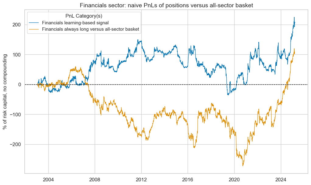
xcat	Financials learning-based signal	Financials always long versus all-sector basket
Return %	9.365027	4.921724
St. Dev. %	37.156358	38.288158
Sharpe Ratio	0.252044	0.128544
Sortino Ratio	0.354122	0.187923
Max 21-Day Draw %	-73.040887	-76.126375
Max 6-Month Draw %	-102.512582	-96.122679
Peak to Trough Draw %	-185.572225	-332.744644
Top 5% Monthly PnL Share	2.115025	3.978115
USD_EQXR_NSA correl	-0.062463	0.220494
Traded Months	267	267

xcatx = fin_dict["signal_name"]
pnl_name = fin_dict["pnl_name"]
secname = fin_dict["sector_name"]

pnl_fin.signal_heatmap(
    pnl_name=pnl_name,
    figsize=(12, 3),
    title=f"{secname} sector: signal heatmap",
)

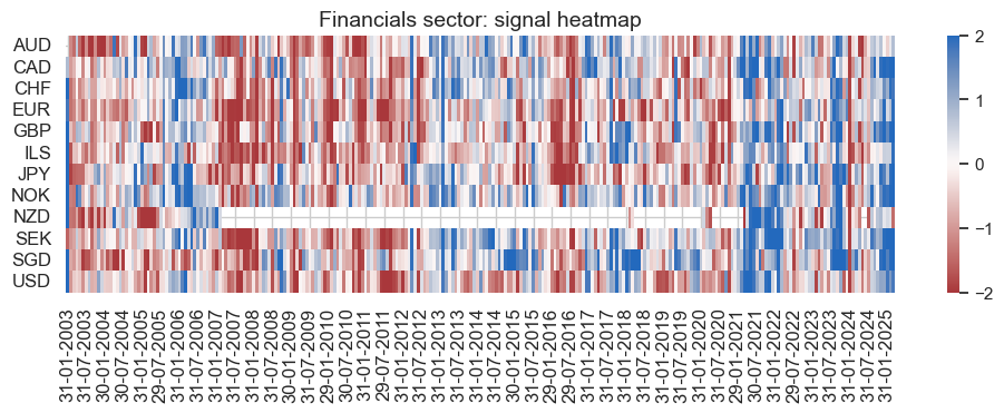
Technology

Factor selection and signal generation

sector = "ITE"

ite_dict = {
    "sector_name": sector_labels[sector],
    "signal_name": f"{sector}SOL",
    "pnl_name": f"{sector_labels[sector]} learning-based signal",
    "xcatx": macroz,
    "cidx": cids_eq,
    "ret": f"EQC{sector}{default_target_type}",
    "freq": "M",
    "black": sector_blacklist[sector],
    "srr": None,
    "pnls": None,
}

xcatx = ite_dict["xcatx"] + [ite_dict["ret"]]
cidx = ite_dict["cidx"]

so_ite = msl.SignalOptimizer(
    df=dfx,
    xcats=xcatx,
    cids=cidx,
    blacklist=ite_dict["black"],
    freq=ite_dict["freq"],
    lag=1,
    xcat_aggs=["last", "sum"],
)

secname = ite_dict["sector_name"]
signal_name = ite_dict["signal_name"]

so_ite.calculate_predictions(
    name=signal_name,
    models=default_models,
    scorers=default_metric,
    hyperparameters=default_hparam_grid,
    inner_splitters=default_splitter,
    test_size=default_test_size,
    min_cids=default_min_cids,
    min_periods=default_min_periods,
    n_jobs_outer=-1,
    split_functions=default_split_functions,
)
so_ite.models_heatmap(
    signal_name,
    cap=10,
    title=f"{secname} sector: model selection heatmap",
)

# Store signals
dfa = so_ite.get_optimized_signals()
dfx = msm.update_df(dfx, dfa)

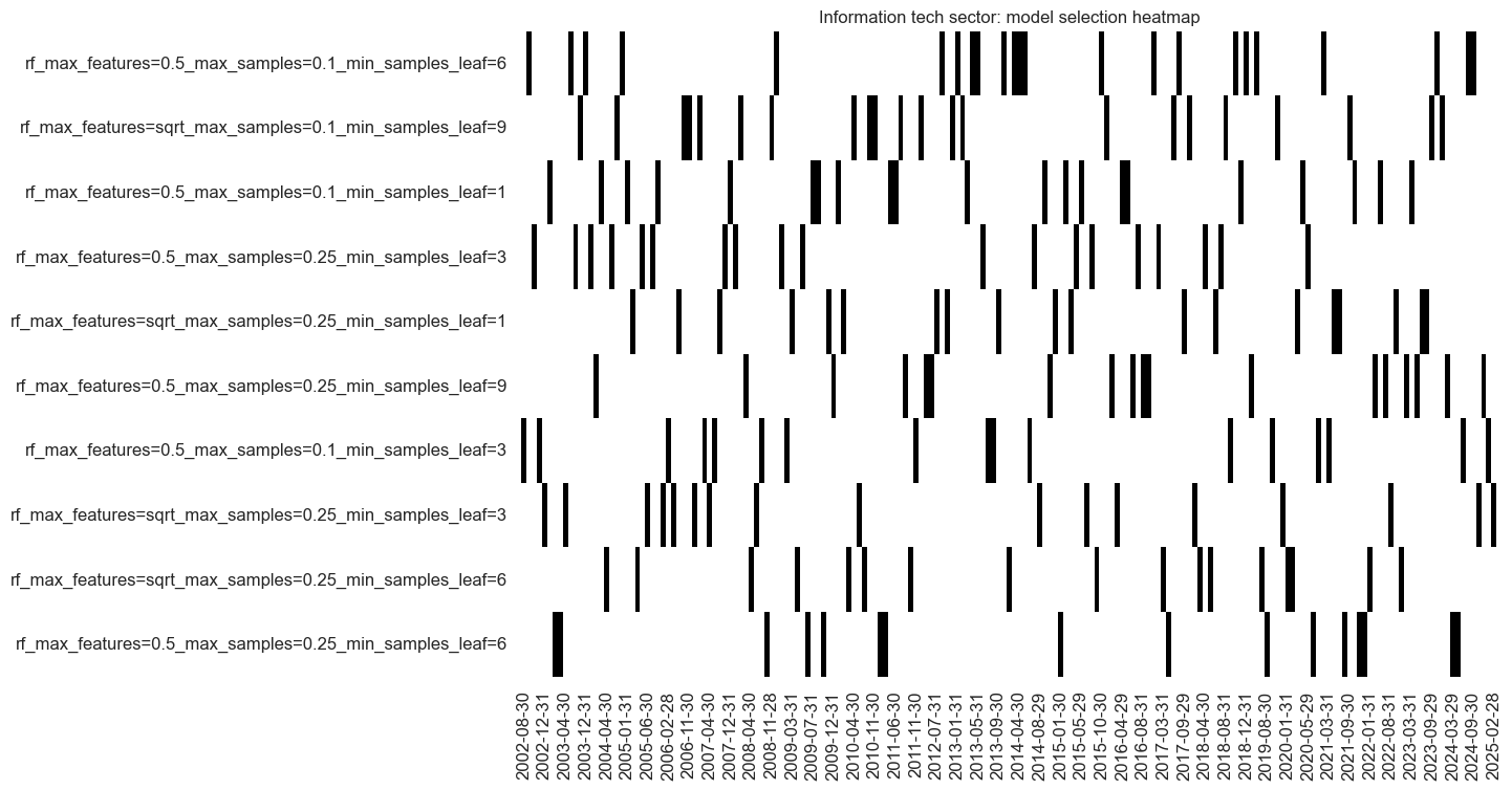
ite_importances = (
    so_ite.feature_importances.describe()
    .iloc[:, 1:]
    .sort_values(by="mean", axis=1, ascending=False)
)

ite_importances

	CCSCORE_SA_WG_ZN	CCSCORE_SA_ZN	BASEXINVCSCORE_SA_ZN	RYLDIRS05Y_NSA_ZN	XCPIC_SA_P1M1ML12_ZN	BMLCOCRY_SAVT10_21DMA_ZN	XRWAGES_NSA_P1M1ML12_ZN	CCSCORE_SA_D3M3ML3_ZN	XCSTR_SA_P1M1ML12_3MMA_ZN	RYLDIRS02Y_NSA_ZN	...	XRPCONS_SA_P1M1ML12_3MMA_ZN	UNEMPLRATE_NSA_3MMA_D1M1ML12_ZN	XPCREDITBN_SJA_P1M1ML12_WG_ZN	CMPI_NSA_P1M12ML1_ZN	XEMPL_NSA_P1M1ML12_3MMA_ZN	XRGDPTECH_SA_P1M1ML12_3MMA_WG_ZN	MBCSCORE_SA_WG_ZN	XCPIE_SA_P1M1ML12_ZN	INTLIQGDP_NSA_D1M1ML1_ZN	INTLIQGDP_NSA_D1M1ML6_ZN
count	271.000000	271.000000	271.000000	271.000000	271.000000	271.000000	271.000000	271.000000	271.000000	271.000000	...	271.000000	271.000000	271.000000	271.000000	271.000000	271.000000	271.000000	271.000000	271.000000	271.000000
mean	0.030261	0.024013	0.023329	0.022619	0.021590	0.021239	0.020491	0.020355	0.020341	0.020250	...	0.015429	0.015360	0.015276	0.015233	0.014980	0.014925	0.014924	0.014871	0.014065	0.013750
min	0.001367	0.008941	0.003188	0.008631	0.000000	0.007969	0.001486	0.011236	0.003893	0.006764	...	0.002832	0.002292	0.000000	0.003810	0.003766	0.000000	0.000000	0.004875	0.002708	0.000000
25%	0.023197	0.019194	0.020209	0.017678	0.019226	0.018037	0.017841	0.017503	0.018101	0.016691	...	0.013621	0.013347	0.013101	0.013465	0.012837	0.012859	0.013265	0.013249	0.011501	0.012052
50%	0.027825	0.022868	0.023367	0.021071	0.021651	0.020599	0.020715	0.019846	0.020271	0.020051	...	0.015666	0.015124	0.015139	0.015402	0.015002	0.014911	0.015292	0.015171	0.013466	0.013527
75%	0.034228	0.027893	0.026217	0.024486	0.023901	0.023165	0.023632	0.022112	0.022773	0.023418	...	0.017126	0.016941	0.017525	0.017263	0.016794	0.016986	0.017015	0.016764	0.016105	0.015282
max	0.084165	0.056244	0.041380	0.077280	0.034307	0.069902	0.033888	0.048929	0.044928	0.055986	...	0.026680	0.044387	0.029174	0.040348	0.031202	0.034112	0.023317	0.025330	0.027336	0.030871
std	0.010217	0.006499	0.005452	0.008363	0.004174	0.006465	0.004914	0.004525	0.004095	0.006028	...	0.003263	0.004046	0.003689	0.003768	0.003654	0.003837	0.003340	0.003006	0.003831	0.003146

8 rows × 56 columns

xcatx = ite_dict["signal_name"]
secname = ite_dict["sector_name"]

so_ite.coefs_stackedbarplot(
    name=xcatx,
    ftrs=list(ite_importances.columns[:10]),
    ftrs_renamed=cat_label_dict,
    title=f"{secname} sector: annual averages of default random forest feature importances",
)

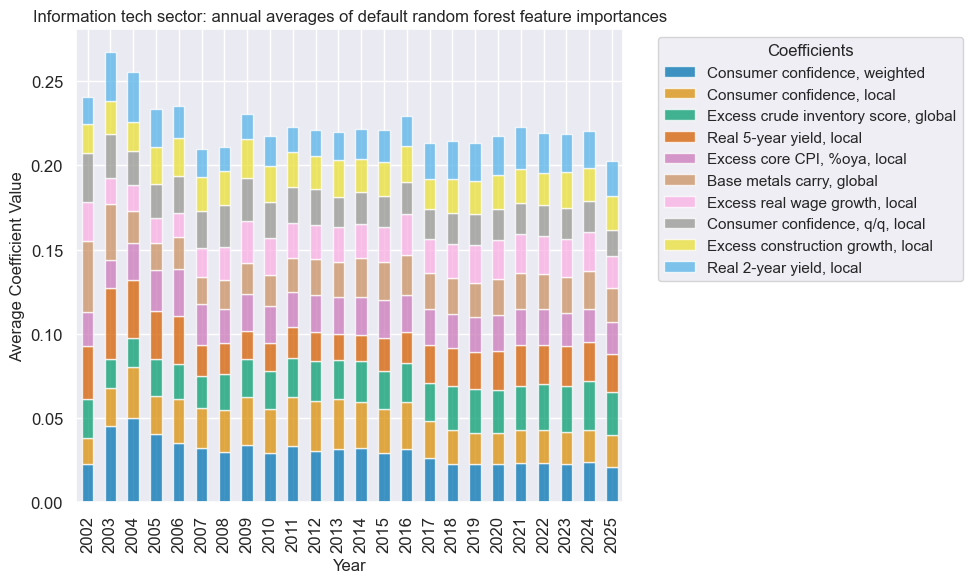
Signal quality check

xcatx = [ite_dict["signal_name"], ite_dict["ret"]]
cidx = ite_dict["cidx"]
secname = ite_dict["sector_name"]

cr_ite = msp.CategoryRelations(
    df=dfx,
    xcats=xcatx,
    cids=cidx,
    freq=ite_dict["freq"],
    blacklist=ite_dict["black"],
    lag=1,
    xcat_aggs=["last", "sum"],
    slip=1,
)

cr_ite.reg_scatter(
    title=f"{secname} sector: learning-based signal and subsequent returns",
    labels=False,
    prob_est="map",
    xlab=f"{secname} signal, end-of-month, based on concurrent best model",
    ylab=f"Relative return of {secname.lower()} sector (vol-targeted), next month, %",
    coef_box="upper left",
    size=(12, 8),
)

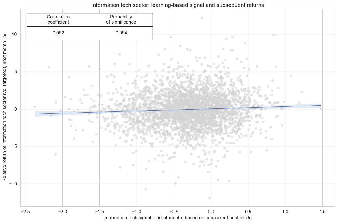
xcatx = [ite_dict["signal_name"]]
cidx = ite_dict["cidx"]
secname = ite_dict["sector_name"]
signal_name = ite_dict["signal_name"]
pnl_name = ite_dict["pnl_name"]

pnl_ite = msn.NaivePnL(
    df=dfx,
    ret=ite_dict["ret"],
    sigs=xcatx,
    cids=cidx,
    start=default_start_date,
    blacklist=ite_dict["black"],
    bms=["USD_EQXR_NSA"],
)

for xcat in xcatx:
    pnl_ite.make_pnl(
        sig=xcat,
        sig_op="zn_score_pan",
        rebal_freq="monthly",
        neutral="zero",
        rebal_slip=1,
        vol_scale=None,
        thresh=2,
        pnl_name=pnl_name,
    )
pnl_ite.make_long_pnl(
    vol_scale=None, label=f"{secname} always long versus all-sector basket"
)

pnl_ite.plot_pnls(
    pnl_cats=pnl_ite.pnl_names,
    title=f"{secname} sector: naive PnLs of positions versus all-sector basket",
    title_fontsize=14,
)

ite_dict["pnls"] = pnl_ite
pnl_ite.evaluate_pnls(pnl_cats=pnl_ite.pnl_names)

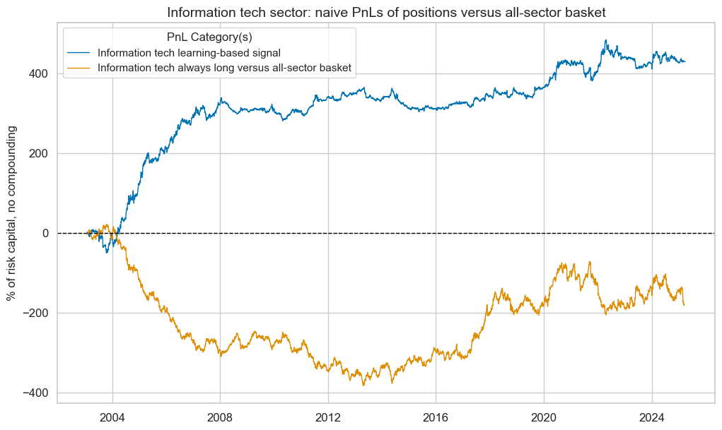
xcat	Information tech learning-based signal	Information tech always long versus all-sector basket
Return %	19.387719	-8.140115
St. Dev. %	29.531038	37.685315
Sharpe Ratio	0.65652	-0.216002
Sortino Ratio	0.947428	-0.298073
Max 21-Day Draw %	-33.439709	-44.700924
Max 6-Month Draw %	-55.095888	-116.166222
Peak to Trough Draw %	-73.379864	-404.663283
Top 5% Monthly PnL Share	0.801098	-2.012503
USD_EQXR_NSA correl	-0.010929	0.034275
Traded Months	267	267

pnl_name = ite_dict["pnl_name"]
secname = ite_dict["sector_name"]

pnl_ite.signal_heatmap(
    pnl_name=pnl_name,
    figsize=(12, 3),
    title=f"{secname} sector: signal heatmap",
)

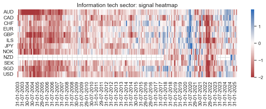
Communication

Factor selection and signal generation

sector = "CSR"

csr_dict = {
    "sector_name": sector_labels[sector],
    "signal_name": f"{sector}SOL",
    "pnl_name": f"{sector_labels[sector]} learning-based signal",
    "xcatx": macroz,
    "cidx": cids_eq,
    "ret": f"EQC{sector}{default_target_type}",
    "freq": "M",
    "black": sector_blacklist[sector],
    "srr": None,
    "pnls": None,
}

xcatx = csr_dict["xcatx"] + [csr_dict["ret"]]
cidx = csr_dict["cidx"]

so_csr = msl.SignalOptimizer(
    df=dfx,
    xcats=xcatx,
    cids=cidx,
    blacklist=csr_dict["black"],
    freq=csr_dict["freq"],
    lag=1,
    xcat_aggs=["last", "sum"],
)

secname = csr_dict["sector_name"]
signal_name = csr_dict["signal_name"]

so_csr.calculate_predictions(
    name=signal_name,
    models=default_models,
    scorers=default_metric,
    hyperparameters=default_hparam_grid,
    inner_splitters=default_splitter,
    test_size=default_test_size,
    min_cids=default_min_cids,
    min_periods=default_min_periods,
    n_jobs_outer=-1,
    split_functions=default_split_functions,
)
so_csr.models_heatmap(
    signal_name,
    cap=10,
    title=f"{secname} sector: model selection heatmap",
)

# Store signals
dfa = so_csr.get_optimized_signals()
dfx = msm.update_df(dfx, dfa)

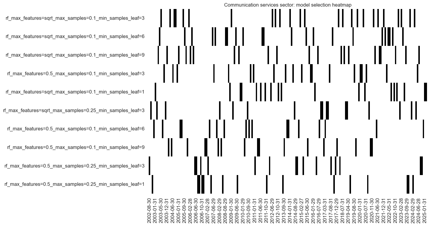
csr_importances = (
    so_csr.feature_importances.describe()
    .iloc[:, 1:]
    .sort_values(by="mean", axis=1, ascending=False)
)

csr_importances

	BMLCOCRY_SAVT10_21DMA_ZN	BASEXINVCSCORE_SA_ZN	BMLXINVCSCORE_SA_ZN	REEROADJ_NSA_P1M12ML1_ZN	XCPIF_SA_P1M1ML12_WG_ZN	XCPIC_SA_P1M1ML12_ZN	REFIXINVCSCORE_SA_ZN	SBCSCORE_SA_D3M3ML3_ZN	CCSCORE_SA_WG_ZN	XGGDGDPRATIOX10_NSA_ZN	...	RYLDIRS02Y_NSA_ZN	XPCREDITBN_SJA_P1M1ML12_ZN	RIR_NSA_ZN	XRPCONS_SA_P1M1ML12_3MMA_ZN	XRRSALES_SA_P1M1ML12_3MMA_WG_ZN	UNEMPLRATE_NSA_3MMA_D1M1ML12_WG_ZN	MBCSCORE_SA_ZN	INTLIQGDP_NSA_D1M1ML6_ZN	MBCSCORE_SA_WG_ZN	INTLIQGDP_NSA_D1M1ML1_ZN
count	271.000000	271.000000	271.000000	271.000000	271.000000	271.000000	271.000000	271.000000	271.000000	271.000000	...	271.000000	271.000000	271.000000	271.000000	271.000000	271.000000	271.000000	271.000000	271.000000	271.000000
mean	0.036693	0.024477	0.021401	0.021264	0.021232	0.019959	0.019796	0.019587	0.019304	0.018930	...	0.016126	0.016100	0.015976	0.015905	0.015837	0.015744	0.015281	0.015043	0.014910	0.012920
min	0.017953	0.007102	0.005521	0.009010	0.007010	0.008086	0.003762	0.005060	0.006814	0.008000	...	0.005501	0.004550	0.000000	0.007630	0.005802	0.004954	0.004175	0.006478	0.005579	0.000000
25%	0.027478	0.020074	0.018817	0.018998	0.018816	0.018079	0.017863	0.017368	0.017367	0.016708	...	0.013961	0.013990	0.013771	0.014191	0.013955	0.013567	0.013501	0.013150	0.013153	0.010968
50%	0.032192	0.024018	0.021243	0.021064	0.020305	0.019843	0.019769	0.019381	0.019102	0.019062	...	0.015962	0.015885	0.016558	0.015977	0.015562	0.015107	0.015618	0.014986	0.014996	0.012811
75%	0.039888	0.029479	0.024336	0.023413	0.022853	0.022015	0.021920	0.021557	0.021270	0.021513	...	0.018421	0.017812	0.018606	0.017574	0.017475	0.017389	0.017436	0.016834	0.016693	0.015015
max	0.106062	0.045552	0.032073	0.035086	0.052603	0.029376	0.037136	0.036590	0.049853	0.031693	...	0.040416	0.031015	0.023952	0.025420	0.037431	0.032887	0.029713	0.026712	0.028042	0.022384
std	0.014006	0.007156	0.004529	0.003621	0.005087	0.003306	0.004092	0.003989	0.003802	0.003992	...	0.003831	0.003526	0.003775	0.002850	0.003414	0.003742	0.003319	0.003340	0.002903	0.003233

8 rows × 56 columns

xcatx = csr_dict["signal_name"]
secname = csr_dict["sector_name"]

so_csr.coefs_stackedbarplot(
    name=xcatx,
    ftrs=list(csr_importances.columns[:10]),
    ftrs_renamed=cat_label_dict,
    title=f"{secname} sector: annual averages of default random forest feature importances",
)

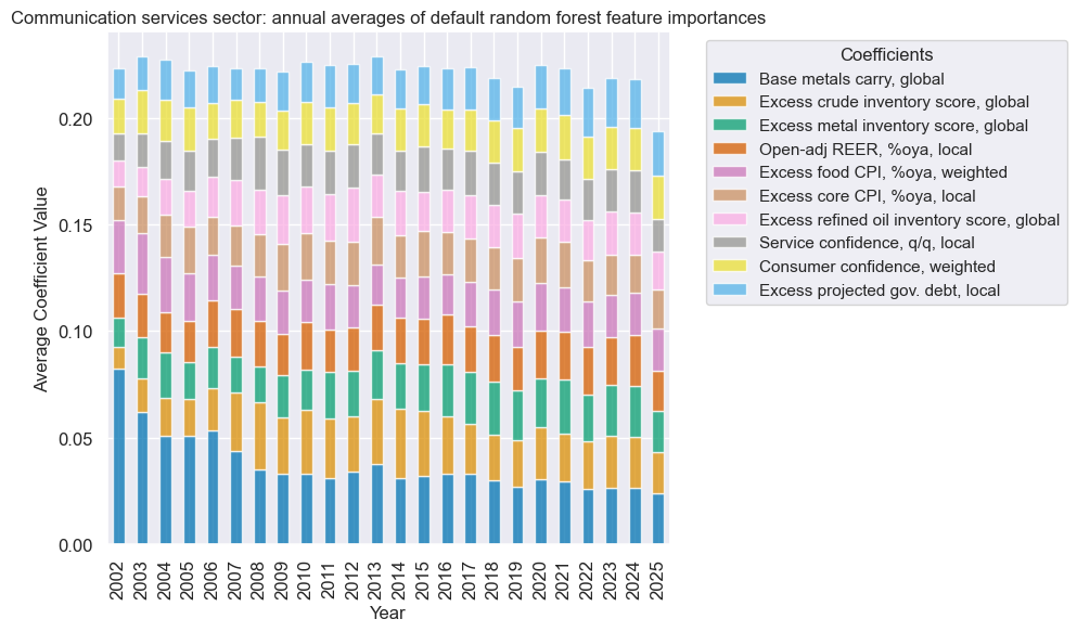
Signal quality check

xcatx = [csr_dict["signal_name"], csr_dict["ret"]]
cidx = csr_dict["cidx"]
secname = csr_dict["sector_name"]

cr_csr = msp.CategoryRelations(
    df=dfx,
    xcats=xcatx,
    cids=cidx,
    freq=csr_dict["freq"],
    blacklist=csr_dict["black"],
    lag=1,
    xcat_aggs=["last", "sum"],
    slip=1,
)

cr_csr.reg_scatter(
    title=f"{secname} sector: learning-based signal and subsequent returns",
    labels=False,
    prob_est="map",
    xlab=f"{secname} signal, end-of-month, based on concurrent best model",
    ylab=f"Relative return of {secname.lower()} sector (vol-targeted), next month, %",
    coef_box="upper left",
    size=(12, 8),
)

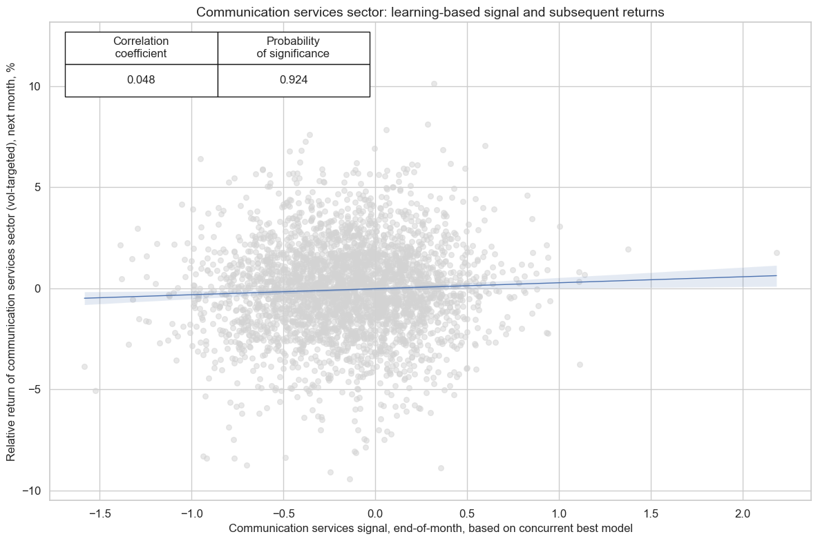
xcatx = [csr_dict["signal_name"]]
cidx = csr_dict["cidx"]
secname = csr_dict["sector_name"]
signal_name = csr_dict["signal_name"]
pnl_name = csr_dict["pnl_name"]

pnl_csr = msn.NaivePnL(
    df=dfx,
    ret=csr_dict["ret"],
    sigs=xcatx,
    cids=cidx,
    start=default_start_date,
    blacklist=csr_dict["black"],
    bms=["USD_EQXR_NSA"],
)

for xcat in xcatx:
    pnl_csr.make_pnl(
        sig=xcat,
        sig_op="zn_score_pan",
        rebal_freq="monthly",
        neutral="zero",
        rebal_slip=1,
        vol_scale=None,
        thresh=2,
        pnl_name=pnl_name,
    )
pnl_csr.make_long_pnl(
    vol_scale=None, label=f"{secname} always long versus all-sector basket"
)

pnl_csr.plot_pnls(
    pnl_cats=pnl_csr.pnl_names,
    title=f"{secname} sector: naive PnLs of positions versus all-sector basket",
    title_fontsize=14,
)

csr_dict["pnls"] = pnl_csr
pnl_csr.evaluate_pnls(pnl_cats=pnl_csr.pnl_names)

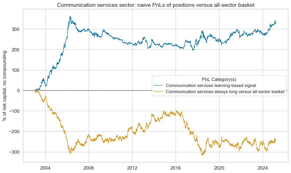
xcat	Communication services learning-based signal	Communication services always long versus all-sector basket
Return %	14.888869	-11.148616
St. Dev. %	31.790794	35.84342
Sharpe Ratio	0.468339	-0.311037
Sortino Ratio	0.675637	-0.440682
Max 21-Day Draw %	-35.326814	-41.34344
Max 6-Month Draw %	-52.062922	-110.518234
Peak to Trough Draw %	-168.65979	-322.629621
Top 5% Monthly PnL Share	1.177937	-1.32878
USD_EQXR_NSA correl	-0.002595	-0.043378
Traded Months	267	267

pnl_name = csr_dict["pnl_name"]
secname = csr_dict["sector_name"]

pnl_csr.signal_heatmap(
    pnl_name=pnl_name,
    figsize=(12, 3),
    title=f"{secname} sector: signal heatmap",
)

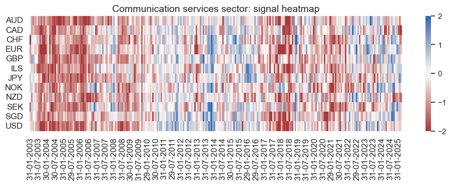
Utilities

Factor selection and signal generation

sector = "UTL"

utl_dict = {
    "sector_name": sector_labels[sector],
    "signal_name": f"{sector}SOL",
    "pnl_name": f"{sector_labels[sector]} learning-based signal",
    "xcatx": macroz,
    "cidx": cids_eq,
    "ret": f"EQC{sector}{default_target_type}",
    "freq": "M",
    "black": sector_blacklist[sector],
    "srr": None,
    "pnls": None,
}

xcatx = utl_dict["xcatx"] + [utl_dict["ret"]]
cidx = utl_dict["cidx"]

so_utl = msl.SignalOptimizer(
    df=dfx,
    xcats=xcatx,
    cids=cidx,
    blacklist=utl_dict["black"],
    freq=utl_dict["freq"],
    lag=1,
    xcat_aggs=["last", "sum"],
)

secname = utl_dict["sector_name"]
signal_name = utl_dict["signal_name"]

so_utl.calculate_predictions(
    name=signal_name,
    models=default_models,
    scorers=default_metric,
    hyperparameters=default_hparam_grid,
    inner_splitters=default_splitter,
    test_size=default_test_size,
    min_cids=default_min_cids,
    min_periods=default_min_periods,
    n_jobs_outer=-1,
    split_functions=default_split_functions,
)
so_utl.models_heatmap(
    signal_name,
    cap=10,
    title=f"{secname} sector: model selection heatmap",
)

# Store signals
dfa = so_utl.get_optimized_signals()
dfx = msm.update_df(dfx, dfa)

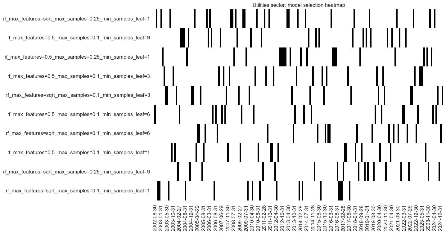
utl_importances = (
    so_utl.feature_importances.describe()
    .iloc[:, 1:]
    .sort_values(by="mean", axis=1, ascending=False)
)

utl_importances

	XCPIC_SA_P1M1ML12_ZN	XGGDGDPRATIOX10_NSA_ZN	REEROADJ_NSA_P1M12ML1_ZN	BMLXINVCSCORE_SA_ZN	BASEXINVCSCORE_SA_ZN	CCSCORE_SA_WG_ZN	CCSCORE_SA_D3M3ML3_ZN	BMLCOCRY_SAVT10_21DMA_ZN	SBCSCORE_SA_ZN	XCSTR_SA_P1M1ML12_3MMA_ZN	...	XPPIH_NSA_P1M1ML12_ZN	XNRSALES_SA_P1M1ML12_3MMA_WG_ZN	RIR_NSA_ZN	UNEMPLRATE_NSA_3MMA_D1M1ML12_WG_ZN	XCPIE_SA_P1M1ML12_ZN	XEMPL_NSA_P1M1ML12_3MMA_WG_ZN	XRGDPTECH_SA_P1M1ML12_3MMA_WG_ZN	INTLIQGDP_NSA_D1M1ML6_ZN	UNEMPLRATE_SA_3MMAv5YMA_WG_ZN	INTLIQGDP_NSA_D1M1ML1_ZN
count	271.000000	271.000000	271.000000	271.000000	271.000000	271.000000	271.000000	271.000000	271.000000	271.000000	...	271.000000	271.000000	271.000000	271.000000	271.000000	271.000000	271.000000	271.000000	271.000000	271.000000
mean	0.024699	0.022147	0.021922	0.021921	0.021238	0.021040	0.020656	0.020600	0.020064	0.019866	...	0.016128	0.015954	0.015927	0.015291	0.015114	0.014828	0.014549	0.014293	0.014061	0.012332
min	0.000000	0.009021	0.004621	0.000000	0.002127	0.010302	0.007687	0.008099	0.003351	0.000000	...	0.005405	0.003963	0.000000	0.000000	0.003377	0.005392	0.002376	0.006362	0.005790	0.003598
25%	0.021077	0.018753	0.019286	0.016556	0.018523	0.017831	0.017319	0.018326	0.017675	0.017419	...	0.013696	0.013317	0.013528	0.012997	0.013192	0.012961	0.012494	0.012393	0.011988	0.010356
50%	0.024948	0.021813	0.021636	0.022302	0.021292	0.020335	0.019818	0.020575	0.019748	0.019223	...	0.015647	0.015594	0.016061	0.015143	0.015275	0.014745	0.014365	0.014220	0.013743	0.012149
75%	0.028483	0.024660	0.024206	0.027384	0.024114	0.023360	0.022784	0.022789	0.022146	0.022070	...	0.017834	0.017979	0.018652	0.017200	0.017344	0.016729	0.016443	0.016293	0.015777	0.014055
max	0.039321	0.045679	0.045228	0.040423	0.034466	0.045139	0.047516	0.041862	0.051541	0.037113	...	0.034939	0.035284	0.042584	0.033917	0.026552	0.026037	0.032041	0.025885	0.028715	0.030566
std	0.006037	0.005227	0.004880	0.007543	0.005092	0.005045	0.005222	0.004027	0.004425	0.004469	...	0.003867	0.004197	0.004503	0.003987	0.003473	0.003058	0.003494	0.003065	0.003371	0.003502

8 rows × 56 columns

xcatx = utl_dict["signal_name"]
secname = utl_dict["sector_name"]

so_utl.coefs_stackedbarplot(
    name=xcatx,
    ftrs=list(utl_importances.columns[:10]),
    ftrs_renamed=cat_label_dict,
    title=f"{secname} sector: annual averages of default random forest feature importances",
)

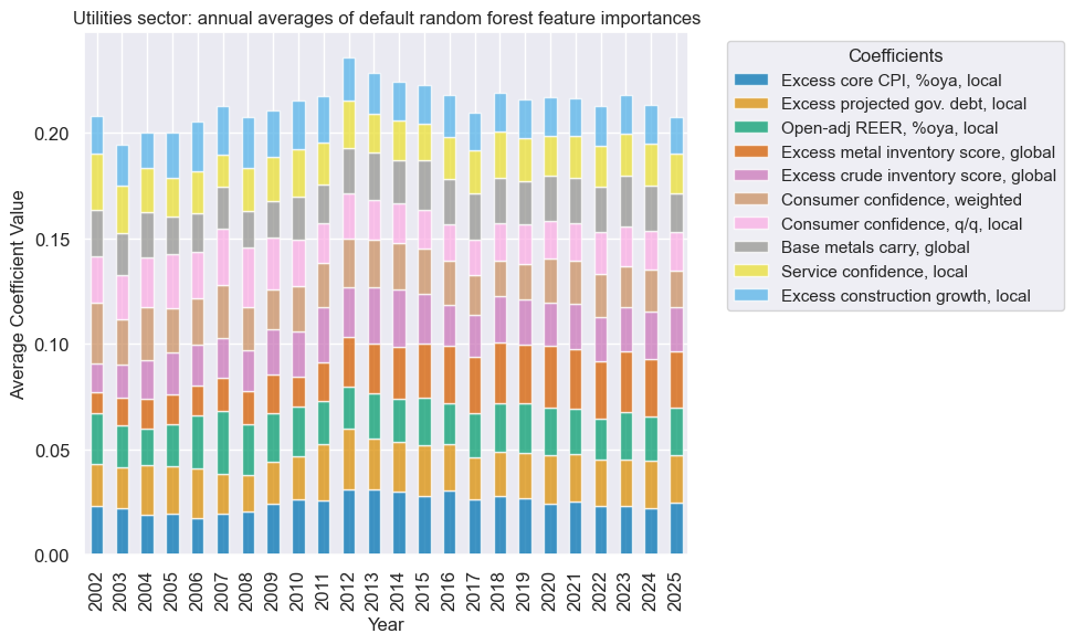
Signal quality check

xcatx = [utl_dict["signal_name"], utl_dict["ret"]]
cidx = utl_dict["cidx"]
secname = utl_dict["sector_name"]

cr_utl = msp.CategoryRelations(
    df=dfx,
    xcats=xcatx,
    cids=cidx,
    freq=utl_dict["freq"],
    blacklist=utl_dict["black"],
    lag=1,
    xcat_aggs=["last", "sum"],
    slip=1,
)

cr_utl.reg_scatter(
    title=f"{secname} sector: learning-based signal and subsequent returns",
    labels=False,
    prob_est="map",
    xlab=f"{secname} signal, end-of-month, based on concurrent best model",
    ylab=f"Relative return of {secname.lower()} sector (vol-targeted), next month, %",
    coef_box="upper left",
    size=(12, 8),
)

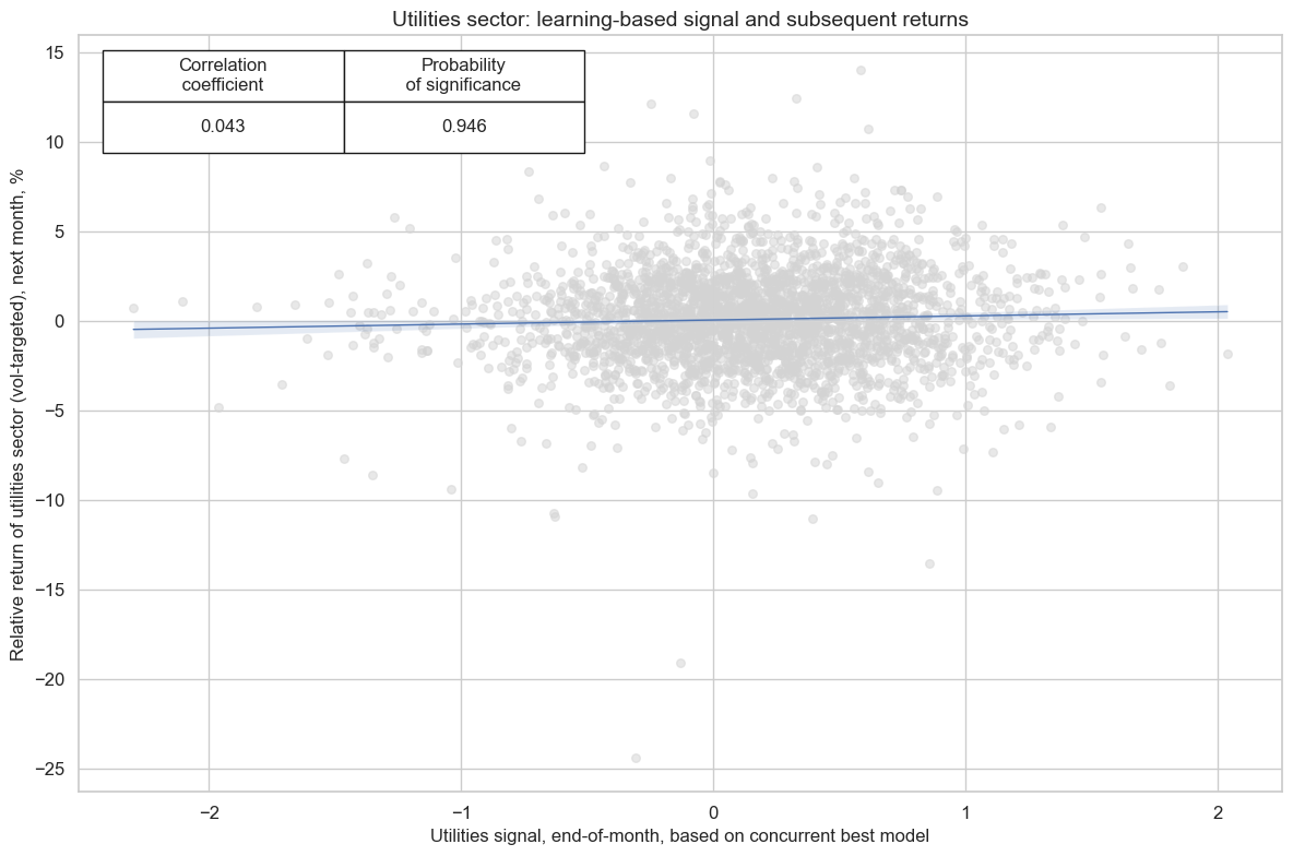
xcatx = [utl_dict["signal_name"]]
cidx = utl_dict["cidx"]
secname = utl_dict["sector_name"]
signal_name = utl_dict["signal_name"]
pnl_name = utl_dict["pnl_name"]

pnl_utl = msn.NaivePnL(
    df=dfx,
    ret=utl_dict["ret"],
    sigs=xcatx,
    cids=cidx,
    start=default_start_date,
    blacklist=utl_dict["black"],
    bms=["USD_EQXR_NSA"],
)

for xcat in xcatx:
    pnl_utl.make_pnl(
        sig=xcat,
        sig_op="zn_score_pan",
        rebal_freq="monthly",
        neutral="zero",
        rebal_slip=1,
        vol_scale=None,
        thresh=2,
        pnl_name=pnl_name,
    )
pnl_utl.make_long_pnl(
    vol_scale=None, label=f"{secname} always long versus all-sector basket"
)

pnl_utl.plot_pnls(
    pnl_cats=pnl_utl.pnl_names,
    title=f"{secname} sector: naive PnLs of positions versus all-sector basket",
    title_fontsize=14,
)

utl_dict["pnls"] = pnl_utl
pnl_utl.evaluate_pnls(pnl_cats=pnl_utl.pnl_names)

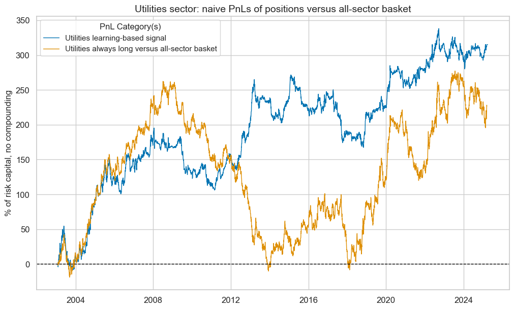
xcat	Utilities learning-based signal	Utilities always long versus all-sector basket
Return %	14.221555	10.241575
St. Dev. %	32.206642	39.653484
Sharpe Ratio	0.441572	0.258277
Sortino Ratio	0.634653	0.377312
Max 21-Day Draw %	-34.741035	-45.235513
Max 6-Month Draw %	-76.122475	-93.980448
Peak to Trough Draw %	-104.192426	-272.563373
Top 5% Monthly PnL Share	1.124063	1.843926
USD_EQXR_NSA correl	-0.094479	-0.196373
Traded Months	267	267

pnl_name = utl_dict["pnl_name"]
secname = utl_dict["sector_name"]

pnl_utl.signal_heatmap(
    pnl_name=pnl_name,
    figsize=(12, 3),
    title=f"{secname} sector: signal heatmap",
)

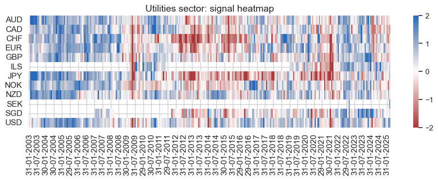
Real estate

Factor selection and signal generation

sector = "REL"

rel_dict = {
    "sector_name": sector_labels[sector],
    "signal_name": f"{sector}SOL",
    "pnl_name": f"{sector_labels[sector]} learning-based signal",
    "xcatx": macroz,
    "cidx": cids_eq,
    "ret": f"EQC{sector}{default_target_type}",
    "freq": "M",
    "black": sector_blacklist[sector],
    "srr": None,
    "pnls": None,
}

xcatx = rel_dict["xcatx"] + [rel_dict["ret"]]
cidx = rel_dict["cidx"]

so_rel = msl.SignalOptimizer(
    df=dfx,
    xcats=xcatx,
    cids=cidx,
    blacklist=rel_dict["black"],
    freq=rel_dict["freq"],
    lag=1,
    xcat_aggs=["last", "sum"],
)

secname = rel_dict["sector_name"]
signal_name = rel_dict["signal_name"]

so_rel.calculate_predictions(
    name=signal_name,
    models=default_models,
    scorers=default_metric,
    hyperparameters=default_hparam_grid,
    inner_splitters=default_splitter,
    test_size=default_test_size,
    min_cids=default_min_cids,
    min_periods=default_min_periods,
    n_jobs_outer=-1,
    split_functions=default_split_functions,
)
so_rel.models_heatmap(
    signal_name,
    cap=10,
    title=f"{secname} sector: model selection heatmap",
)

# Store signals
dfa = so_rel.get_optimized_signals()
dfx = msm.update_df(dfx, dfa)

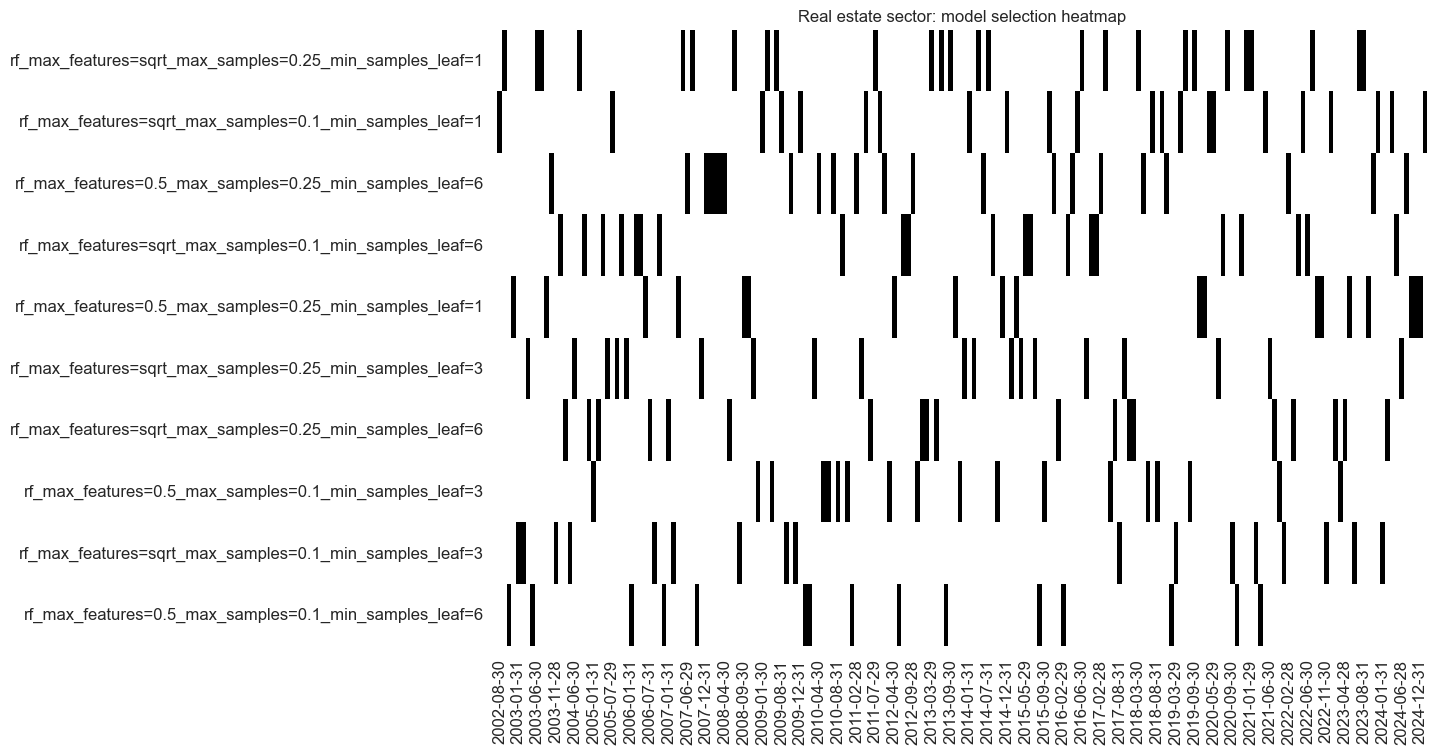
rel_importances = (
    so_rel.feature_importances.describe()
    .iloc[:, 1:]
    .sort_values(by="mean", axis=1, ascending=False)
)

rel_importances

	BMLCOCRY_SAVT10_21DMA_ZN	RSLOPEMIDDLE_NSA_ZN	BASEXINVCSCORE_SA_ZN	SBCSCORE_SA_D3M3ML3_ZN	REEROADJ_NSA_P1M12ML1_ZN	CCSCORE_SA_D3M3ML3_WG_ZN	CCSCORE_SA_D3M3ML3_ZN	XCPIE_SA_P1M1ML12_WG_ZN	BMLXINVCSCORE_SA_ZN	XGGDGDPRATIOX10_NSA_ZN	...	MBCSCORE_SA_ZN	XNRSALES_SA_P1M1ML12_3MMA_WG_ZN	CTOT_NSA_P1M12ML1_ZN	XNRSALES_SA_P1M1ML12_3MMA_ZN	XPPIH_NSA_P1M1ML12_ZN	XRPCONS_SA_P1M1ML12_3MMA_ZN	XRGDPTECH_SA_P1M1ML12_3MMA_WG_ZN	XIP_SA_P1M1ML12_3MMA_WG_ZN	XIP_SA_P1M1ML12_3MMA_ZN	INTLIQGDP_NSA_D1M1ML1_ZN
count	271.000000	271.000000	271.000000	271.000000	271.000000	271.000000	271.000000	271.000000	271.000000	271.000000	...	271.000000	271.000000	271.000000	271.000000	271.000000	271.000000	271.000000	271.000000	271.000000	271.000000
mean	0.031318	0.024617	0.021564	0.021460	0.020621	0.020412	0.020273	0.019713	0.019438	0.019259	...	0.015914	0.015854	0.015844	0.015843	0.015795	0.015708	0.015647	0.014766	0.014519	0.011117
min	0.007034	0.012426	0.005993	0.007465	0.007313	0.011612	0.009965	0.008585	0.002531	0.002839	...	0.002635	0.004350	0.007116	0.005200	0.002624	0.008284	0.005482	0.001973	0.006622	0.001459
25%	0.026673	0.019865	0.018143	0.018675	0.018359	0.017410	0.017667	0.017177	0.016867	0.016309	...	0.013856	0.014016	0.014196	0.014047	0.014329	0.013423	0.013885	0.012999	0.012757	0.009671
50%	0.030136	0.022131	0.021660	0.020941	0.020229	0.019427	0.019686	0.019713	0.020495	0.018169	...	0.016362	0.016012	0.015593	0.015797	0.015672	0.015429	0.015311	0.014730	0.014529	0.011383
75%	0.035547	0.026537	0.024795	0.023576	0.022556	0.022009	0.022120	0.022094	0.022770	0.020903	...	0.018224	0.017562	0.017066	0.017594	0.017679	0.017456	0.017477	0.016525	0.016044	0.012800
max	0.056073	0.092364	0.040660	0.039646	0.041894	0.048476	0.040364	0.030912	0.031073	0.040282	...	0.024917	0.026088	0.035300	0.025686	0.028305	0.028764	0.028938	0.029810	0.030046	0.017757
std	0.008259	0.008476	0.005603	0.004297	0.004220	0.005154	0.004282	0.003956	0.005136	0.004923	...	0.003455	0.002902	0.003159	0.002932	0.003251	0.003321	0.003156	0.003190	0.003042	0.002609

8 rows × 56 columns

xcatx = rel_dict["signal_name"]
secname = rel_dict["sector_name"]

so_rel.coefs_stackedbarplot(
    name=xcatx,
    ftrs=list(rel_importances.columns[:10]),
    ftrs_renamed=cat_label_dict,
    title=f"{secname} sector: annual averages of default random forest feature importances",
)

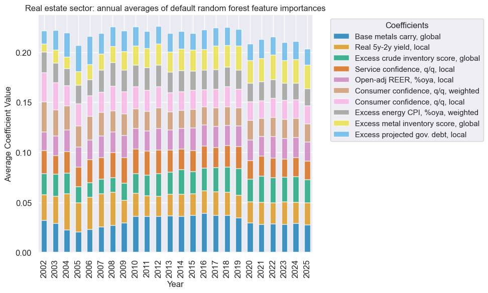
Signal quality check

xcatx = [rel_dict["signal_name"], rel_dict["ret"]]
cidx = rel_dict["cidx"]
secname = rel_dict["sector_name"]

cr_rel = msp.CategoryRelations(
    df=dfx,
    xcats=xcatx,
    cids=cidx,
    freq=rel_dict["freq"],
    blacklist=rel_dict["black"],
    lag=1,
    xcat_aggs=["last", "sum"],
    slip=1,
)

cr_rel.reg_scatter(
    title=f"{secname} sector: learning-based signal and subsequent returns",
    labels=False,
    prob_est="map",
    xlab=f"{secname} signal, end-of-month, based on concurrent best model",
    ylab=f"Relative return of {secname.lower()} sector (vol-targeted), next month, %",
    coef_box="upper left",
    size=(12, 8),
)

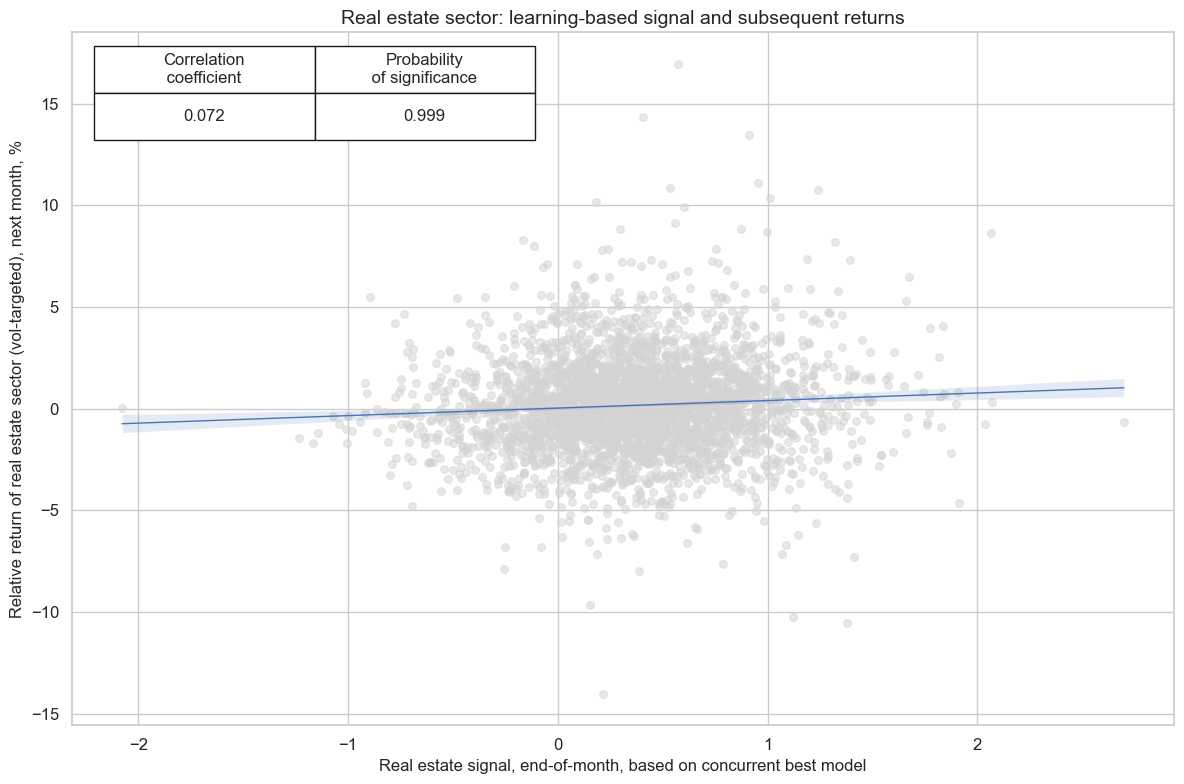
xcatx = [rel_dict["signal_name"]]
cidx = rel_dict["cidx"]
secname = rel_dict["sector_name"]
signal_name = rel_dict["signal_name"]
pnl_name = rel_dict["pnl_name"]

pnl_rel = msn.NaivePnL(
    df=dfx,
    ret=rel_dict["ret"],
    sigs=xcatx,
    cids=cidx,
    start=default_start_date,
    blacklist=rel_dict["black"],
    bms=["USD_EQXR_NSA"],
)

for xcat in xcatx:
    pnl_rel.make_pnl(
        sig=xcat,
        sig_op="zn_score_pan",
        rebal_freq="monthly",
        neutral="zero",
        rebal_slip=1,
        vol_scale=None,
        thresh=3,
        pnl_name=pnl_name,
    )
pnl_rel.make_long_pnl(
    vol_scale=None, label=f"{secname} always long versus all-sector basket"
)

pnl_rel.plot_pnls(
    pnl_cats=pnl_rel.pnl_names,
    title=f"{secname} sector: naive PnLs of positions versus all-sector basket",
    title_fontsize=14,
)

rel_dict["pnls"] = pnl_rel
pnl_rel.evaluate_pnls(pnl_cats=pnl_rel.pnl_names)

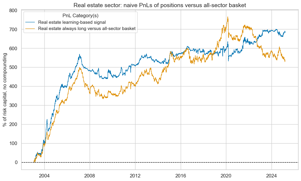
xcat	Real estate learning-based signal	Real estate always long versus all-sector basket
Return %	30.862946	24.25139
St. Dev. %	37.173338	42.658717
Sharpe Ratio	0.830244	0.568498
Sortino Ratio	1.212027	0.811584
Max 21-Day Draw %	-93.712629	-107.121602
Max 6-Month Draw %	-67.848759	-123.928869
Peak to Trough Draw %	-130.190976	-237.128421
Top 5% Monthly PnL Share	0.739336	0.949022
USD_EQXR_NSA correl	-0.045183	-0.054054
Traded Months	267	267

pnl_name = rel_dict["pnl_name"]
secname = rel_dict["sector_name"]

pnl_rel.signal_heatmap(
    pnl_name=pnl_name,
    figsize=(12, 3),
    title=f"{secname} sector: signal heatmap",
)

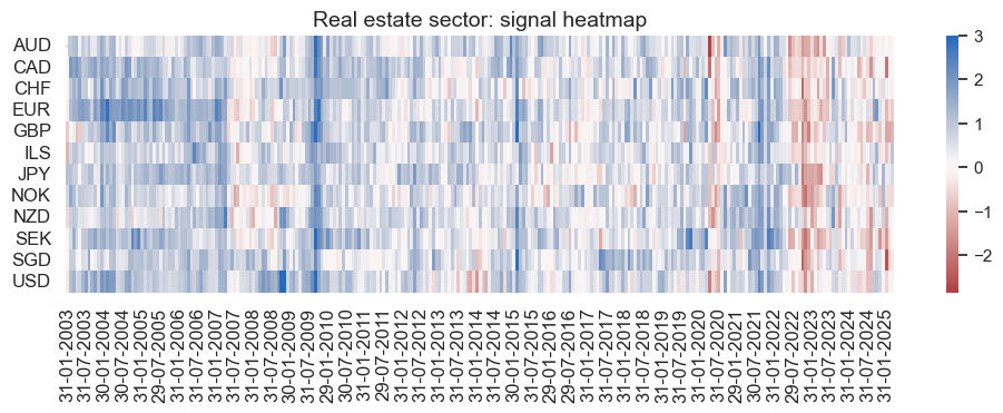
Summary

Sector-specific signals and returns

sec_catregs = {
    "enr": cr_enr,
    "mat": cr_mat,
    "ind": cr_ind,
    "cod": cr_cod, 
    "cos": cr_cos,
    "hlc": cr_hlc,
    "fin": cr_fin,
    "ite": cr_ite, 
    "csr": cr_csr,
    "utl": cr_utl, 
    "rel": cr_rel,
}


msv.multiple_reg_scatter(
    cat_rels=list(sec_catregs.values()),
    ncol=3,
    nrow=4,
    figsize=(15, 15),
    title="Random forest macro signals and subsequent sectoral equity returns, 11 currency areas, since 2003",
    title_xadj=0.5,
    title_yadj=0.99,
    title_fontsize=20,
    xlab="Sector-specific random forest regression signal based on macro-quantamental categories",
    ylab="Sector return versus equal weighted local index (all vol-targeted), next month %",
    coef_box="lower right",
    prob_est="map",
    single_chart=True,
    subplot_titles=[sector_labels[sector.upper()] for sector in sec_catregs.keys()],
)

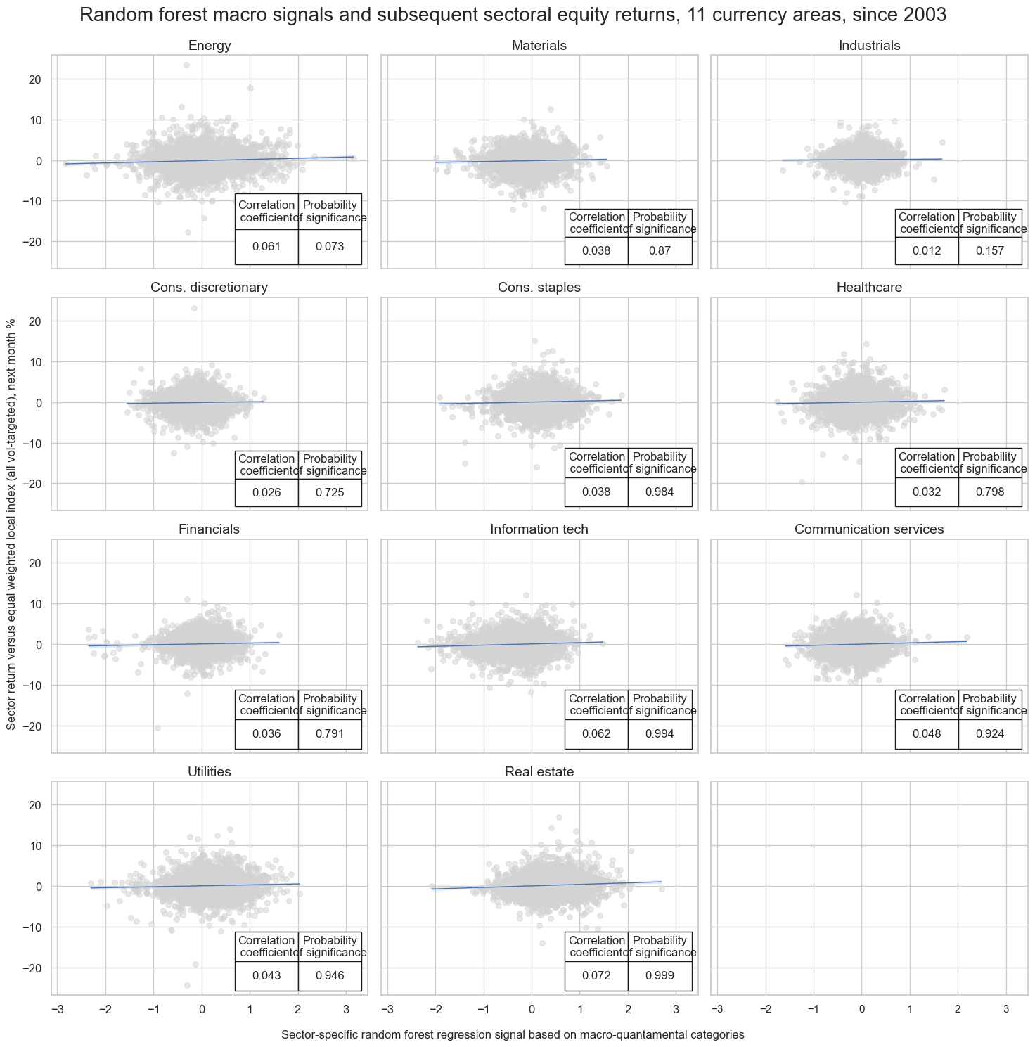
Combined cross-sector trading PnL

sec_pnls = {
    "enr": pnl_enr,
    "mat": pnl_mat,
    "ind": pnl_ind,
    "cod": pnl_cod,
    "cos": pnl_cos,
    "hlc": pnl_hlc,
    "fin": pnl_fin,
    "ite": pnl_ite,
    "csr": pnl_csr,
    "utl": pnl_utl,
    "rel": pnl_rel,
}

ma_pnl = msn.MultiPnL()
for sec, pnl in sec_pnls.items():
    ma_pnl.add_pnl(
        pnl, pnl_xcats=[f"{sector_labels[sec.upper()]} learning-based signal"]
    )

ma_pnl.plot_pnls(
    pnl_xcats=[
        f"{sector_labels[sec.upper()]} learning-based signal" for sec in sec_pnls.keys()
    ],
    title="Naive PnLs for random-forest-based relative sector strategies",
    xcat_labels=[sector_labels[sec.upper()] for sec in sec_pnls.keys()],
)

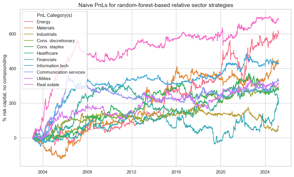
cpname = "Simple average PnL of relative sector strategies based on machine learning and macro signals"

macro_sector_pnl = ma_pnl.combine_pnls(
    pnl_xcats=[
        f"{sector_labels[sec.upper()]} learning-based signal" for sec in sec_pnls.keys()
    ],
    composite_pnl_xcat=cpname,
    weights=None,
)
ma_pnl.plot_pnls(
    [cpname],
    title="Cumulative naive PnL value of random forest-based cross-sectoral equity allocation",
)

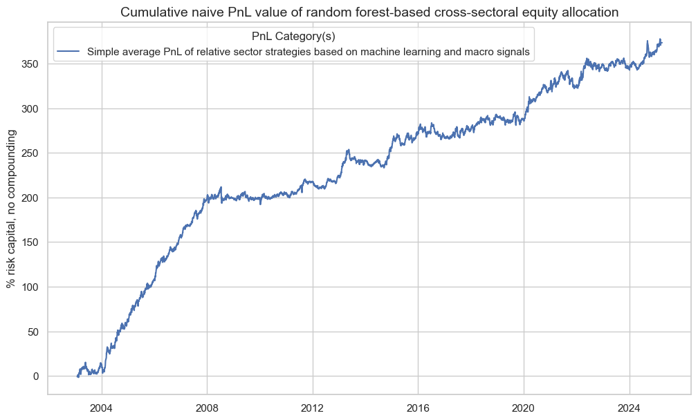
tbr = ma_pnl.evaluate_pnls()
tbr = tbr.rename(
    columns={
        **{
            f"{sector_labels[sec.upper()]} learning-based signal/EQC{sec.upper()}R_VT10vALL": f"{sector_labels[sec.upper()]}"
            for sec in sec_pnls.keys()
        },
        **{
            "Simple average PnL of relative sector strategies based on machine learning and macro signals": "Simple average"
        },
    }
)

# selected_rows = ["Return %", "St. Dev. %", "Sharpe Ratio", "Sortino Ratio", "USD_EQXR_NSA correl"]
selected_columns = ["Simple average"] + [
    sector_labels[sec.upper()] for sec in sec_pnls.keys()
]
selected_pnl_stats = tbr.loc[:, selected_columns].T

selected_pnl_stats.columns

cols = [
    "Sharpe Ratio",
    "Sortino Ratio",
    "Top 5% Monthly PnL Share",
    "USD_EQXR_NSA correl",
]
display(selected_pnl_stats[cols].style.format("{:.2f}"))

	Sharpe Ratio	Sortino Ratio	Top 5% Monthly PnL Share	USD_EQXR_NSA correl
Simple average	1.18	1.70	0.40	nan
Energy	0.47	0.68	0.95	-0.06
Materials	0.44	0.62	1.18	-0.02
Industrials	0.11	0.16	3.59	-0.00
Cons. discretionary	0.42	0.61	1.05	-0.01
Cons. staples	0.34	0.48	1.44	-0.06
Healthcare	0.28	0.40	1.46	0.03
Financials	0.25	0.35	2.12	-0.06
Information tech	0.66	0.95	0.80	-0.01
Communication services	0.47	0.68	1.18	-0.00
Utilities	0.44	0.63	1.12	-0.09
Real estate	0.83	1.21	0.74	-0.05

Appendix

Appendix 1 - Macro quantamental indicators description

# Convert the dictionary to an HTML table with custom inline CSS
html_table = cat_labels.to_html(index=True, table_id="custom_table")

# Inject CSS to align text to the left and reduce font size
css = """
<style>
#custom_table th, #custom_table td {
    text-align: left;
    font-size: 12px; /* Adjust the font size as needed */
}
</style>
"""

# Display the styled HTML table
HTML(css + html_table)

		Label	Description	Geography
Group	Category
Business surveys	CBCSCORE_SA_D3M3ML3_WG_ZN	Construction confidence, q/q	Construction business confidence score, seas. adjusted, change q/q	weighted
	CBCSCORE_SA_D3M3ML3_ZN	Construction confidence, q/q	Construction business confidence score, seas. adjusted, change q/q	local
	CBCSCORE_SA_WG_ZN	Construction confidence	Construction business confidence score, seas. adjusted	weighted
	CBCSCORE_SA_ZN	Construction confidence	Construction business confidence score, seas. adjusted	local
	MBCSCORE_SA_D3M3ML3_WG_ZN	Manufacturing confidence, q/q	Manufacturing business confidence score, seas. adj., change q/q	weighted
	MBCSCORE_SA_D3M3ML3_ZN	Manufacturing confidence, q/q	Manufacturing business confidence score, seas. adj., change q/q	local
	MBCSCORE_SA_WG_ZN	Manufacturing confidence	Manufacturing business confidence score, seasonally adjusted	weighted
	MBCSCORE_SA_ZN	Manufacturing confidence	Manufacturing business confidence score, seasonally adjusted	local
	SBCSCORE_SA_D3M3ML3_WG_ZN	Service confidence, q/q	Services business confidence score, seas. adjusted, change q/q	weighted
	SBCSCORE_SA_D3M3ML3_ZN	Service confidence, q/q	Services business confidence score, seas. adjusted, change q/q	local
	SBCSCORE_SA_WG_ZN	Service confidence	Services business confidence score, seasonally adjusted	weighted
	SBCSCORE_SA_ZN	Service confidence	Services business confidence score, seasonally adjusted	local
Commodity inventories	BASEXINVCSCORE_SA_ZN	Excess crude inventory score	Crude oil excess inventory z-score, seasonally adjusted	global
	BMLXINVCSCORE_SA_ZN	Excess metal inventory score	Base metal excess inventory z-score, seasonally adjusted	global
	REFIXINVCSCORE_SA_ZN	Excess refined oil inventory score	Refined oil product excess inventory z-score, seas. adjusted	global
Debt	CORPINTNETGDP_SA_D1Q1QL4_WG_ZN	Corporate debt servicing, %oya	Corporate net debt servicing-to-GDP ratio, seasonally-adjusted, %oya	weighted
	CORPINTNETGDP_SA_D1Q1QL4_ZN	Corporate debt servicing, %oya	Corporate net debt servicing-to-GDP ratio, seasonally-adjusted, %oya	local
	HHINTNETGDP_SA_D1M1ML12_WG_ZN	Households debt servicing, %oya	Households net debt servicing-to-GDP ratio, seasonally-adjusted, %oya	weighted
	HHINTNETGDP_SA_D1M1ML12_ZN	Households debt servicing, %oya	Households net debt servicing-to-GDP ratio, seasonally-adjusted, %oya	local
	XGGDGDPRATIOX10_NSA_ZN	Excess projected gov. debt	Government debt-to-GDP ratio proj. in 10 years, in excess of 100%	local
Exports	XEXPORTS_SA_P1M1ML12_3MMA_ZN	Excess export growth	Exports growth, %oya, 3mma, in excess of 5-year median GDP growth	local
Inflation - broad	XCPIC_SA_P1M1ML12_ZN	Excess core CPI, %oya	Core CPI, %oya, in excess of effective inflation target	local
	XCPIH_SA_P1M1ML12_ZN	Excess headline CPI, %oya	Headline CPI, %oya, in excess of effective inflation target	local
	XPPIH_NSA_P1M1ML12_ZN	Excess PPI, %oya	Producer price inflation, %oya, in excess of eff. inflation target	local
Inflation - specific	XCPIE_SA_P1M1ML12_WG_ZN	Excess energy CPI, %oya	Energy CPI, %oya, in excess of effective inflation target	weighted
	XCPIE_SA_P1M1ML12_ZN	Excess energy CPI, %oya	Energy CPI, %oya, in excess of effective inflation target	local
	XCPIF_SA_P1M1ML12_WG_ZN	Excess food CPI, %oya	Food CPI, %oya, in excess of effective inflation target	weighted
	XCPIF_SA_P1M1ML12_ZN	Excess food CPI, %oya	Food CPI, %oya, in excess of effective inflation target	local
Labour market	UNEMPLRATE_NSA_3MMA_D1M1ML12_WG_ZN	Unemployment rate, diff oya	Unemployment rate, change oya	weighted
	UNEMPLRATE_NSA_3MMA_D1M1ML12_ZN	Unemployment rate, diff oya	Unemployment rate, change oya	local
	UNEMPLRATE_SA_3MMAv5YMA_WG_ZN	Unemployment rate, diff vs 5yma	Unemployment rate, difference vs 5-year moving average	weighted
	UNEMPLRATE_SA_3MMAv5YMA_ZN	Unemployment rate, diff vs 5yma	Unemployment rate, difference vs 5-year moving average	local
	XEMPL_NSA_P1M1ML12_3MMA_WG_ZN	Excess employment growth	Employment growth, %oya, 3mma, in excess of population growth	weighted
	XEMPL_NSA_P1M1ML12_3MMA_ZN	Excess employment growth	Employment growth, %oya, 3mma, in excess of population growth	local
	XRWAGES_NSA_P1M1ML12_ZN	Excess real wage growth	Real wage growth, %oya, in excess of medium-term productivity growth	local
Market metrics	BMLCOCRY_SAVT10_21DMA_ZN	Base metals carry	Nominal carry for base metals basket, seasonally and vol-adjusted, 21 days moving average	global
	COXR_VT10vWTI_21DMA_ZN	Refined vs crude oil returns	Refined oil products vs crude oil vol-targeted return differential, 21 days moving average	global
	RIR_NSA_ZN	Real 1-month rate	Real 1-month interest rate	local
	RSLOPEMIDDLE_NSA_ZN	Real 5y-2y yield	Real IRS yield differentials, 5-years versus 2-years	local
	RYLDIRS02Y_NSA_ZN	Real 2-year yield	Real 2-year IRS yield	local
	RYLDIRS05Y_NSA_ZN	Real 5-year yield	Real 5-year IRS yield	local
Output growth	XCSTR_SA_P1M1ML12_3MMA_WG_ZN	Excess construction growth	Construction output, %oya, 3mma, in excess of 5-y median GDP growth	weighted
	XCSTR_SA_P1M1ML12_3MMA_ZN	Excess construction growth	Construction output, %oya, 3mma, in excess of 5-y median GDP growth	local
	XIP_SA_P1M1ML12_3MMA_WG_ZN	Excess industry growth	Industrial output, %oya, 3mma, in excess of 5-y median GDP growth	weighted
	XIP_SA_P1M1ML12_3MMA_ZN	Excess industry growth	Industrial output, %oya, 3mma, in excess of 5-y median GDP growth	local
	XRGDPTECH_SA_P1M1ML12_3MMA_WG_ZN	Excess GDP growth	Real GDP, %oya, 3mma, using HF data, in excess of 5-y med. GDP growth	weighted
	XRGDPTECH_SA_P1M1ML12_3MMA_ZN	Excess GDP growth	Real GDP, %oya, 3mma, using HF data, in excess of 5-y med. GDP growth	local
Private consumption	CCSCORE_SA_D3M3ML3_WG_ZN	Consumer confidence, q/q	Consumer confidence score, seasonally adjusted, change q/q	weighted
	CCSCORE_SA_D3M3ML3_ZN	Consumer confidence, q/q	Consumer confidence score, seasonally adjusted, change q/q	local
	CCSCORE_SA_WG_ZN	Consumer confidence	Consumer confidence score, seasonally adjusted	weighted
	CCSCORE_SA_ZN	Consumer confidence	Consumer confidence score, seasonally adjusted	local
	XNRSALES_SA_P1M1ML12_3MMA_WG_ZN	Excess retail sales growth	Nominal retail sales, %oya, 3mma, in excess of 5-y median GDP growth	weighted
	XNRSALES_SA_P1M1ML12_3MMA_ZN	Excess retail sales growth	Nominal retail sales, %oya, 3mma, in excess of 5-y median GDP growth	local
	XRPCONS_SA_P1M1ML12_3MMA_WG_ZN	Excess consumption growth	Real private consumption, %oya, 3mma, in excess of 5-y median GDP growth	weighted
	XRPCONS_SA_P1M1ML12_3MMA_ZN	Excess real consum growth	Real private consumption, %oya, 3mma, in excess of 5-y median GDP growth	local
	XRRSALES_SA_P1M1ML12_3MMA_WG_ZN	Excess real retail growth	Real retail sales, %oya, 3mma, in excess of 5-y median GDP growth	weighted
	XRRSALES_SA_P1M1ML12_3MMA_ZN	Excess real retail growth	Real retail sales, %oya, 3mma, in excess of 5-y median GDP growth	local
Private credit	INTLIQGDP_NSA_D1M1ML1_ZN	Intervention liquidity, diff m/m	Intervention liquidity to GDP ratio, change over the last month	local
	INTLIQGDP_NSA_D1M1ML6_ZN	Intervention liquidity, diff 6m	Intervention liquidity to GDP ratio, change overlast 6 months	local
	XPCREDITBN_SJA_P1M1ML12_WG_ZN	Excess credit growth	Private credit, %oya, 3mma, in excess of 5-y median GDP growth	weighted
	XPCREDITBN_SJA_P1M1ML12_ZN	Excess credit growth	Private credit, %oya, 3mma, in excess of 5-y median GDP growth	local
Real appreciation	CMPI_NSA_P1M12ML1_ZN	Import prices, %oya	Commodity-based import price index, %oya	local
	CTOT_NSA_P1M12ML1_ZN	Terms-of-trade, %oya	Commodity-based terms-of-trade, %oya	local
	CXPI_NSA_P1M12ML1_ZN	Export prices, %oya	Commodity-based export price index, %oya	local
	REEROADJ_NSA_P1M12ML1_ZN	Open-adj REER, %oya	Openness-adjusted real effective exchange rate, %oya	local