Economic surprise indicators: Primer and strategy example #
Get packages and JPMaQS data #
This notebook primarily relies on the standard packages available in the Python data science stack. However, there is an additional package
macrosynergy
that is required for two purposes:
-
Downloading JPMaQS data: The
macrosynergypackage facilitates the retrieval of JPMaQS data, which is used in the notebook. -
For the analysis of quantamental data and value propositions: The
macrosynergypackage provides functionality for performing quick analyses of quantamental data and exploring value propositions.
For detailed information and a comprehensive understanding of the
macrosynergy
package and its functionalities, please refer to the
“Introduction to Macrosynergy package”
notebook on the Macrosynergy Quantamental Academy or visit the following link on
Kaggle
.
import os
import numpy as np
import pandas as pd
import matplotlib.pyplot as plt
import seaborn as sns
import math

import json
import yaml
from timeit import default_timer as timer
from datetime import timedelta, date, datetime


import macrosynergy.management as msm
import macrosynergy.panel as msp
import macrosynergy.signal as mss
import macrosynergy.pnl as msn
import macrosynergy.visuals as msv

from macrosynergy.download import JPMaQSDownload


import warnings

warnings.simplefilter("ignore")
The JPMaQS indicators we consider are downloaded using the J.P. Morgan Dataquery API interface within the
macrosynergy
package. This is done by specifying ticker strings, formed by appending an indicator category code
<category>
to a currency area code
<cross_section>
. These constitute the main part of a full quantamental indicator ticker, taking the form
DB(JPMAQS,<cross_section>_<category>,<info>)
, where
<info>
denotes the time series of information for the given cross-section and category. The following types of information are available:
value
giving the latest available values for the indicator
eop_lag
referring to days elapsed since the end of the observation period
mop_lag
referring to the number of days elapsed since the mean observation period
grade
denoting a grade of the observation, giving a metric of real-time information quality.
After instantiating the
JPMaQSDownload
class within the
macrosynergy.download
module, one can use the
download(tickers,start_date,metrics)
method to easily download the necessary data, where
tickers
is an array of ticker strings,
start_date
is the first collection date to be considered and
metrics
is an array comprising the times series information to be downloaded. For more information see
here
# Cross-sections of interest
cids_dmca = [
    "AUD",
    "CAD",
    "CHF",
    "EUR",
    "GBP",
    "JPY",
    "NOK",
    "NZD",
    "SEK",
    "USD",
]  # DM currency areas
cids_latm = ["BRL", "COP", "CLP", "MXN", "PEN"]  # Latam countries
cids_emea = ["CZK", "HUF", "ILS", "PLN", "RON", "RUB", "TRY", "ZAR"]  # EMEA countries
cids_emas = [
    "CNY",
    "IDR",
    "INR",
    "KRW",
    "MYR",
    "PHP",
    "SGD",
    "THB",
    "TWD",
]  # EM Asia countries

cids_dm = cids_dmca
cids_em = cids_latm + cids_emea + cids_emas

cids = sorted(cids_dm + cids_em)

# Commodity cids split in three groups: base metals, precious metals and fuels and energy
cids_bams = ["ALM", "CPR", "LED", "NIC", "TIN", "ZNC"]  # base metals
cids_prms = ["PAL", "PLT"]  # precious metals
cids_fuen = ["BRT", "WTI", "GSO", "HOL"]  # fuels and energy

cids_coms = cids_bams + cids_prms + cids_fuen
# Quantamental categories of interest

ip_mtrans = ["P3M3ML3AR", "P6M6ML6AR", "P1M1ML12_3MMA"]
ip_qtrans = ["P1Q1QL1AR", "P2Q2QL2AR", "P1Q1QL4"]

ips = [  # Industrial production surprises
    f"IP_SA_{transform}{model}"
    for transform in ip_mtrans + ip_qtrans
    for model in ("", "_ARMAS")
]

sur_mtrans = [
    "_3MMA",
    "_D1M1ML1",
    "_D3M3ML3",
    "_D6M6ML6",
    "_3MMA_D1M1ML12",
    "_D1M1ML12",
]
sur_qtrans = [
    "_D1Q1QL1",
    "_D2Q2QL2",
    "_D1Q1QL4",
]

sur_trans = [""] + sur_mtrans + sur_qtrans

mcs = [  # Manufacturing confidence surprises
    f"MBCSCORE_SA{transformation:s}{model:s}"
    for transformation in sur_trans
    for model in ("", "_ARMAS")
]
ccs = [  # Construction confidence surprises
    f"CBCSCORE_SA{transformation:s}{model:s}"
    for transformation in sur_trans
    for model in ("", "_ARMAS")
]

main = ips + mcs + ccs
econ = ["USDGDPWGT_SA_1YMA", "USDGDPWGT_SA_3YMA", "IVAWGT_SA_1YMA"]  # economic context

mark = ["COXR_VT10", "COXR_NSA"]  # market context


xcats = main + econ + mark
The description of each JPMaQS category is available under Macro quantamental academy , or JPMorgan Markets (password protected). For tickers used in this notebook see Manufacturing confidence scores , Global production shares , and Commodity future returns .
# Download series from J.P. Morgan DataQuery by tickers

start_date = "1990-01-01"
tickers = [cid + "_" + xcat for cid in cids + cids_coms for xcat in xcats] + ["USD_EQXR_NSA"]
print(f"Maximum number of tickers is {len(tickers)}")

# Retrieve credentialss

client_id: str = os.getenv("DQ_CLIENT_ID")
client_secret: str = os.getenv("DQ_CLIENT_SECRET")

# Download from DataQuery
start = timer()
with JPMaQSDownload(client_id=client_id, client_secret=client_secret) as downloader:
    df = downloader.download(
        tickers=tickers,
        start_date=start_date,
        metrics=["value", "eop_lag"],
        suppress_warning=True,
        show_progress=True,
    )
    end = timer()

print("Download time from DQ: " + str(timedelta(seconds=end - start)))
Maximum number of tickers is 2509
Downloading data from JPMaQS.
Timestamp UTC:  2025-04-11 13:03:40
Connection successful!
Requesting data: 100%|██████████| 251/251 [00:53<00:00,  4.71it/s]
Downloading data: 100%|██████████| 251/251 [01:18<00:00,  3.20it/s]
Some expressions are missing from the downloaded data. Check logger output for complete list.
3006 out of 5018 expressions are missing. To download the catalogue of all available expressions and filter the unavailable expressions, set `get_catalogue=True` in the call to `JPMaQSDownload.download()`.
Download time from DQ: 0:02:23.955213
dfx = df.copy()
dfx.info()
<class 'pandas.core.frame.DataFrame'>
RangeIndex: 7016038 entries, 0 to 7016037
Data columns (total 5 columns):
 #   Column     Dtype
---  ------     -----
 0   real_date  datetime64[ns]
 1   cid        object
 2   xcat       object
 3   value      float64
 4   eop_lag    float64
dtypes: datetime64[ns](1), float64(2), object(2)
memory usage: 267.6+ MB
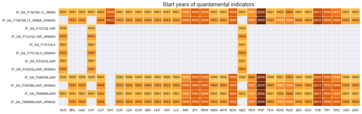
Availability #
It is important to assess data availability before conducting any analysis. It allows identifying any potential gaps or limitations in the dataset, which can impact the validity and reliability of analysis and ensure that a sufficient number of observations for each selected category and cross-section is available as well as determining the appropriate time periods for analysis.
# Availability of industry growth rates

xcatx = [xc for xc in main if xc[:3] == "IP_"]
cidx = cids
msm.check_availability(df, xcats=xcatx, cids=cidx, missing_recent=False)
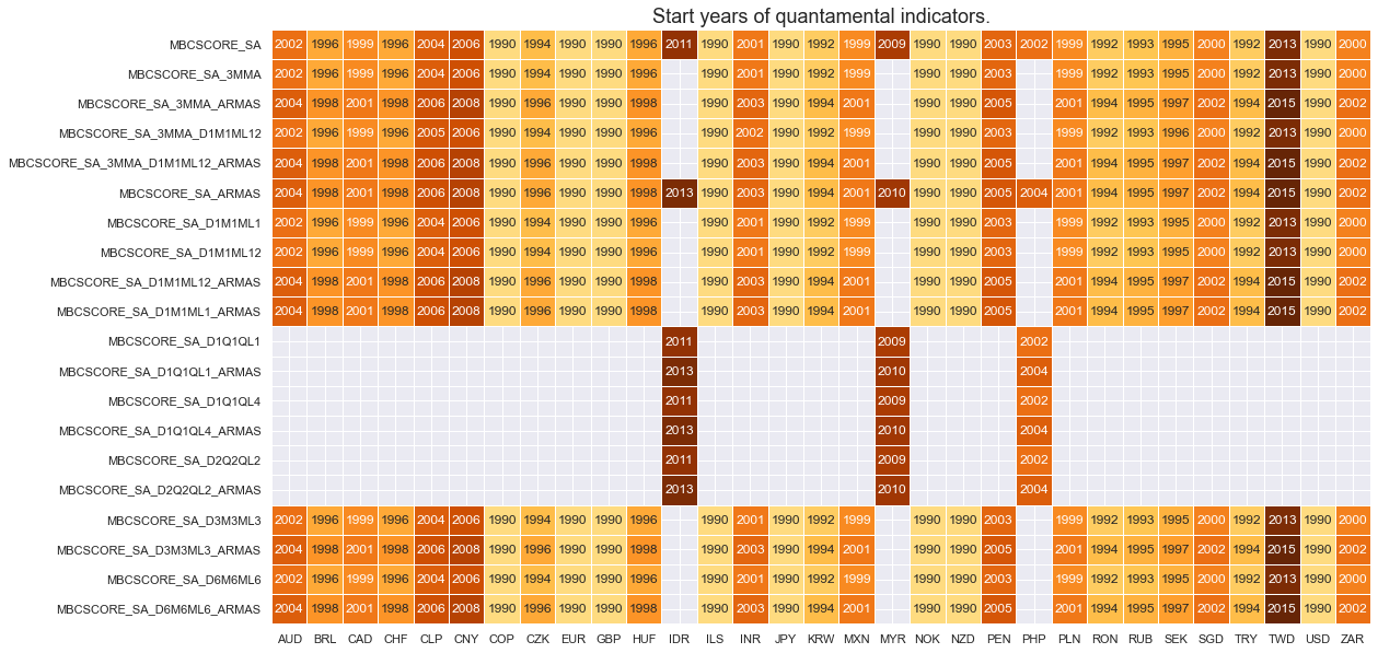
# Availability of manufacturing survey scores

xcatx = [xc for xc in main if xc[:3] == "MBC"]
cidx = cids
msm.check_availability(df, xcats=xcatx, cids=cidx, missing_recent=False)
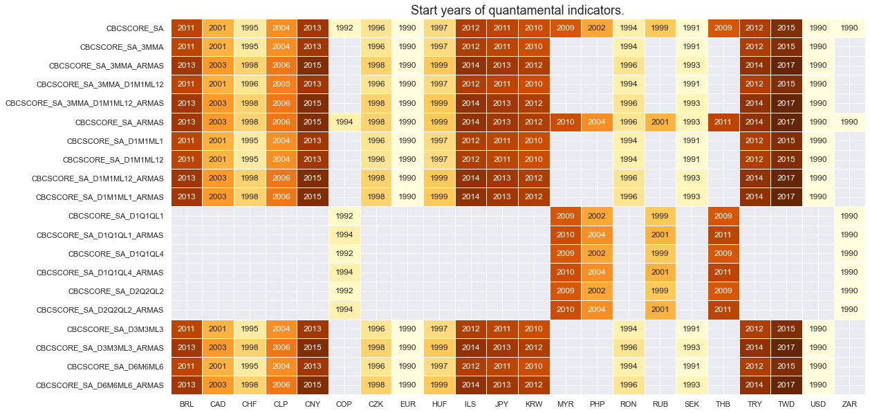
# Availability of construction survey scores

xcatx = [xc for xc in main if xc[:3] == "CBC"]
cidx = cids
msm.check_availability(df, xcats=xcatx, cids=cidx, missing_recent=False)
xcatx = mark
cidx = cids_coms

msm.check_availability(dfx, xcats=xcatx, cids=cidx, missing_recent=False)

Transformations and checks #
Renaming of quarterly tickers #
df_tickers = msm.reduce_df(dfx, xcats=main).groupby(["cid", "xcat"], as_index=False)["value"].count()
df_tickers["ticker"] = df_tickers["cid"] + "_" + df_tickers["xcat"]

df_tickers["transformation"] = df_tickers["xcat"].str.split("_").map(lambda x: x[2] if len(x) > 2 else None)
df_tickers["frequency"] = df_tickers["transformation"].map(lambda x: x[2] if isinstance(x, str) else None)
df_tickers["cx"] = df_tickers["cid"] + "_" + df_tickers["xcat"].str.split("_", n=1).map(lambda x: x[0])

group = df_tickers.groupby(["cx", "frequency"], as_index=False)["xcat"].count()

freq_num_map = {"M": 1, "Q": 3}
group["freq_num"] = group["frequency"].map(freq_num_map)

group_freq_num = group.groupby(["cx"], as_index=False)["freq_num"].max()
freq_num_map_inv = {v: k for k, v in freq_num_map.items()}
group_freq_num["frequency"] = group_freq_num["freq_num"].map(freq_num_map_inv)
group_freq_num.sort_values(by=["cx"])
mask = group_freq_num["frequency"] == "Q"
dict_freq = {
    "Q": group_freq_num.loc[mask, "cx"].values.tolist(),
    "M": group_freq_num.loc[~mask, "cx"].values.tolist(),
}
dict_repl = {
    # Industrial Product trends: Forecasts and Revision Surprises
    "IP_SA_P1Q1QL1AR_ARMAS": "IP_SA_P3M3ML3AR_ARMAS",
    "IP_SA_P2Q2QL2AR_ARMAS": "IP_SA_P6M6ML6AR_ARMAS",
    "IP_SA_P1Q1QL4_ARMAS": "IP_SA_P1M1ML12_3MMA_ARMAS",
    # Manufacturing Confidence Scores
    "MBCSCORE_SA_D1Q1QL1": "MBCSCORE_SA_D3M3ML3",
    "MBCSCORE_SA_D2Q2QL2": "MBCSCORE_SA_D6M6ML6",
    "MBCSCORE_SA_D1Q1QL4": "MBCSCORE_SA_3MMA_D1M1ML12",
    # Forecast and Revision Surprises
    "MBCSCORE_SA_D1Q1QL1_ARMAS": "MBCSCORE_SA_D3M3ML3_ARMAS",
    "MBCSCORE_SA_D2Q2QL2_ARMAS": "MBCSCORE_SA_D6M6ML6_ARMAS",
    "MBCSCORE_SA_D1Q1QL4_ARMAS": "MBCSCORE_SA_3MMA_D1M1ML12_ARMAS",
    # Construction Confidence Scores
    "CBCSCORE_SA_D1Q1QL1": "CBCSCORE_SA_D3M3ML3",
    "CBCSCORE_SA_D2Q2QL2": "CBCSCORE_SA_D6M6ML6",
    "CBCSCORE_SA_D1Q1QL4": "CBCSCORE_SA_3MMA_D1M1ML12",
    # Surprises ARMA(1,1) (ARMAS)
    "CBCSCORE_SA_D1Q1QL1_ARMAS": "CBCSCORE_SA_D3M3ML3_ARMAS",
    "CBCSCORE_SA_D2Q2QL2_ARMAS": "CBCSCORE_SA_D6M6ML6_ARMAS",
    "CBCSCORE_SA_D1Q1QL4_ARMAS": "CBCSCORE_SA_3MMA_D1M1ML12_ARMAS",
}

for key, value in dict_repl.items():
    dfx["xcat"] = dfx["xcat"].str.replace(key, value)

dfx = dfx.sort_values(["cid", "xcat", "real_date"])
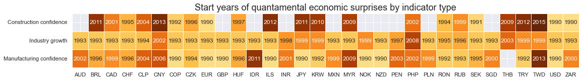
# Simplified availability graph
cidx = cids

dict_names = {
    "IP_SA_P1M1ML12_3MMA_ARMAS": "Industry growth",
    "MBCSCORE_SA": "Manufacturing confidence",
    "CBCSCORE_SA": "Construction confidence",
}
dfxx = msm.reduce_df(dfx, xcats=list(dict_names.keys()), cids=cidx)


for key, value in dict_names.items():
    dfxx["xcat"] = dfxx["xcat"].str.replace(key, value)

msm.check_availability(
    dfxx,
    xcats=list(dict_names.values()),
    cids=cidx,
    missing_recent=False,
    title="Start years of quantamental economic surprises by indicator type",
    start_size=(18, 2),
)
# Cross-sections available for each category group
cids_ips = list(dfx.loc[dfx['xcat'].isin(ips), 'cid'].unique())
cids_mcs = list(dfx.loc[dfx['xcat'].isin(mcs), 'cid'].unique())
cids_ccs = list(dfx.loc[dfx['xcat'].isin(ccs), 'cid'].unique())
Normalized information state changes (as benchmarks) #
# Select relevant categories for changes and surprises

inds = [
    "IP_SA_P1M1ML12_3MMA",
    "IP_SA_P6M6ML6AR",
    "IP_SA_P3M3ML3AR",
    "MBCSCORE_SA",
    "MBCSCORE_SA_D6M6ML6",
    "MBCSCORE_SA_D3M3ML3",
    "CBCSCORE_SA",
    "CBCSCORE_SA_D6M6ML6",
    "CBCSCORE_SA_D3M3ML3",
]
# Normalized and simple information state changes

xcatx = inds
cidx = cids

dfxx = msm.reduce_df(dfx, xcats=xcatx, cids=cidx)

# Create sparse dataframe with information state changes
isc_obj = msm.InformationStateChanges.from_qdf(
    df=dfxx,
    norm=True,  # normalizes changes by first release values
    std="std",
    halflife=36,  # for volatility scaling only
    min_periods=36,
    score_by="diff",
)

dfa = isc_obj.to_qdf(value_column="zscore", postfix="_NIC", thresh=3)
basic_cols = ["real_date", "cid", "xcat", "value"]
dfx = msm.update_df(dfx, dfa[basic_cols])

# Get the changes (without normalisation)
dfa = isc_obj.to_qdf(value_column="diff", postfix="_IC")
dfx = msm.update_df(dfx, dfa[basic_cols])
# Transform to units of annualized information state changes

xcatx = [xc + "_NIC" for xc in inds]
dfa = msm.reduce_df(dfx, xcats=xcatx)

dfa["cx"] = dfa["cid"] + "_" + dfa["xcat"].str.split("_").map(lambda x: x[0])
filt_q = dfa["cx"].isin(dict_freq["Q"])

# Categories with monthly and quarterly releases
dfa.loc[filt_q, "value"] *= np.sqrt(1/4)
dfa.loc[~filt_q, "value"] *= np.sqrt(1/12)

# New names
dfa["xcat"] += "A"
dfa.drop(["cx"], axis=1)

dfx = msm.update_df(dfx, dfa)
Normalized ARMA surprises #
# Normalized ARMA surprises

inds_armas = [xc + "_ARMAS" for xc in inds]
xcatx = inds_armas
cidx = cids

dfxx = msm.reduce_df(dfx, xcats=xcatx, cids=cidx)

# creates sparse dataframe with information state changes
isc_obj = msm.InformationStateChanges.from_qdf(
    df=dfxx,
    norm=True,  # normalizes changes by first release values
    std="std",
    halflife=36,  # for volatility scaling only
    min_periods=36,
    score_by="level",
)

dfa = isc_obj.to_qdf(value_column="zscore", postfix="N", thresh=3)
dfx = msm.update_df(dfx, dfa[basic_cols])
# Transform to units of normalized winsorized surprises in annualized units

xcatx = [xc + "N" for xc in inds_armas]
dfa = msm.reduce_df(dfx, xcats=xcatx)

dfa["cx"] = dfa["cid"] + "_" + dfa["xcat"].str.split("_").map(lambda x: x[0])
filt_q = dfa["cx"].isin(dict_freq["Q"])

# Categories with monthly and quarterly releases
dfa.loc[filt_q, "value"] *= np.sqrt(1/4)
dfa.loc[~filt_q, "value"] *= np.sqrt(1/12)

# New names
dfa["xcat"] += "A"
dfa.drop(["cx"], axis=1)

dfx = msm.update_df(dfx, dfa)
Checkup charts #
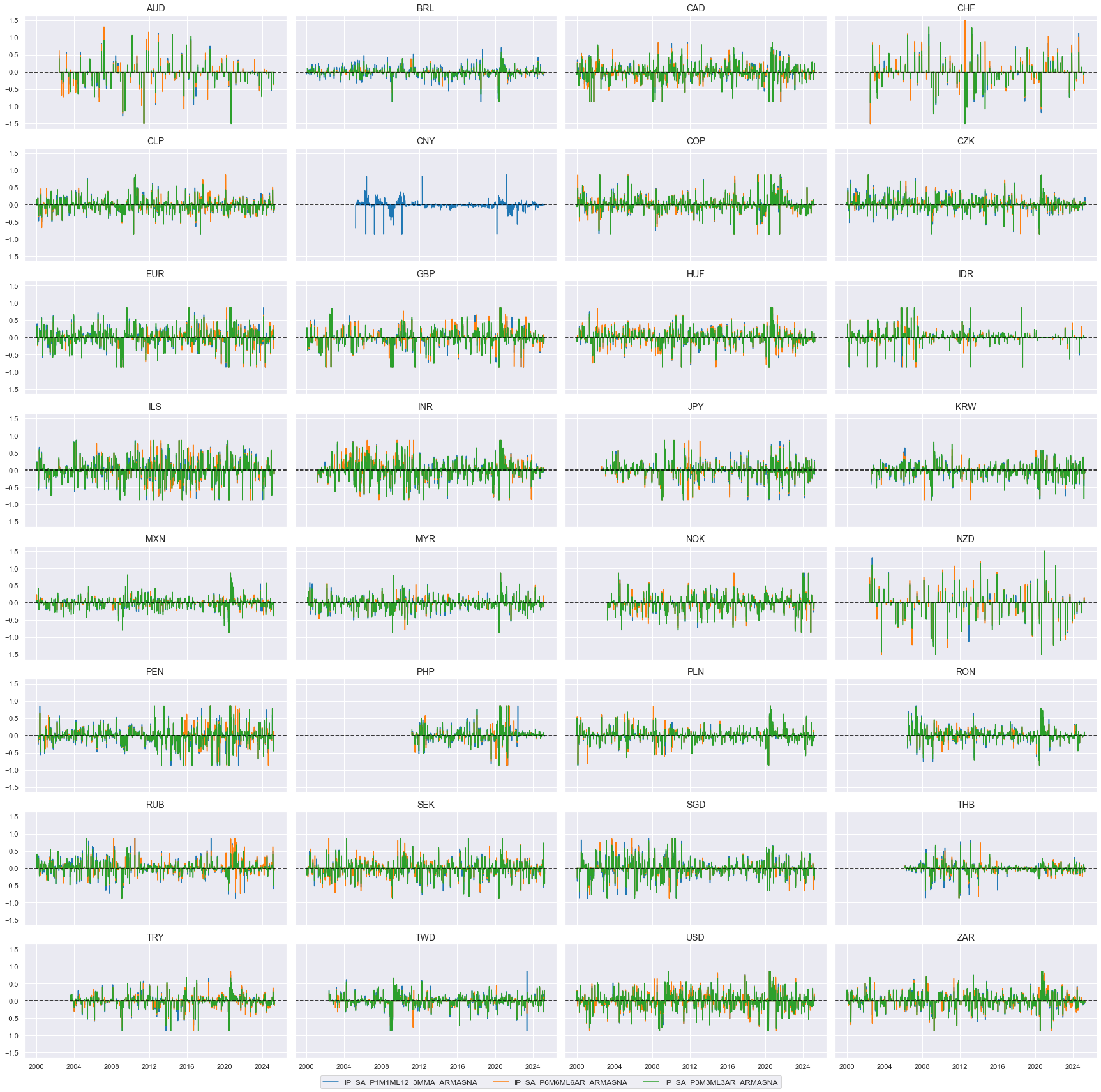
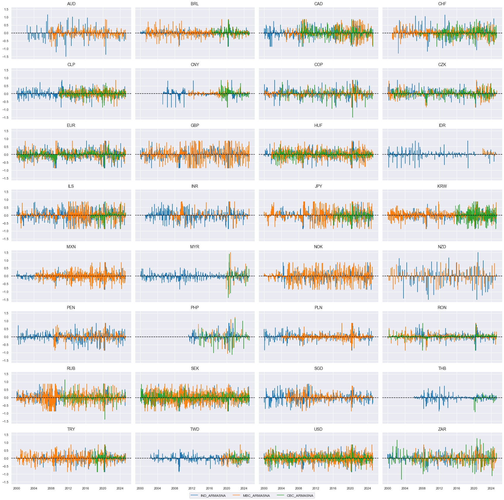
Normalized winsorized and annualized surprises by economic report type #
nwa_surprises = [xc + "NA" for xc in inds_armas]
nwa_surprises_ind = [ns for ns in nwa_surprises if ns[:3] == "IP_"]
nwa_surprises_mbc = [ns for ns in nwa_surprises if ns[:3] == "MBC"]
nwa_surprises_cbc = [ns for ns in nwa_surprises if ns[:3] == "CBC"]

nwa_changes = [xc + "_NICA" for xc in inds]
nwa_changes_ind = [ns for ns in nwa_changes if ns[:3] == "IP_"]
nwa_changes_mbc = [ns for ns in nwa_changes if ns[:3] == "MBC"]
nwa_changes_cbc = [ns for ns in nwa_changes if ns[:3] == "CBC"]
xcatx = nwa_surprises_ind
cidx = list(dfx.loc[dfx['xcat'].isin(xcatx), 'cid'].unique())

msp.view_timelines(
    dfx,
    xcats=xcatx,
    cids=cidx,
    ncol=4,
    start="2000-01-01",
    title=None,
    same_y=True,
    height=2,
    aspect = 2,
)
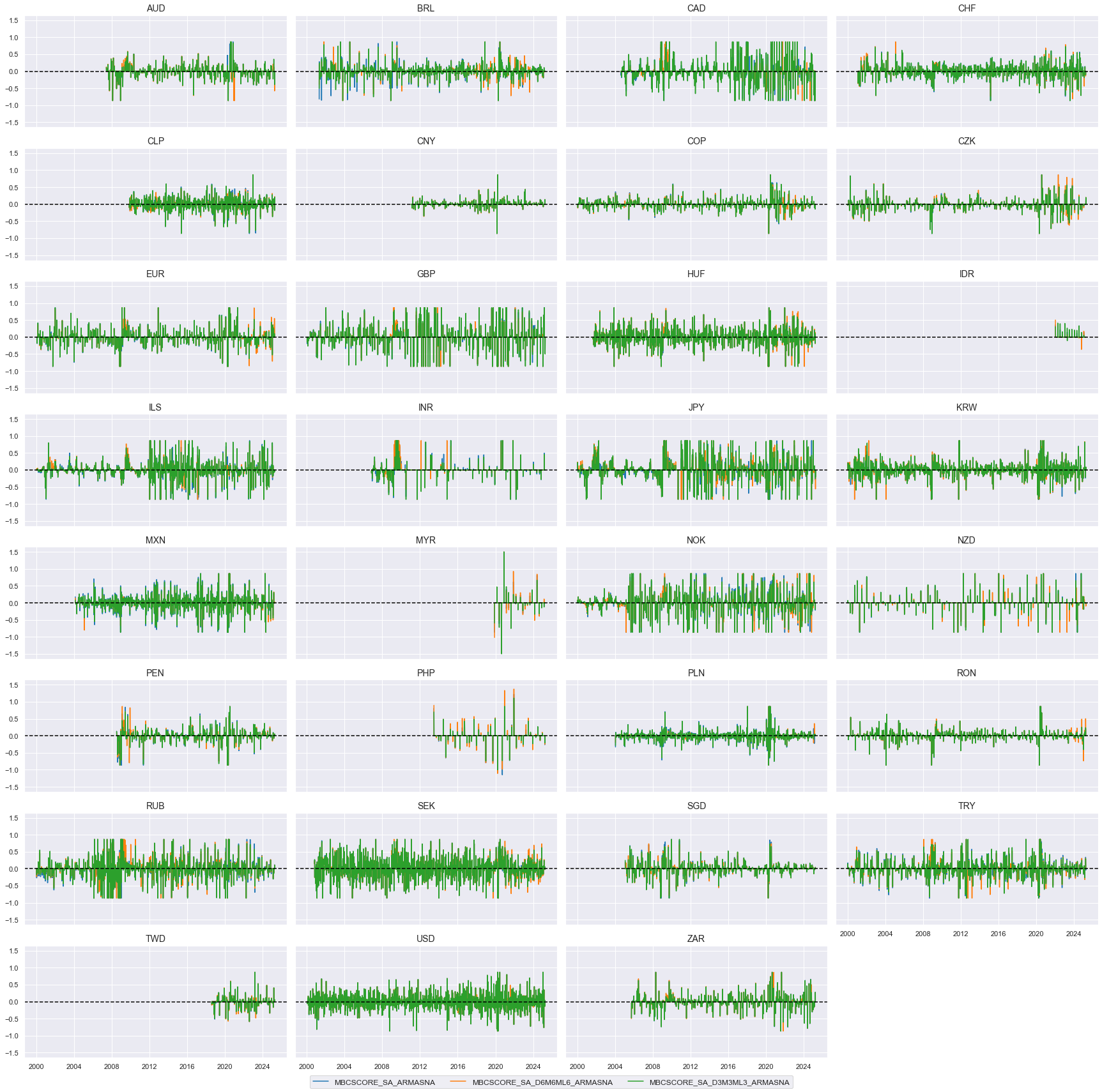
xcatx = nwa_surprises_mbc
cidx = list(dfx.loc[dfx['xcat'].isin(xcatx), 'cid'].unique())

msp.view_timelines(
    dfx,
    xcats=xcatx,
    cids=cidx,
    ncol=4,
    start="2000-01-01",
    title=None,
    same_y=True,
    height=2,
    aspect = 2,
)
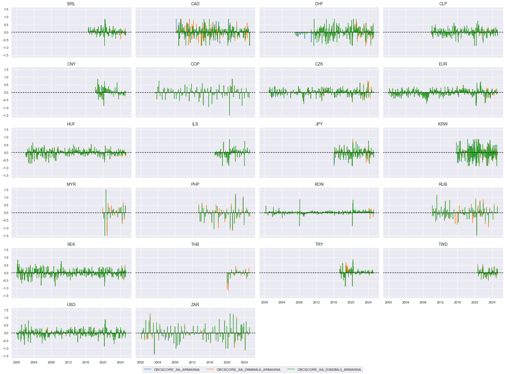
xcatx = nwa_surprises_cbc
cidx = list(dfx.loc[dfx['xcat'].isin(xcatx), 'cid'].unique())

msp.view_timelines(
    dfx,
    xcats=xcatx,
    cids=cidx,
    ncol=4,
    start="2000-01-01",
    title=None,
    same_y=True,
    height=2,
    aspect = 2,
)
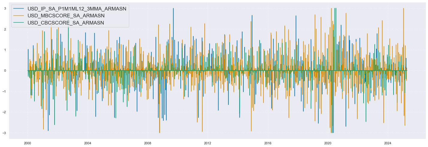
xcatx = ["IP_SA_P1M1ML12_3MMA_ARMASN", "MBCSCORE_SA_ARMASN", "CBCSCORE_SA_ARMASN"]
cidx = ["USD"]

msp.view_timelines(
    dfx,
    xcats=xcatx,
    cids=cidx,
    # start="2015-01-01",
    # end="2025-12-31",
    # title="Industrial production trends, seasonally-adjusted, 3-month over 3-month, annualized rates",
    title_adj=1.02,
    title_xadj=0.435,
    title_fontsize=27,
    legend_fontsize=17,
    size=(20, 7),
)
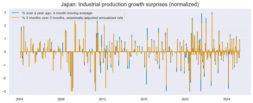
xcatx = ["IP_SA_P1M1ML12_3MMA_ARMASN", "IP_SA_P3M3ML3AR_ARMASN"]
cidx = ["JPY"]

msp.view_timelines(
    dfx,
    xcats=xcatx,
    cids=cidx,
    start="2004-01-01",
    title="Japan: Industrial production growth surprises (normalized)",
    xcat_labels=[
        "% over a year ago, 3-month moving average",
        "% 3 months over 3 months, seasonally-adjusted annualized rate",
    ],
    size=(12, 5),
)
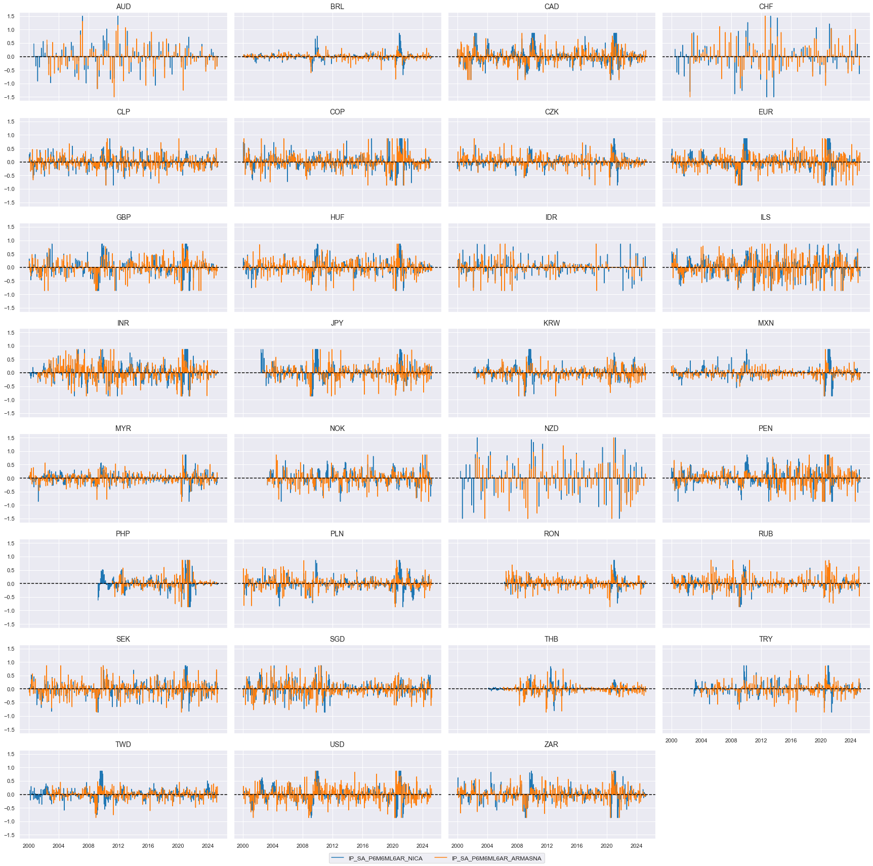
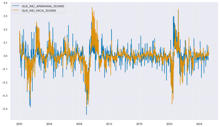
Surprises versus information state changes #
# 'IP_SA_P1M1ML12_3MMA', 'IP_SA_P6M6ML6AR', 'IP_SA_P3M3ML3AR',
# 'MBCSCORE_SA', 'MBCSCORE_SA_D6M6ML6', 'MBCSCORE_SA_D3M3ML3',
# 'CBCSCORE_SA', 'CBCSCORE_SA_D6M6ML6', 'CBCSCORE_SA_D3M3ML3'

xc = "IP_SA_P6M6ML6AR"
xcatx = [xc + "_NICA", xc + "_ARMASNA"]
cidx = list(dfx.loc[dfx['xcat'].isin(xcatx), 'cid'].unique())

msp.view_timelines(
    dfx,
    xcats=xcatx,
    cids=cidx,
    ncol=4,
    start="2000-01-01",
    title=None,
    same_y=True,
    height=2,
    aspect = 2,
)
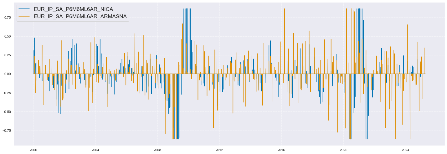
xc = "IP_SA_P6M6ML6AR"
xcatx = [xc + "_NICA", xc + "_ARMASNA"]
cidx = ["EUR"]

msp.view_timelines(
    dfx,
    xcats=xcatx,
    cids=cidx,
    # start="2015-01-01",
    # end="2025-12-31",
    # title="Industrial production trends, seasonally-adjusted, 3-month over 3-month, annualized rates",
    title_adj=1.02,
    title_xadj=0.435,
    title_fontsize=27,
    legend_fontsize=17,
    size=(20, 7),
)
Example strategy: global metals futures #
Signal generation #
Composite surprises (and information state changes) #
# Linear composites of surprises

cidx = cids

dict_surprises = {
    "IND": nwa_surprises_ind,
    "MBC": nwa_surprises_mbc,
    "CBC": nwa_surprises_cbc,
}

dfa = pd.DataFrame(columns=list(dfx.columns))
for key, value in dict_surprises.items():
    dfaa = msp.linear_composite(dfx, xcats=value, cids=cidx, new_xcat=f"{key}_ARMASNA")
    dfa = msm.update_df(dfa, dfaa)

dfx = msm.update_df(dfx, dfa)
comp_surprises = [f"{key}_ARMASNA" for key in dict_surprises.keys()]
# Linear composites of changes

cidx = cids

dict_changes = {
    "IND": nwa_changes_ind,
    "MBC": nwa_changes_mbc,
    "CBC": nwa_changes_cbc,
}

dfa = pd.DataFrame(columns=list(dfx.columns))
for key, value in dict_changes.items():
    dfaa = msp.linear_composite(dfx, xcats=value, cids=cidx, new_xcat=f"{key}_NICA")
    dfa = msm.update_df(dfa, dfaa)

dfx = msm.update_df(dfx, dfa)
comp_changes = [f"{key}_NICA" for key in dict_changes.keys()]
xcatx = comp_surprises  # comp_changes
cidx = list(dfx.loc[dfx['xcat'].isin(xcatx), 'cid'].unique())

msp.view_timelines(
    dfx,
    xcats=xcatx,
    cids=cidx,
    ncol=4,
    start="2000-01-01",
    title=None,
    same_y=True,
    height=2,
    aspect = 2,
)
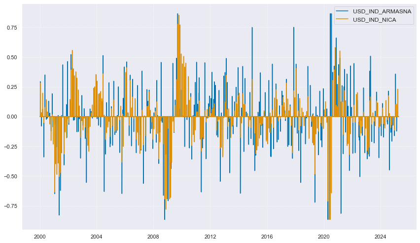
xcatx = ["IND_ARMASNA", "IND_NICA"]
cidx = ["USD"]

msp.view_timelines(
    dfx,
    xcats=xcatx,
    cids=cidx,
    ncol=4,
    start="2000-01-01",
    title=None,
    same_y=True,
    height=2,
    aspect = 2,
)
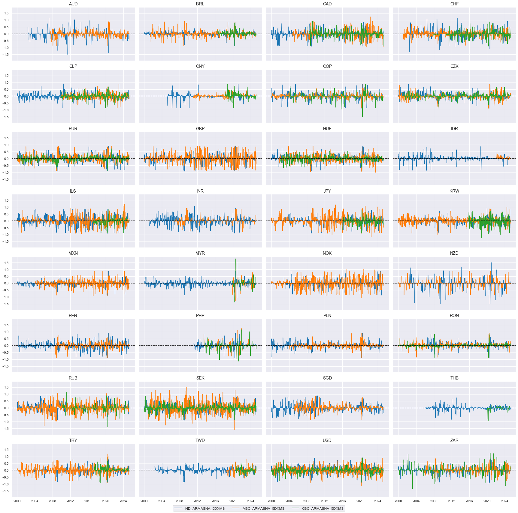
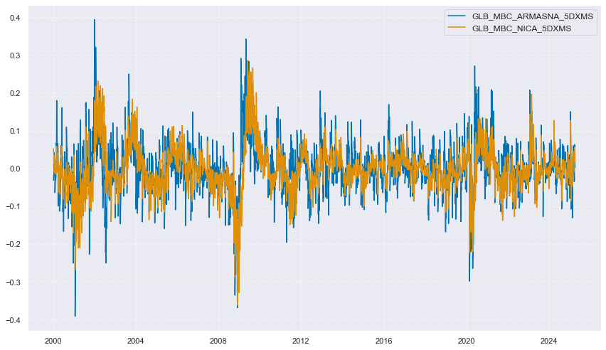
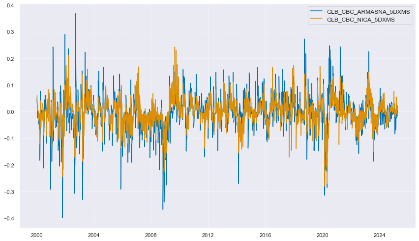
Moving sums #
# 3-day and 5-day moving sums of changes and surprises

xcatx = comp_changes + comp_surprises
cidx = cids
hts = [5, 3]  # Half-times

dfa = msm.reduce_df(dfx, xcats=xcatx, cids=cidx)
dfa["ticker"] = dfa["cid"] + "_" + dfa["xcat"]
p = dfa.pivot(index="real_date", columns="ticker", values="value")

store = []
for ht in hts:
    proll = p.ewm(halflife=ht).sum()
    proll.columns += f"_{ht}DXMS"
    _df = proll.stack().to_frame("value").reset_index()
    _df[["cid", "xcat"]] = _df["ticker"].str.split("_", n=1, expand=True)
    store.append(_df[["cid", "xcat", "real_date", "value"]])

dfx = msm.update_df(dfx, pd.concat(store, axis=0, ignore_index=True))

comp_changes_3d = [f"{xcat}_3DXMS" for xcat in comp_changes]
comp_changes_5d = [f"{xcat}_5DXMS" for xcat in comp_changes]
comp_surprises_3d = [f"{xcat}_3DXMS" for xcat in comp_surprises]
comp_surprises_5d = [f"{xcat}_5DXMS" for xcat in comp_surprises]
xcatx = comp_surprises_5d  # comp_changes_5d
cidx = list(dfx.loc[dfx['xcat'].isin(xcatx), 'cid'].unique())

msp.view_timelines(
    dfx,
    xcats=xcatx,
    cids=cidx,
    ncol=4,
    start="2000-01-01",
    title=None,
    same_y=True,
    height=2,
    aspect = 2,
)
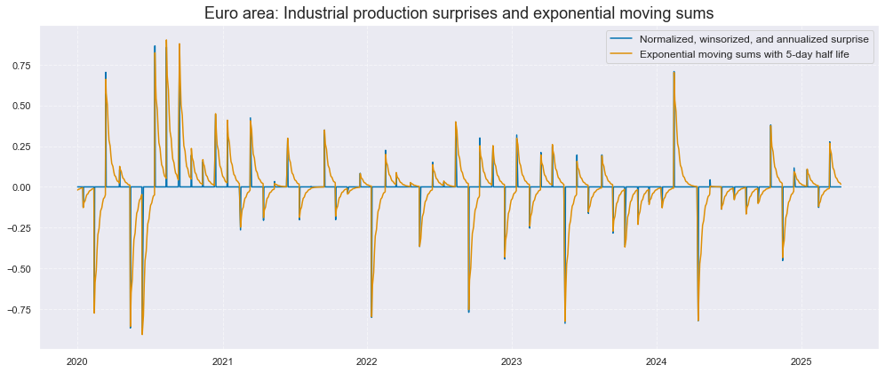
xc = "IND"
xcatx = [xc + "_ARMASNA", xc + "_ARMASNA_5DXMS"]
cidx = ["EUR"]

msp.view_timelines(
    dfx,
    xcats=xcatx,
    cids=cidx,
    start="2020-01-01",
    title="Euro area: Industrial production surprises and exponential moving sums",
    xcat_labels=[
        "Normalized, winsorized, and annualized surprise",
        "Exponential moving sums with 5-day half life",
    ],
    size=(14, 6),
)
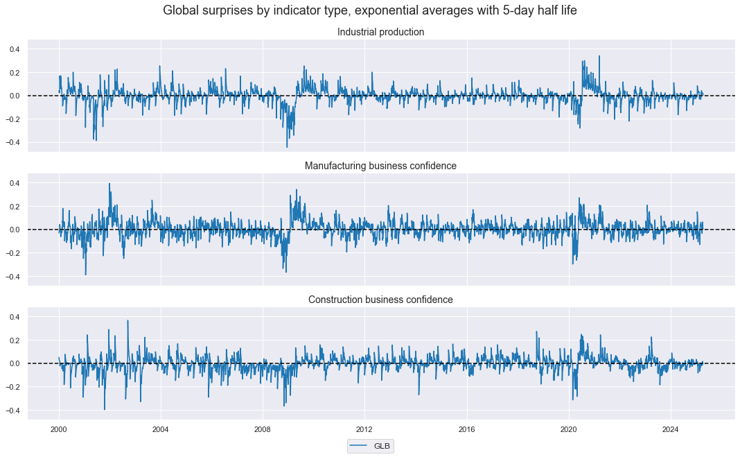
Global surprises by report type #
# Create global IP-weighted changes and surprises

xcatx = comp_changes_3d + comp_changes_5d + comp_surprises_3d + comp_surprises_5d

store = []
for xc in xcatx:
    dfr = msm.reduce_df(dfx, cids=cids, xcats=[xc, "IVAWGT_SA_1YMA"])
    dfa = msp.linear_composite(
        df=dfr,
        xcats=xc,
        cids=cids,
        weights="IVAWGT_SA_1YMA",
        new_cid="GLB",
        complete_cids=False,
    )
    store.append(dfa)
dfx = msm.update_df(dfx, pd.concat(store, axis=0))
cidx = ["GLB"]

for cat in ("IND", "MBC", "CBC"):
    xcatx = [xc for xc in comp_surprises_5d + comp_changes_5d if xc.startswith(cat)]  # comp_changes_3d, comp_changes_5d, comp_surprises_3d, comp_surprises_5d
    msp.view_timelines(
        dfx,
        xcats=xcatx,
        # xcat_grid=True,
        cids=cidx,
        ncol=1,
        start="2000-01-01",
        title=None,
        same_y=True,
        height=2.5,
        aspect = 5,
    )
xcatx = comp_surprises_5d  # comp_changes_3d, comp_changes_5d, comp_surprises_3d, comp_surprises_5d
cidx = ["GLB"]

msp.view_timelines(
    dfx,
    xcats=xcatx,
    xcat_grid=True,
    cids=cidx,
    ncol=1,
    start="2000-01-01",
    title="Global surprises by indicator type, exponential averages with 5-day half life",
    xcat_labels=["Industrial production", "Manufacturing business confidence", "Construction business confidence"],
    same_y=True,
    height=2,
    aspect = 5,
)
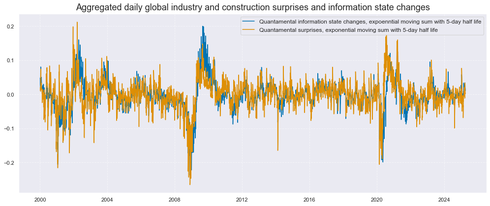
Global aggregate surprises and changes #
cidx = ["GLB"]
dict_aggs = {
    "ARMASNA_3DXMS": comp_surprises_3d,
    "ARMASNA_5DXMS": comp_surprises_5d,
    "NICA_3DXMS": comp_changes_3d,
    "NICA_5DXMS": comp_changes_5d,
}

dfa = pd.DataFrame(columns=list(dfx.columns))
for key, value in dict_aggs.items():
    dfaa = msp.linear_composite(dfx, xcats=value, cids=cidx, new_xcat=key)
    dfa = msm.update_df(dfa, dfaa)

dfx = msm.update_df(dfx, dfa)

gascs = [key for key in dict_aggs.keys()]
xcatx = ["NICA_5DXMS", "ARMASNA_5DXMS"]
cidx = ["GLB"]

msp.view_timelines(
    dfx,
    xcats=xcatx,
    cids=cidx,
    start="2000-01-01",
    title="Aggregated daily global industry and construction surprises and information state changes",
    xcat_labels=[
        "Quantamental information state changes, expoenntial moving sum with 5-day half life",
        "Quantamental surprises, exponential moving sum with 5-day half life",
    ],
    size=(14, 6),
)
Global commodity basket target returns #
# Target of commodity basket
cids_co = cids_coms
cts = [cid + "_" for cid in cids_co]
bask_co = msp.Basket(dfx, contracts=cts, ret="COXR_VT10")
bask_co.make_basket(weight_meth="equal", basket_name="GLB")
dfa = bask_co.return_basket()

dfx = msm.update_df(dfx, dfa)
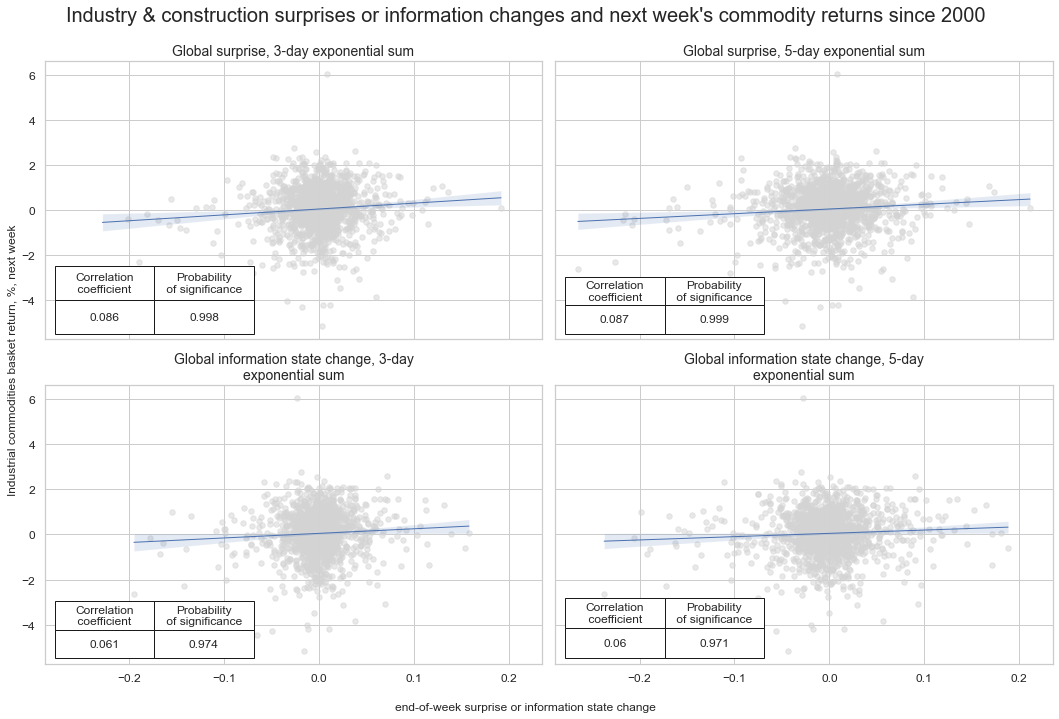
Value checks #
Specs and panel test #
dict_local = {
    "sigs": gascs,
    "targs": ["COXR_VT10"],
    "cidx": ["GLB"],
    "start": "2000-01-01",
    "black": None,
    "srr": None,
    "pnls": None,
}
dix = dict_local

sigs = dix["sigs"]
targ = dix["targs"][0]
cidx = dix["cidx"]
blax = dix["black"]
start = dix["start"]

# Initialize the dictionary to store CategoryRelations instances

dict_cr = {}

for sig in sigs:
    dict_cr[sig] = msp.CategoryRelations(
        dfx,
        xcats=[sig, targ],
        cids=cidx,
        freq="W",
        lag=1,
        xcat_aggs=["last", "sum"],
        start=start,
    )
# Plotting the results

crs = list(dict_cr.values())
crs_keys = list(dict_cr.keys())
ncol = 2 if len(dict_cr) % 2 == 0 else 3
nrow = np.ceil(len(dict_cr) / 2)

msv.multiple_reg_scatter(
    cat_rels=crs,
    # title="Macroeconomic information state changes and subsequent weekly duration returns, 22 countries, since 2000",
    # ylab="5-year IRS fixed receiver returns, %, vol-targeted position at 10% ar, next week",
    ncol=2,
    nrow=2,
    figsize=(15, 10),
    prob_est="pool",  # No panel to operate on so direct pearson correlation and significance.
    coef_box="lower left",
    title="Industry & construction surprises or information changes and next week's commodity returns since 2000",
    subplot_titles=["Global surprise, 3-day exponential sum",
                    "Global surprise, 5-day exponential sum",
                    "Global information state change, 3-day exponential sum",
                    "Global information state change, 5-day exponential sum"],
    xlab="end-of-week surprise or information state change",
    ylab="Industrial commodities basket return, %, next week",
)
Accuracy and correlation check #
dix = dict_local

sigx = dix["sigs"]
targx = [dix["targs"][0]]
cidx = dix["cidx"]
start = dix["start"]
blax = dix["black"]

srr = mss.SignalReturnRelations(
    dfx,
    cids=cidx,
    sigs=sigx,
    rets=targx,
    sig_neg=[False] * len(sigx),
    freqs="D",
    start=start,
    blacklist=blax,
)

dix["srr"] = srr
dix = dict_local
srr = dix["srr"]
display(srr.multiple_relations_table().astype("float").round(3))
| accuracy | bal_accuracy | pos_sigr | pos_retr | pos_prec | neg_prec | pearson | pearson_pval | kendall | kendall_pval | auc | ||||
|---|---|---|---|---|---|---|---|---|---|---|---|---|---|---|
| Return | Signal | Frequency | Aggregation | |||||||||||
| COXR_VT10 | ARMASNA_3DXMS | D | last | 0.514 | 0.514 | 0.498 | 0.526 | 0.540 | 0.488 | 0.050 | 0.000 | 0.025 | 0.002 | 0.514 |
| ARMASNA_5DXMS | D | last | 0.513 | 0.513 | 0.487 | 0.526 | 0.540 | 0.487 | 0.050 | 0.000 | 0.027 | 0.001 | 0.514 | |
| NICA_3DXMS | D | last | 0.508 | 0.510 | 0.455 | 0.526 | 0.537 | 0.484 | 0.046 | 0.000 | 0.023 | 0.006 | 0.510 | |
| NICA_5DXMS | D | last | 0.504 | 0.507 | 0.445 | 0.526 | 0.534 | 0.480 | 0.041 | 0.001 | 0.021 | 0.010 | 0.507 |
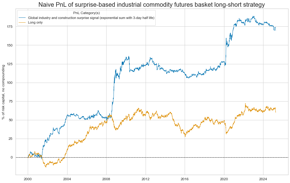
Naive PnL #
dix = dict_local

sigx = dix["sigs"]
targ = dix["targs"][0]
cidx = dix["cidx"]
blax = dix["black"]
start = dix["start"]

dfxx = dfx[["real_date", "cid", "xcat", "value"]]

naive_pnl = msn.NaivePnL(
    dfxx,
    ret=targ,
    sigs=sigx,
    cids=cidx,
    start=start,
    blacklist=blax,
    bms=["USD_EQXR_NSA"],
)

for sig in sigx:
    naive_pnl.make_pnl(
        sig,
        sig_neg=False,
        sig_op="zn_score_cs",
        thresh=3,
        rebal_freq="daily",
        vol_scale=10,
        rebal_slip=0,
        pnl_name=sig + "_PZN",
    )

naive_pnl.make_long_pnl(vol_scale=None, label="Long only")

dix["pnls"] = naive_pnl
dix = dict_local

sigx = dix["sigs"]
start = dix["start"]
cidx = dix["cidx"]
naive_pnl = dix["pnls"]

pnls = [s + "_PZN" for s in sigx[1:2]] + ["Long only"]

naive_pnl.plot_pnls(
    pnl_cats=pnls,
    pnl_cids=["ALL"],
    start=start,
    title="Naive PnL of surprise-based industrial commodity futures basket long-short strategy",
    xcat_labels=[
        "Global industry and construction surprise signal (exponential sum with 3-day half life)",
        "Long only",
    ],
    figsize=(16, 10),
)

display(naive_pnl.evaluate_pnls())
| xcat | ARMASNA_3DXMS_PZN | ARMASNA_5DXMS_PZN | NICA_3DXMS_PZN | NICA_5DXMS_PZN | Long only |
|---|---|---|---|---|---|
| Return % | 6.96169 | 6.71972 | 6.28015 | 5.87504 | 2.401772 |
| St. Dev. % | 10.0 | 10.0 | 10.0 | 10.0 | 7.218695 |
| Sharpe Ratio | 0.696169 | 0.671972 | 0.628015 | 0.587504 | 0.332716 |
| Sortino Ratio | 1.080545 | 1.029082 | 0.971957 | 0.904325 | 0.459871 |
| Max 21-Day Draw % | -17.791954 | -20.143882 | -18.121712 | -18.212939 | -14.302399 |
| Max 6-Month Draw % | -18.407946 | -20.247506 | -20.638582 | -20.48239 | -20.143069 |
| Peak to Trough Draw % | -25.1821 | -29.569912 | -38.672428 | -41.731855 | -38.519882 |
| Top 5% Monthly PnL Share | 0.839176 | 0.876084 | 0.91009 | 1.008755 | 1.166558 |
| USD_EQXR_NSA correl | -0.091936 | -0.100464 | -0.115774 | -0.124091 | 0.291098 |
| Traded Months | 304 | 304 | 304 | 304 | 304 |
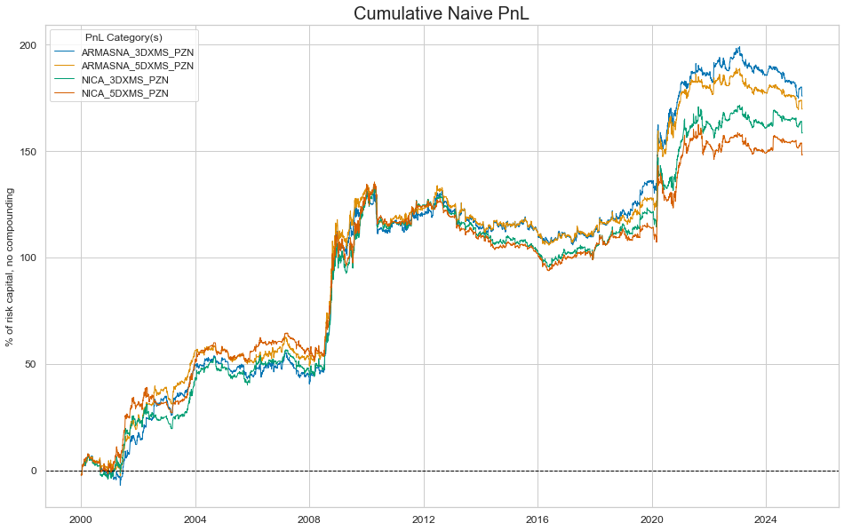
dix = dict_local

sigx = dix["sigs"]
start = dix["start"]
cidx = dix["cidx"]
naive_pnl = dix["pnls"]

pnls = [s + "_PZN" for s in sigx]

naive_pnl.plot_pnls(
    pnl_cats=pnls,
    pnl_cids=["ALL"],
    start=start,
    # title="Naive PnLs of global IRS positions based on macro group information state changes (unbiased signals)",
    # xcat_labels=glabels_ordered[1:],
    figsize=(16, 10),
)
dix = dict_local

sigx = dix["sigs"]
naive_pnl = dix["pnls"]
pnls = [s + "_PZN" for s in sigx]

naive_pnl.signal_heatmap(pnl_name=pnls[0], freq="m", title=None, figsize=(15, 1))