FX forward volatility #
The category group includes basic generic estimates of historic annualized standard deviations of FX forward-returns and related generic leverage measures for 10% annualized volatility targets. Their main purpose in JPMaQS is to facilitate the adjustment of quantamental indicators, factors and returns for volatility across FX forward markets.
Annualized standard deviation of FX forward return #
Ticker : FXXRxEASD_NSA / FXXRUSDxEASD_NSA
Label : Annualized standard deviation of FX forward return: vs. dominant cross / vs. USD.
Definition : Annualized estimated standard deviation of 1-month FX forward return, % of notional, based on exponential moving average of daily returns: vs. dominant cross / vs. USD.
Notes :
-
The standard deviation has been calculated based on an exponential moving average of daily returns with a half-life of 11 active trading days.
-
The default returns are calculated for a contract that is long the local currency of the cross section against its dominant traded benchmark. For most currencies, the benchmark is the dollar. For some European currencies (Switzerland, the Czech Republic, Hungary, Norway, Poland, Romania, Sweden), the benchmark is the euro. For Great Britain, Turkey and Russia, an equally weighted basked of dollars and euros have been used.
-
A separate category for returns against the USD alone has been added for convenience.
-
For the following currencies, returns are based on non-deliverable contracts: IDR, INR, KRW, CNY, MYR and TWD.
-
For some currencies, returns include periods of low liquidity and FX targeting. If one wishes to ‘blacklist’ such periods one should use the non-tradability and FX-target dummies, which have category ticker codes
FXUNTRADABLE_NSAandFXTARGETED_NSA. -
A notable example of such a period is Malaysia in the early 2000s. The statistics in this period are artefacts of the managed exchange rate regime and the data generation process. It is not indicative of the actual exchange rate volatility, hence should be discounted from any analysis.
-
For more information on FX targeting, see the notes for FX tradeability and flexibility .
Annualized standard deviation of FX forward return - Additional tenors #
Ticker : FX03MXRxEASD_NSA / FX06MXRxEASD_NSA / FX09MXRxEASD_NSA / FX01YXRxEASD_NSA
Label : Annualized standard deviation of FX forward return vs. dominant cross: 3m tenor / 6m tenor / 9m tenor / 1y tenor.
Definition : Annualized estimated standard deviation of FX forward return, % of notional, based on exponential moving average of daily returns vs. dominant cross: 3-month forward / 6-month forward / 9-month forward / 1-year forward.
Notes :
-
The standard deviation has been calculated based on an exponential moving average of daily returns with a half-life of 11 active trading days.
-
The default returns are calculated for a contract that is long the local currency of the cross section against its dominant traded benchmark. For most currencies, the benchmark is the dollar. For some European currencies (Switzerland, the Czech Republic, Hungary, Norway, Poland, Romania, Sweden), the benchmark is the euro. For Great Britain, Turkey and Russia, an equally weighted basked of dollars and euros have been used.
-
For the following currencies, returns are based on non-deliverable contracts: IDR, INR, KRW, CNY, MYR and TWD.
-
For some currencies, returns include periods of low liquidity and FX targeting. If one wishes to ‘blacklist’ such periods one should use the non-tradability and FX-target dummies, which have category ticker codes
FXUNTRADABLE_NSAandFXTARGETED_NSA. -
A notable example of such a period is Malaysia in the early 2000s. The statistics in this period are artefacts of the managed exchange rate regime and the data generation process. It is not indicative of the actual exchange rate volatility, hence should be discounted from any analysis.
-
For more information on FX targeting, see the notes for FX tradeability and flexibility .
Leverage ratio of vol-targeted FX forward position #
Ticker : FXXRxLEV10_NSA / FXXRUSDxLEV10_NSA
Label : Leverage ratio of FX forward position for a 10% annualized vol target: based on dominant cross / based on USD.
Definition : FX forward leverage for a 10% annualized vol target, as a ratio of contract notional relative to risk capital on which the return is calculated: based on dominant cross / based on USD.
Notes :
-
This serves as the leverage ratio for a 10% annualized volatility target and is inversely proportional to the estimated annualized standard deviation of the return on a USD 1-month forward notional position.
-
The leverage ratio is capped to 5, in order to avoid excessive leverage in periods of FX pegs or dysfunctional markets.
-
See further the above related notes on “Annualized standard deviation of FX forward return” (
FXXRxEASD_NSA).
Leverage ratio of vol-targeted FX forward position - additional tenors #
Ticker : FX03MXRxLEV10_NSA / FX06MXRxLEV10_NSA / FX09MXRxLEV10_NSA / FX01YXRxLEV10_NSA
Label : Leverage ratio of FX forward position for a 10% annualized vol target based on dominant cross: 3m tenor / 6m tenor / 9m tenor / 1y tenor.
Definition : FX forward leverage for a 10% annualized vol target, as a ratio of contract notional relative to risk capital on which the return is calculated based on dominant cross: 3-month forward / 6-month forward / 9-month forward / 1-year forward.
Notes :
-
This serves as the leverage ratio for a 10% annualized volatility target and is inversely proportional to the estimated annualized standard deviation of the return on a USD 1-month forward notional position.
-
The leverage ratio is capped to 5, in order to avoid excessive leverage in periods of FX pegs or dysfunctional markets.
-
See further the above related notes on “Annualized standard deviation of FX forward return” (
FXXRxEASD_NSA).
Imports #
Only the standard Python data science packages and the specialized
macrosynergy
package are needed.
import os
import pandas as pd

import macrosynergy.management as msm
import macrosynergy.panel as msp
import macrosynergy.visuals as msv
import macrosynergy.signal as mss

from macrosynergy.download import JPMaQSDownload

from timeit import default_timer as timer
from datetime import timedelta, date
import os

import warnings

warnings.simplefilter("ignore")
The
JPMaQS
indicators we consider are downloaded using the J.P. Morgan Dataquery API interface within the
macrosynergy
package. This is done by specifying
ticker strings
, formed by appending an indicator category code
<category>
to a currency area code
<cross_section>
. These constitute the main part of a full quantamental indicator ticker, taking the form
DB(JPMAQS,<cross_section>_<category>,<info>)
, where
<info>
denotes the time series of information for the given cross-section and category. The following types of information are available:
-
valuegiving the latest available values for the indicator -
eop_lagreferring to days elapsed since the end of the observation period -
mop_lagreferring to the number of days elapsed since the mean observation period -
gradedenoting a grade of the observation, giving a metric of real time information quality.
After instantiating the
JPMaQSDownload
class within the
macrosynergy.download
module, one can use the
download(tickers,start_date,metrics)
method to easily download the necessary data, where
tickers
is an array of ticker strings,
start_date
is the first collection date to be considered and
metrics
is an array comprising the times series information to be downloaded.
cids_dmca = [
    "AUD",
    "CAD",
    "CHF",
    "EUR",
    "GBP",
    "JPY",
    "NOK",
    "NZD",
    "SEK",
    "USD",
]  # DM currency areas
cids_dmec = ["DEM", "ESP", "FRF", "ITL", "NLG"]  # DM euro area countries
cids_latm = ["BRL", "COP", "CLP", "MXN", "PEN"]  # Latam countries
cids_emea = ["CZK", "HUF", "ILS", "PLN", "RON", "RUB", "TRY", "ZAR"]  # EMEA countries
cids_emas = [
    "CNY",
    "HKD",
    "IDR",
    "INR",
    "KRW",
    "MYR",
    "PHP",
    "SGD",
    "THB",
    "TWD",
]  # EM Asia countries
cids_dm = cids_dmca + cids_dmec
cids_em = cids_latm + cids_emea + cids_emas
cids = sorted(cids_dm + cids_em)
main = [
    "FXXRxEASD_NSA",
    "FX03MXRxEASD_NSA", "FX06MXRxEASD_NSA", "FX09MXRxEASD_NSA", "FX01YXRxEASD_NSA",
    "FXXRxLEV10_NSA",
    "FX03MXRxLEV10_NSA", "FX06MXRxLEV10_NSA", "FX09MXRxLEV10_NSA", "FX01YXRxLEV10_NSA",
    "FXXRUSDxEASD_NSA",
    "FXXRUSDxLEV10_NSA"
]

mark = ["FXXR_NSA",
        "LCBIR_NSA",
        "FCBIR_NSA",
        "CDS05YXR_NSA",

        "DU10YXRxEASD_NSA",
        "EQXRxEASD_NSA",
        "CDS05YXRxEASD_NSA",
        "EQXRxEASD_NSA",

        "FXTARGETED_NSA",
        "FXUNTRADABLE_NSA",
        ]  # market links


xcats = main + mark
# Download series from J.P. Morgan DataQuery by tickers

start_date = "1990-01-01"
tickers = [cid + "_" + xcat for cid in cids for xcat in xcats]
print(f"Maximum number of tickers is {len(tickers)}")

# Retrieve credentials

client_id: str = os.getenv("DQ_CLIENT_ID")
client_secret: str = os.getenv("DQ_CLIENT_SECRET")

# Download from DataQuery

with JPMaQSDownload(client_id=client_id, client_secret=client_secret) as downloader:
    start = timer()
    assert downloader.check_connection()
    df = downloader.download(
        tickers=tickers,
        start_date=start_date,
        metrics=["value", "eop_lag", "mop_lag", "grading"],
        suppress_warning=True,
    )
    end = timer()


print("Download time from DQ: " + str(timedelta(seconds=end - start)))
Maximum number of tickers is 836
Downloading data from JPMaQS.
Timestamp UTC:  2025-04-03 08:09:44
Connection successful!
Some expressions are missing from the downloaded data. Check logger output for complete list.
724 out of 3192 expressions are missing. To download the catalogue of all available expressions and filter the unavailable expressions, set `get_catalogue=True` in the call to `JPMaQSDownload.download()`.
Download time from DQ: 0:01:54.573538
Availability #
cids_exp = sorted(
    list(set(cids) - set(cids_dmec + ["HKD", "USD"]))
)  # cids expected in category panels
msm.missing_in_df(df, xcats=main, cids=cids_exp)
No missing XCATs across DataFrame.
Missing cids for FX01YXRxEASD_NSA:   []
Missing cids for FX01YXRxLEV10_NSA:  []
Missing cids for FX03MXRxEASD_NSA:   []
Missing cids for FX03MXRxLEV10_NSA:  []
Missing cids for FX06MXRxEASD_NSA:   []
Missing cids for FX06MXRxLEV10_NSA:  []
Missing cids for FX09MXRxEASD_NSA:   []
Missing cids for FX09MXRxLEV10_NSA:  []
Missing cids for FXXRUSDxEASD_NSA:   []
Missing cids for FXXRUSDxLEV10_NSA:  []
Missing cids for FXXRxEASD_NSA:      []
Missing cids for FXXRxLEV10_NSA:     []
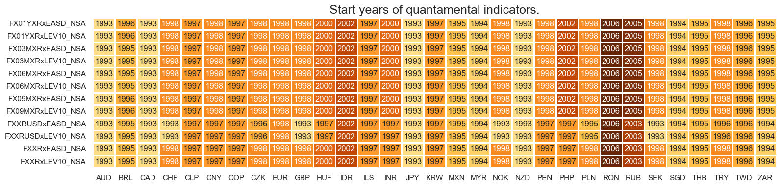
Quantamental indicators for FX forward volatility are available from 2000 for most currency areas. The notable exceptions are Indonesia, Romania and Russia.
For the explanation of currency symbols, which are related to currency areas or countries for which categories are available, please view Appendix 1 .
xcatx = main
cidx = cids_exp

dfx = msm.reduce_df(df, xcats=xcatx, cids=cidx)
dfs = msm.check_startyears(
    dfx,
)
msm.visual_paneldates(dfs, size=(18, 4))

print("Last updated:", date.today())
Last updated: 2025-04-03
History #
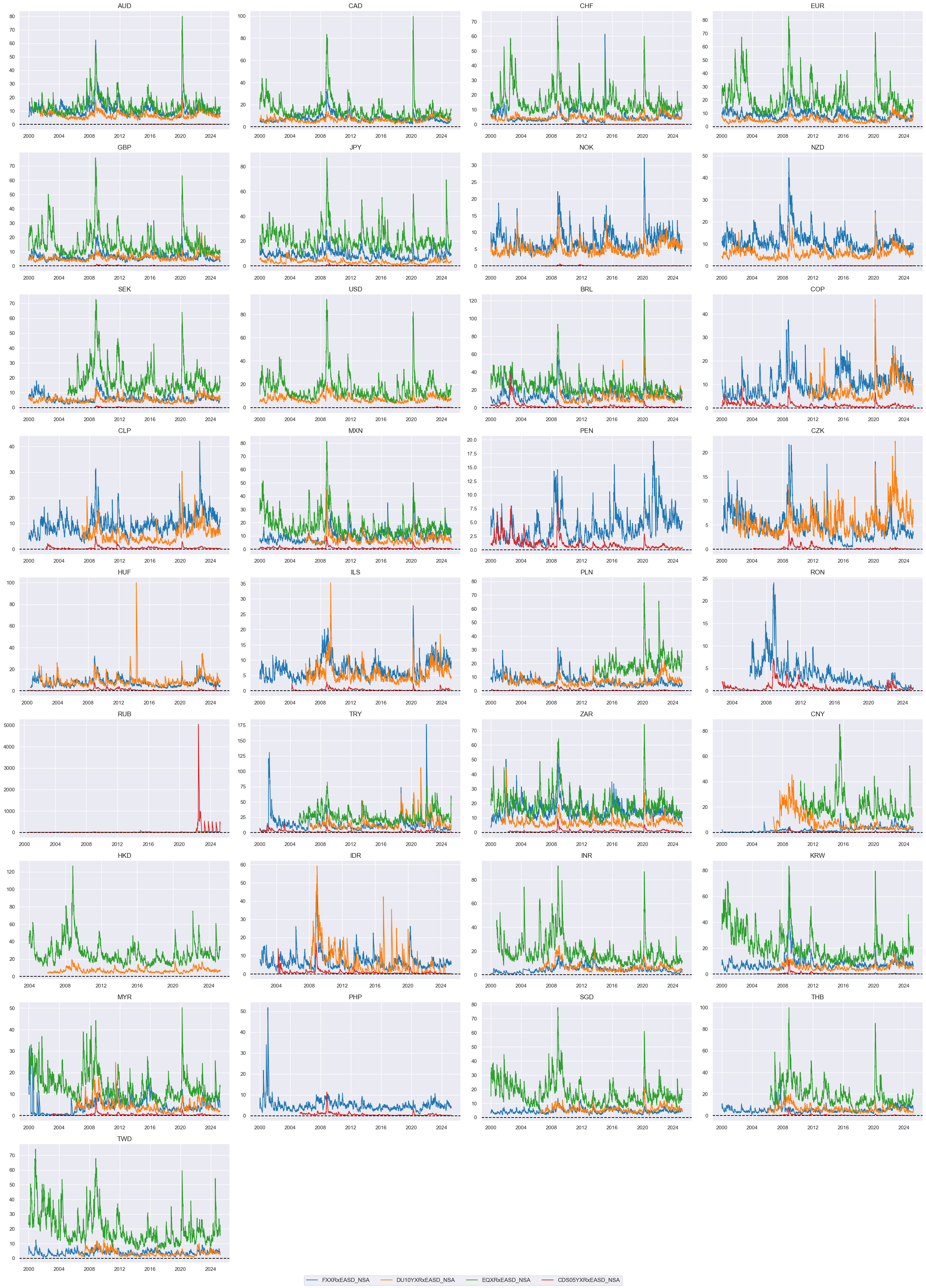
Annualized standard deviations of FX forward return #
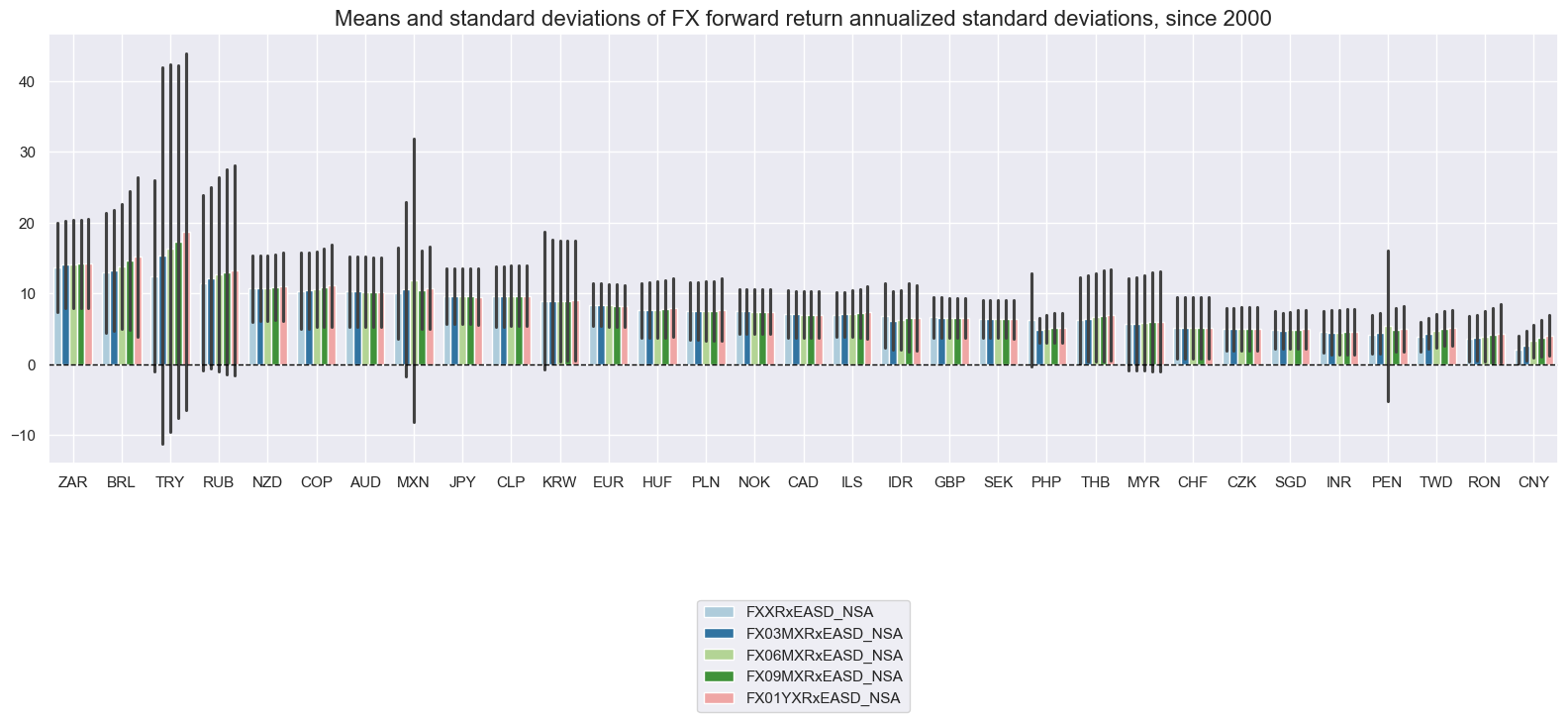
Across countries, average annualized standard deviations have ranged from under 5% to close to 20%. FX return variations was lowest for currencies with a high degree of exchange rate management by the central bank. Standard deviations have been quite diverse and time variant. RUB and TRY have exceeded 100% annualized volatility in past episodes.
xcatx = [
    "FXXRxEASD_NSA", "FX03MXRxEASD_NSA", "FX06MXRxEASD_NSA", "FX09MXRxEASD_NSA", "FX01YXRxEASD_NSA",
]
cidx = cids_exp

msp.view_ranges(
    df,
    xcats=xcatx,
    cids=cidx,
    sort_cids_by="mean",
    start=start_date,
    kind="bar",
    title="Means and standard deviations of FX forward return annualized standard deviations, since 2000",

    size=(16, 8),
)
xcatx = [
    "FXXRxEASD_NSA", "FX03MXRxEASD_NSA", "FX06MXRxEASD_NSA", "FX09MXRxEASD_NSA", "FX01YXRxEASD_NSA",
]
cidx = cids_exp

msp.view_timelines(
    df,
    xcats=xcatx,
    cids=cidx,
    start="2000-01-01",
    title="FX forward volatility, exponential lookback, 11-day half-life, % ar",
    ncol=4,
    same_y=False,
    size=(12, 7),
    all_xticks=True,
)
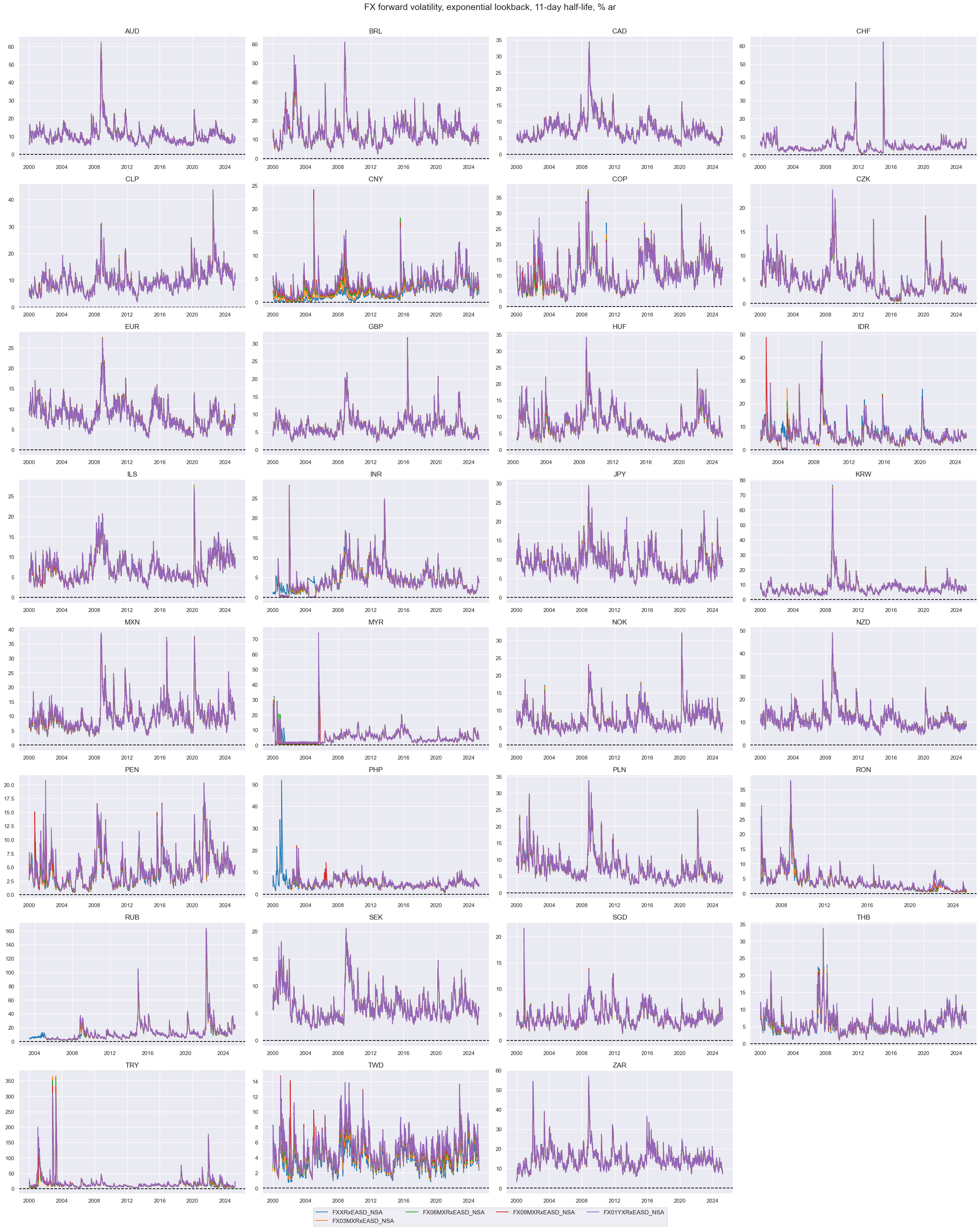
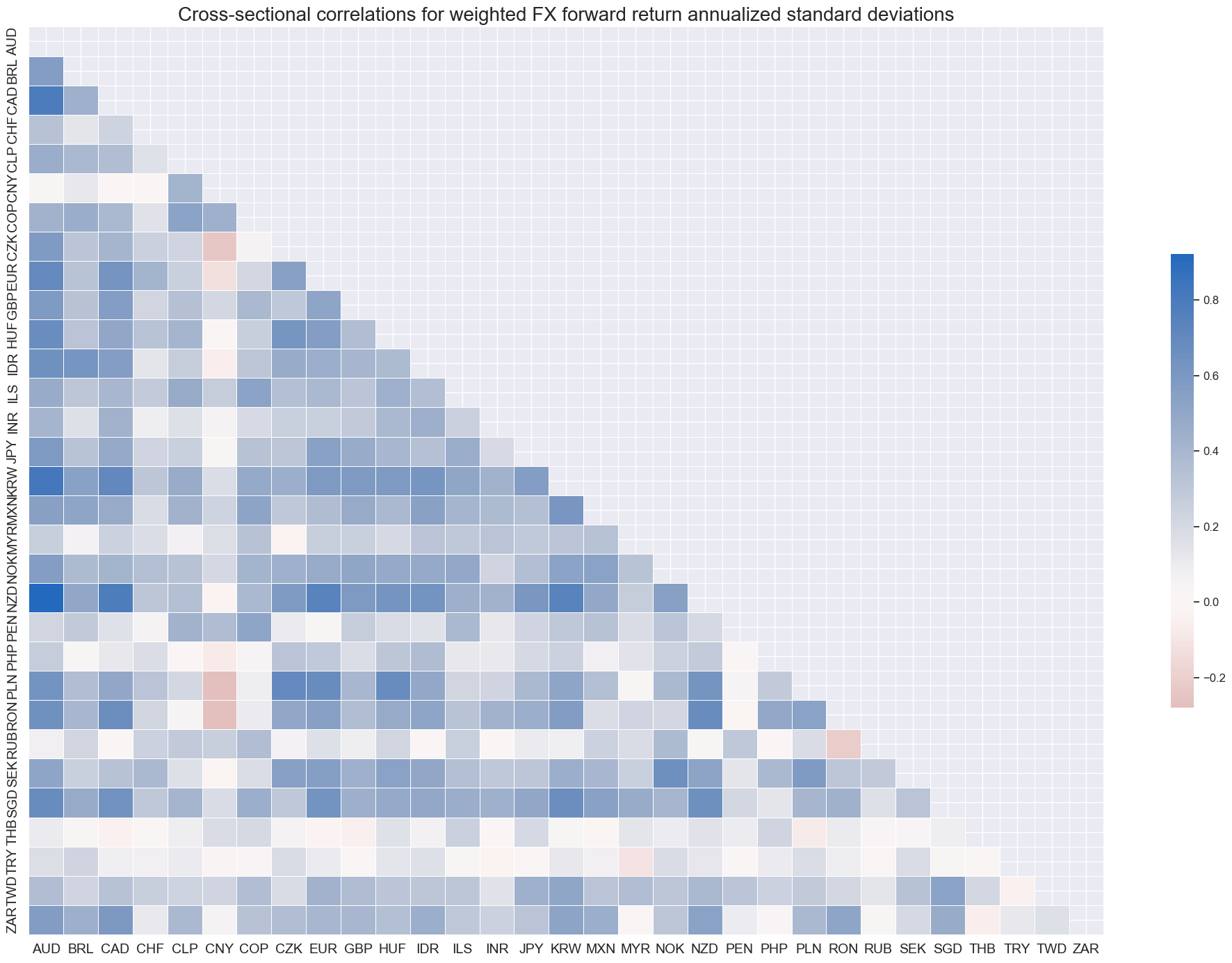
Correlation of FX volatility has been positive across currencies. However, CNY, which has been heavily managed by an effective exchange rate target, has been a notable exception. Also USDTRY/EURTRY and USDTHB forward volatility have been only weakly correlated with other volatilities.
xcatx = "FXXRxEASD_NSA"
cidx = cids_exp

msp.correl_matrix(
    df,
    xcats=xcatx,
    cids=cidx,
    title="Cross-sectional correlations for weighted FX forward return annualized standard deviations",
    size=(20, 14),
)
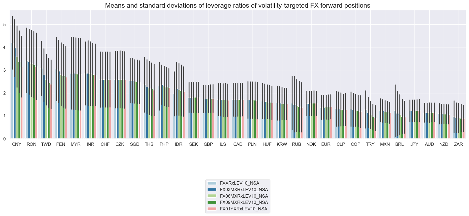
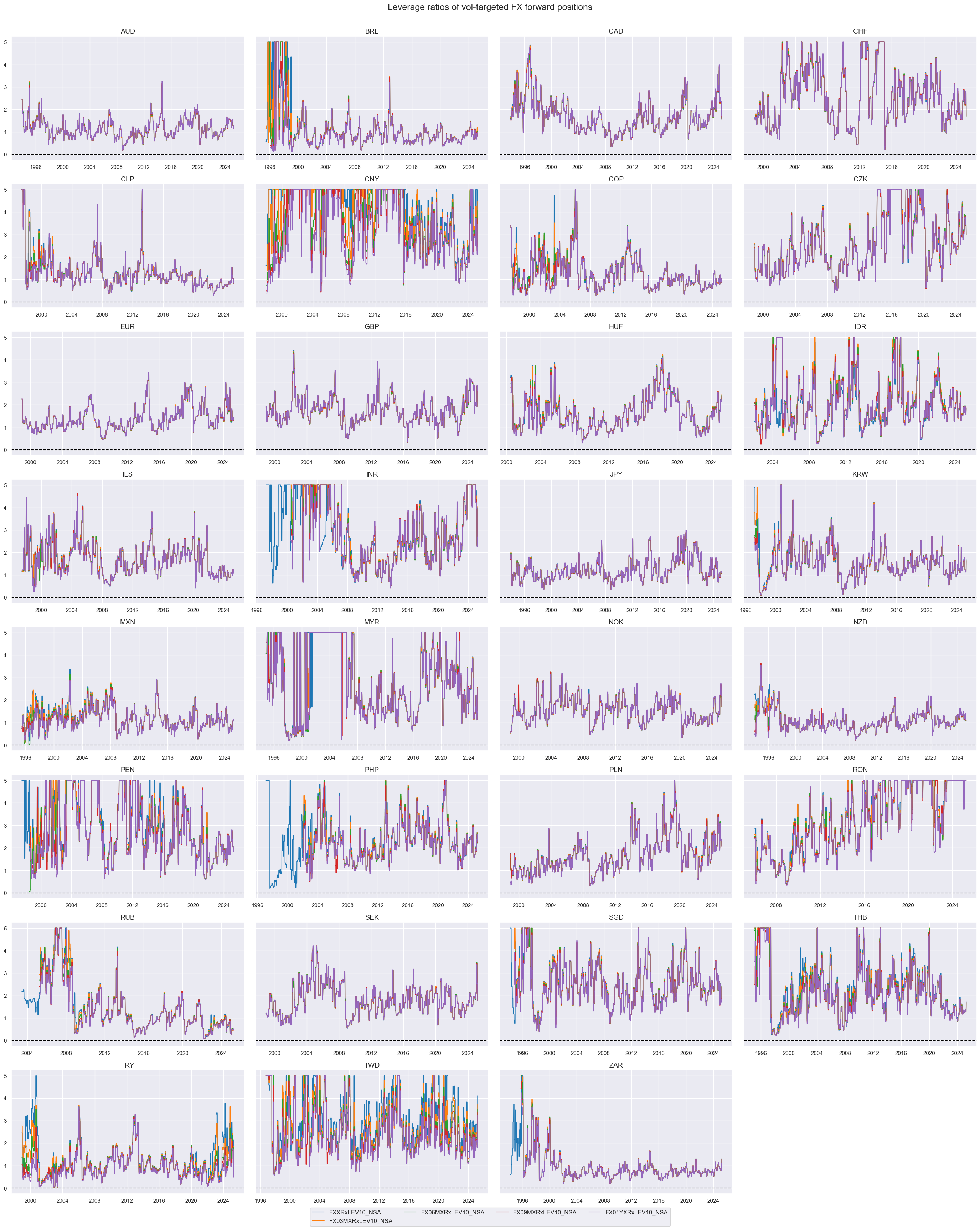
Leverage ratios of vol-targeted FX forward positions #
Average leverage ratios across currencies have ranged from less than 1 to close to 4. The upper boundary of 5x leverage is typically reached in currency areas and periods of tight exchange rate targeting.
xcatx = [
    "FXXRxLEV10_NSA", "FX03MXRxLEV10_NSA", "FX06MXRxLEV10_NSA", "FX09MXRxLEV10_NSA", "FX01YXRxLEV10_NSA",
    ]
cidx = cids_exp

msp.view_ranges(
    df,
    xcats=xcatx,
    cids=cidx,
    sort_cids_by="mean",
    start=start_date,
    kind="bar",
    title="Means and standard deviations of leverage ratios of volatility-targeted FX forward positions",
    size=(16, 8),
)
xcatx = [
    "FXXRxLEV10_NSA", "FX03MXRxLEV10_NSA", "FX06MXRxLEV10_NSA", "FX09MXRxLEV10_NSA", "FX01YXRxLEV10_NSA",
]
cidx = cids_exp

msp.view_timelines(
    df,
    xcats=xcatx,
    cids=cidx,
    start=start_date,
    title="Leverage ratios of vol-targeted FX forward positions",
    ncol=4,
    same_y=True,
    size=(12, 7),
    all_xticks=True,
)
Importance #
Research Links #
on importance of financial market volatility in asset pricing/asset allocation
“It is generally known that financial market volatility is central to the theory and practice of asset pricing, asset allocation, and risk management” Jiang, Han & Yin
“First, uncertainty measures provide a basis for comparing the market’s assessment of risk with private information and research. Second, changes in uncertainty indicators often predict near-term flows in and out of risky asset classes. Third, the level of public and market uncertainty is indicative of risk premia offered across asset classes.” Macrosynergy
“A positive and significant relationship between FX and stocks return volatilities for all the foreign currencies considered (USD, GBP and JPY) has been found.” Karoui
on FX volatility and FX returns
“… the consideration of volatility is not new, as the 1990s broughtabout many studies examining the role of volatility in explaining time-varying risk premia, unfortunately without a satisfactory result. However, the earlieruse of volatility in modeling currency risk premia has applied a time-series perspective on single exchange rates… In contrast, we rely on asset pricing methods well-establishedin the stock market literature where aggregate volatility innovations serve asa systematic risk factor for the cross section of portfolio returns.” Menkoff, Sarno, Schmeling, and Schrimpf
“We study the cross-section of returns on FX options sorting currencies based on implied volatilities (IVs). A long low IV-short high IV strategy produces large average returns after transaction costs. Total volatility matters rather than any component or transformation of volatility. “ Fullwood, James and Marsh
“… exchange rates and currency returns can be predicted by the dollar exchange rate volatility and the financial CP outstanding, which are both proxies for leverage constraint tightness.” Fang and Liu
“This paper provides empirical evidence of the predictive power of the currency implied volatility term structure (IVTS) for the behavior of the exchange rate from both cross-sectional and time series perspectives. Intriguingly, the direction of the prediction is not the same for developed and emerging markets. For developed markets, a high slope means low future returns, while for emerging markets it means high future returns. “ Ornelas & Mauad
“… real exchange rate volatility an important factor behind bilateral portfolio home bias… we find that a reduction of monthly real exchange rate volatility from its sample mean to zero reduces bond home bias by up to 60 percentage points, while it reduces equity home bias by only 20 percentage points.” Fidora, Fratzscher and Thimann
“Our results indicate that the (change in) implied volatility of equity and currency markets is a strong contemporaneous indicator of returns on currency carry investing. This is consistent with the view that during periods of increasing risk aversions, currency carry trades tend to perform poorly… The (change in) implied volatility on equity or currency markets is a weak predictive indicator of returns on currency carry investing. The changes of implied volatility seem to be better timing indicators than levels of implied volatility.” Egbers & Swinkels
“Variance risk premiums mark the difference between implied (future) and past volatility. They indicate changes in risk aversion or uncertainty. As these changes may differ or have different implications across countries, they may cause FX overshooting and payback. The effect complements the simpler argument that rising currency volatility predicts lower FX carry returns. Academic papers support both effects empirically.” Macrosynergy
Empirical Clues #
dfb = df[df["xcat"].isin(["FXTARGETED_NSA", "FXUNTRADABLE_NSA"])].loc[
    :, ["cid", "xcat", "real_date", "value"]
]
dfba = (
    dfb.groupby(["cid", "real_date"])
    .aggregate(value=pd.NamedAgg(column="value", aggfunc="max"))
    .reset_index()
)
dfba["xcat"] = "FXBLACK"
fxblack = msp.make_blacklist(dfba, "FXBLACK")

dfx= df.copy()
The make_zn_scores() function normalizes positive values, like volatility, around a neutral reference point (e.g., the mean). A zn-score measures how far a value is from this point, scaled by a chosen spread (e.g., standard deviation).
xcatx = ["FXXRxEASD_NSA", "DU10YXRxEASD_NSA", "EQXRxEASD_NSA", "CDS05YXRxEASD_NSA"]

for xcat in xcatx:
    dfa = msp.make_zn_scores(
        dfx,
        xcat=xcat,
        cids=cids,
        neutral="mean",
        sequential=True,
        min_obs=261 * 3,
        pan_weight=1,
        thresh=3,
        postfix="PZ",
        est_freq="m",

    )
    dfx = msm.update_df(dfx, dfa)
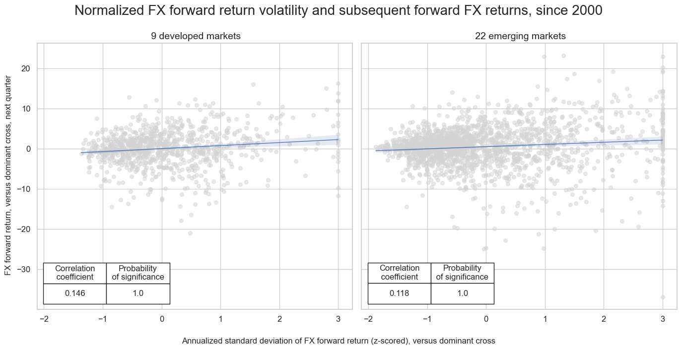
FX volatility and subsequent FX forward returns #
Volatility carries premia in the FX space. In both developed and emerging FX markets there has been a positive relation between realized volatility and subsequent FX forward returns, at a monthly or quarterly frequency. This is consistent with the observation that most investment managers measure asset values in U.S. dollars or euros and that FX volatility increases mark-to-market risk.
sigx = {
     "FXXRxEASD_NSAPZ": "FX forward volatility, z-scored",
 }

targx = {
    "FXXR_NSA": "FX forward return",
}

# Get common cross-section identifiers
cidx = msm.common_cids(dfx, xcats=list(sigx.keys()) + list(targx.keys()))

# Define cross-section (market) groups
cidx_dict = {
    "developed markets": list(set(cids_dmca)),
    "emerging markets": list(set(cids_em)),
}

# Dictionary to store CategoryRelations objects
cr = {}
cids_lengths = {}

# Iterate through markets and matched signals/targets
for cid_name, cid_list in cidx_dict.items():
    # Get common cross-sections specific to this market group
    cidx_filtered = set(cidx) & set(cid_list)

    # Store the number of common cross-sections
    cids_lengths[cid_name] = len(cidx_filtered)

    # Construct dictionary key for storing results
    cr[f"cr_{cid_name}"] = msp.CategoryRelations(
        dfx,
        xcats=list(sigx.keys()) + list(targx.keys()),  # Assign correct signals & targets
        cids=list(cidx_filtered),  # Use the corresponding cross-sections for this market
        freq="Q",  # Quarterly frequency
        lag=1,
        xcat_aggs=["last", "sum"],
        blacklist=fxblack,  # Handle optional blacklist
        start="2000-01-01",
    )

# Store all CategoryRelations instances in a list
all_cr_instances = list(cr.values())

subplot_titles = [
    f" {cids_lengths[cid_name]} {cid_name}"
    for cid_name in cidx_dict.keys()  # Iterate over market groups

]
# plot side by side all the CategoryRelations instances
msv.multiple_reg_scatter(
        all_cr_instances,
        title=f"Normalized FX forward return volatility and subsequent forward FX returns, since 2000" ,
        xlab="Annualized standard deviation of FX forward return (z-scored), versus dominant cross",
        ylab="FX forward return, versus dominant cross, next quarter",
        ncol=2,
        nrow=1,
        figsize=(14, 7),
        prob_est="map",
        subplot_titles = subplot_titles,
        coef_box="lower left",
)
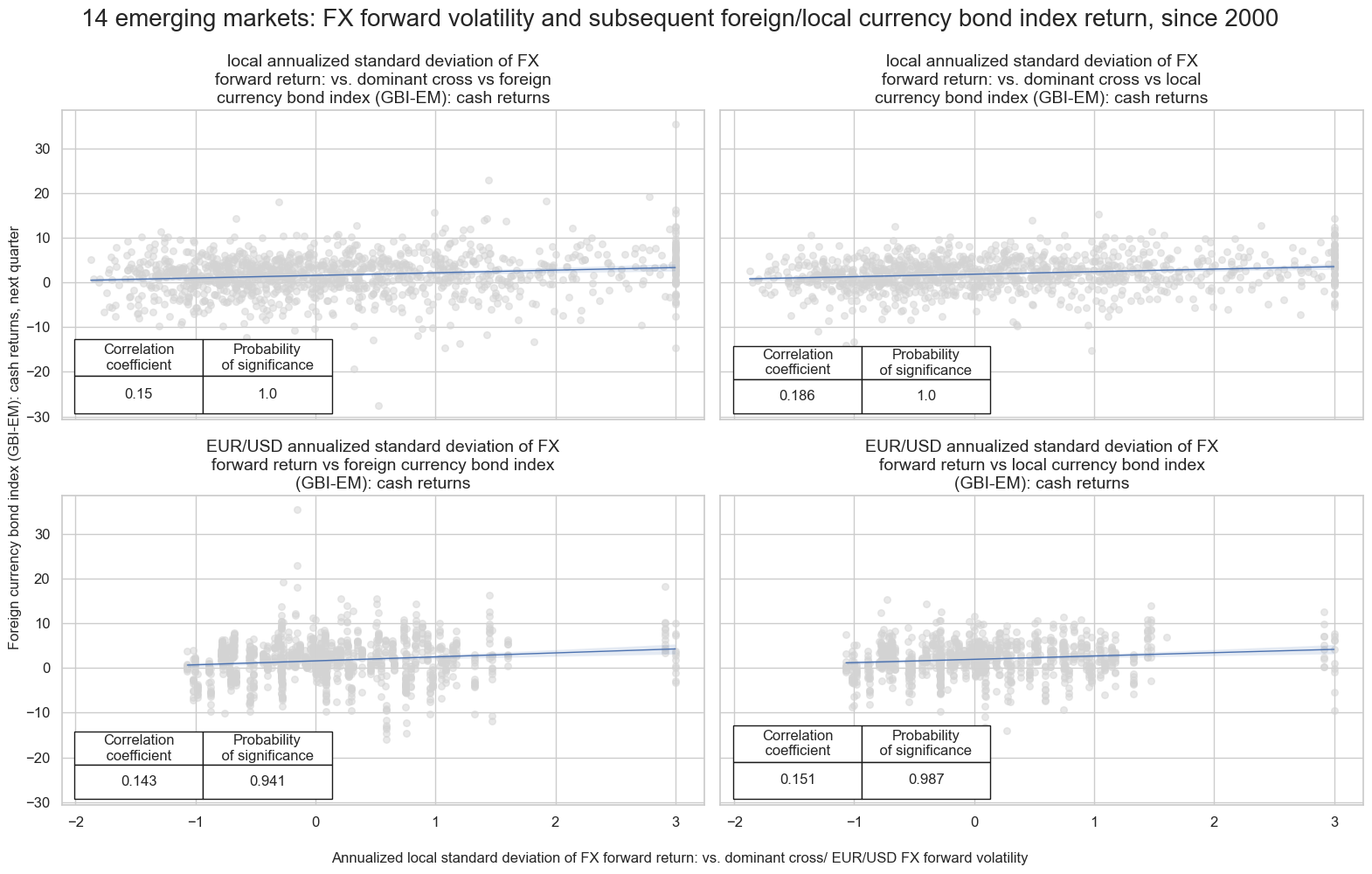
FX volatility and subsequent emerging markets bond index returns #
Both local and EURUSD FX volatility has positively predicted subsequent emerging markets bond index returns, for both local-currency and foreign-currency indices. The predictive power has been more significant with respect to local-currency markets. High FX volatility typically translates into elevated risk premia on local bond exposure.
calcs = [
    "iEURFXXRxEASD_NSAPZ = ( iEUR_FXXRxEASD_NSAPZ ) "
  ]

dfa = msp.panel_calculator(dfx, calcs, cids=cids)
dfx = msm.update_df(dfx, dfa)
# Define signal and target mappings
sigx = {
    "FXXRxEASD_NSAPZ": "local annualized standard deviation of FX forward return: vs. dominant cross",
    "iEURFXXRxEASD_NSAPZ": "EUR/USD annualized standard deviation of FX forward return",

  }

targx = {
    "FCBIR_NSA": "foreign currency bond index (GBI-EM): cash returns",
    "LCBIR_NSA": "local currency bond index (GBI-EM): cash returns",
  }

# Define cross-section (market) groups
cidx = msm.common_cids(dfx, xcats=list(sigx.keys()) + list(targx.keys()))
cidx_dict = {
    "emerging markets": list(set(cids_em) & set(cidx)),
     }

# Dictionary to store CategoryRelations objects
cr = {}

# Iterate through markets and matched signals/targets
for sig_name in sigx.keys():  # Use the actual category names
    for targ_name in targx.keys():
      for cid_name, cid_list in cidx_dict.items():
        cr[f"cr_{sig_name}_{targ_name}_{cid_name}"] = msp.CategoryRelations(
                dfx,
                xcats=[sig_name, targ_name],
                cids=cid_list,
                freq="Q",
                lag=1,
                xcat_aggs=["last", "sum"],
                blacklist=fxblack,
                start="2000-01-01",
               # xcat_trims=[40, 5],
            )

# Store all CategoryRelations instances in a list
all_cr_instances = list(cr.values())

subplot_titles = [
    f"{sigx[sig_key]} vs {targx[targ_key]}"
    for sig_key in sigx.keys()
    for targ_key in targx.keys()
]

# plot side by side all the CategoryRelations instances
msv.multiple_reg_scatter(
        all_cr_instances,
        title=f"{len(list(set(cids_em) & set(cidx)))} emerging markets: FX forward volatility and subsequent foreign/local currency bond index return, since 2000" ,
        xlab="Annualized local standard deviation of FX forward return: vs. dominant cross/ EUR/USD FX forward volatility",
        ylab="Foreign currency bond index (GBI-EM): cash returns, next quarter",
        ncol=2,
        nrow=2,
        figsize=(16, 10),
        prob_est="map",
        subplot_titles = subplot_titles,
        coef_box="lower left",
)
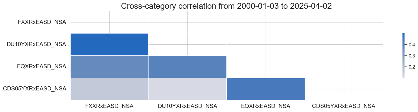
Correlation of asset class volatilities #
FX forward returns volatility is strongly correlated with other asset classes` volatilities, such as CDS, equity index, and duration volatility. This relationship holds true across both emerging and developed markets. The strongest relations rate between FX and rates volatility and between equity and CDS volatility.
xcatx = ["FXXRxEASD_NSA", "DU10YXRxEASD_NSA", "EQXRxEASD_NSA", "CDS05YXRxEASD_NSA"]
msp.correl_matrix(
    dfx,
    xcats=xcatx,
    cids=cids_dmca + cids_em,
    freq="M",
    size=(16, 4),
    cluster=True,
)

# Get list of blacklisted currency IDs
fxblack_cids = list(fxblack.keys())

# Apply the blacklist to all xcats
blacklist = {xcat: fxblack_cids for xcat in xcatx}

msp.view_timelines(
    dfx,
    xcats=xcatx,
    cids=cids_dmca + cids_em,
    start="2000-01-01",
    ncol=4,
    same_y=False,
    size=(12, 7),
    all_xticks=True,

)
Appendices #
Appendix 1: Currency symbols #
The word ‘cross-section’ refers to currencies, currency areas or economic areas. In alphabetical order, these are AUD (Australian dollar), BRL (Brazilian real), CAD (Canadian dollar), CHF (Swiss franc), CLP (Chilean peso), CNY (Chinese yuan renminbi), COP (Colombian peso), CZK (Czech Republic koruna), DEM (German mark), ESP (Spanish peseta), EUR (Euro), FRF (French franc), GBP (British pound), HKD (Hong Kong dollar), HUF (Hungarian forint), IDR (Indonesian rupiah), ITL (Italian lira), JPY (Japanese yen), KRW (Korean won), MXN (Mexican peso), MYR (Malaysian ringgit), NLG (Dutch guilder), NOK (Norwegian krone), NZD (New Zealand dollar), PEN (Peruvian sol), PHP (Phillipine peso), PLN (Polish zloty), RON (Romanian leu), RUB (Russian ruble), SEK (Swedish krona), SGD (Singaporean dollar), THB (Thai baht), TRY (Turkish lira), TWD (Taiwanese dollar), USD (U.S. dollar), ZAR (South African rand).