Equity index future volatility #
This category group includes measures of realized return volatility for major developed and emerging countries’ local-currency equity index futures. It also includes related generic leverage ratios for volatility targets.
Equity index future volatility #
Ticker : EQXRxEASD_NSA
Label : Estimated annualized standard deviation of equity index future return.
Definition : Annualized standard deviation of equity index future return, % of notional, based on exponential moving average of daily returns.
Notes :
-
The standard deviation is calculated based on an exponential moving average of daily returns with a half-life of 11 active trading days.
-
The return is the % change in the futures price. The return calculation assumes rolling futures (from front to second) on IMM (international monetary markets) days.
-
See Appendix 1 for the list of equity indicies used for each currency area in futures return calculations.
Alternative equity index future volatility #
Ticker : EQNASDAQXRxEASD_NSA / EQRUSSELLXRxEASD_NSA / EQTOPIXXRxEASD_NSA / EQHANGSENGXRxEASD_NSA
Label : Estimated annualized standard deviation of equity index future return: NASDAQ 100 / Russell 2000 / TOPIX / Hang Seng.
Definition : Annualized standard deviation of equity index future return, % of notional, based on exponential moving average of daily returns: NASDAQ 100 / Russell 2000 / TOPIX / Hang Seng.
Notes :
-
Alternative indices are not the main equity index of the country but are available for suplementary analyses.
-
See Appendix 2 for the list of alternative equity indices used. Alternative indices are available for HKD, JPY, and USD.
-
See the important notes under “Equity index future volatility” (
EQXRxEASD_NSA).
Leverage ratio of vol-targeted equity future position #
Ticker : EQXRxLEV10_NSA
Label : Leverage ratio of equity index future position for 10% annualized vol target.
Definition : Equity index future leverage for a 10% annualized vol target, as a ratio of contract notional relative to risk capital on which the return is calculated.
Notes :
-
This serves as the leverage ratio for a 10% annualized vol target and is inversely proportional to the estimated annualized standard deviation of the return on a USD1 notional position. The leverage can viewed as indicative for positioning and endogenous market risk.
-
See further the notes for “Equity index future volatility” (
EQXRxEASD_NSA).
Leverage ratio of vol-targeted alternative equity future position #
Ticker : EQNASDAQXRxLEV10_NSA / EQRUSSELLXRxLEV10_NSA / EQTOPIXXRxLEV10_NSA / EQHANGSENGXRxLEV10_NSA
Label : Leverage ratio of alternative equity index future position for 10% annualized vol target: NASDAQ 100 / Russell 2000 / TOPIX / Hang Seng.
Definition : Alternative equity index future leverage for a 10% annualized vol target, as a ratio of contract notional relative to risk capital on which the return is calculated: NASDAQ 100 / Russell 2000 / TOPIX / Hang Seng.
Notes :
-
See further the notes for “Equity index future volatility” (
EQXRxLEV10_NSA).
Imports #
Only the standard Python data science packages and the specialized
macrosynergy
package are needed.
import os
import numpy as np
import pandas as pd
import matplotlib.pyplot as plt
import seaborn as sns
import math

import json
import yaml

import macrosynergy.management as msm
import macrosynergy.panel as msp
import macrosynergy.signal as mss
import macrosynergy.pnl as msn


from macrosynergy.download import JPMaQSDownload

from timeit import default_timer as timer
from datetime import timedelta, date, datetime

import warnings

warnings.simplefilter("ignore")
The
JPMaQS
indicators we consider are downloaded using the J.P. Morgan Dataquery API interface within the
macrosynergy
package. This is done by specifying
ticker strings
, formed by appending an indicator category code
<category>
to a currency area code
<cross_section>
. These constitute the main part of a full quantamental indicator ticker, taking the form
DB(JPMAQS,<cross_section>_<category>,<info>)
, where
<info>
denotes the time series of information for the given cross-section and category. The following types of information are available:
-
valuegiving the latest available values for the indicator -
eop_lagreferring to days elapsed since the end of the observation period -
mop_lagreferring to the number of days elapsed since the mean observation period -
gradedenoting a grade of the observation, giving a metric of real time information quality.
After instantiating the
JPMaQSDownload
class within the
macrosynergy.download
module, one can use the
download(tickers,start_date,metrics)
method to easily download the necessary data, where
tickers
is an array of ticker strings,
start_date
is the first collection date to be considered and
metrics
is an array comprising the times series information to be downloaded.
# Cross-sections of interest

cids_dmeq = ["AUD", "CAD", "CHF", "EUR", "GBP", "JPY", "SEK", "USD"]
cids_eueq = ["DEM", "ESP", "FRF", "ITL", "NLG"]
cids_aseq = ["CNY", "HKD", "INR", "KRW", "MYR", "SGD", "THB", "TWD"]
cids_exeq = ["BRL", "TRY", "ZAR"]
cids_nueq = ["MXN", "PLN"]

cids = cids_dmeq + cids_eueq + cids_aseq + cids_exeq + cids_nueq
main = ["EQXRxEASD_NSA", "EQXRxLEV10_NSA"]
econ = ["RIR_NSA", "CABGDPRATIO_NSA_12MMA"]  # economic context
mark = ["EQCRR_NSA", "EQCRR_VT10", "EQXR_NSA", "EQXR_VT10"]  # market links

xcats = main + econ + mark
# Download series from J.P. Morgan DataQuery by tickers

start_date = "1990-01-01"
tickers = [cid + "_" + xcat for cid in cids for xcat in xcats]
alt_tickers = [
    "USD_EQNASDAQXRxEASD_NSA",
    "USD_EQNASDAQXRxLEV10_NSA",
    "USD_EQRUSSELLXRxEASD_NSA",
    "USD_EQRUSSELLXRxLEV10_NSA",
    "JPY_EQTOPIXXRxEASD_NSA",
    "JPY_EQTOPIXXRxLEV10_NSA",
    "HKD_EQHANGSENGXRxEASD_NSA",
    "HKD_EQHANGSENGXRxLEV10_NSA",
]
tickers = tickers + alt_tickers
print(f"Maximum number of tickers is {len(tickers)}")

# Retrieve credentials

client_id: str = os.getenv("DQ_CLIENT_ID")
client_secret: str = os.getenv("DQ_CLIENT_SECRET")

# Download from DataQuery

with JPMaQSDownload(client_id=client_id, client_secret=client_secret) as downloader:
    start = timer()
    assert downloader.check_connection()
    df = downloader.download(
        tickers=tickers,
        start_date=start_date,
        metrics=["value", "eop_lag", "mop_lag", "grading"],
        suppress_warning=True,
        show_progress=True,
    )
    end = timer()

dfd = df

print("Download time from DQ: " + str(timedelta(seconds=end - start)))
Maximum number of tickers is 216
Downloading data from JPMaQS.
Timestamp UTC:  2025-03-05 15:51:04
Connection successful!
Requesting data: 100%|██████████| 44/44 [00:08<00:00,  4.95it/s]
Downloading data: 100%|██████████| 44/44 [00:39<00:00,  1.12it/s]
Some expressions are missing from the downloaded data. Check logger output for complete list.
48 out of 864 expressions are missing. To download the catalogue of all available expressions and filter the unavailable expressions, set `get_catalogue=True` in the call to `JPMaQSDownload.download()`.
Some dates are missing from the downloaded data.
2 out of 9180 dates are missing.
Download time from DQ: 0:00:52.842460
Availability #
cids_exp = cids  # cids expected in category panels
msm.missing_in_df(dfd, xcats=main, cids=cids_exp)
No missing XCATs across DataFrame.
Missing cids for EQXRxEASD_NSA:   []
Missing cids for EQXRxLEV10_NSA:  []
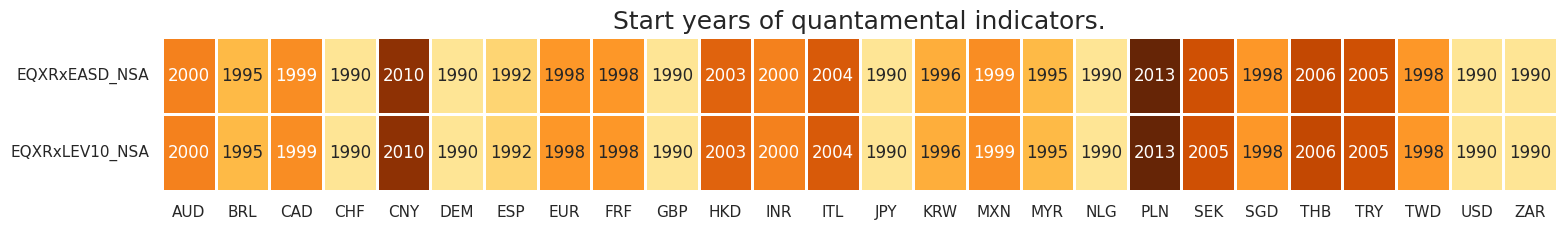
For most currencies, quantamental indicators for equity index future volatility are available by 2000. Notable late-starters are Brazil and Turkey.
For the explanation of currency symbols, which are related to currency areas or countries for which categories are available, please view Appendix 3 .
xcatx = main
cidx = cids_exp

dfx = msm.reduce_df(dfd, xcats=xcatx, cids=cidx)
dfs = msm.check_startyears(
    dfx,
)
msm.visual_paneldates(dfs, size=(18, 2))

print("Last updated:", date.today())
Last updated: 2025-03-05
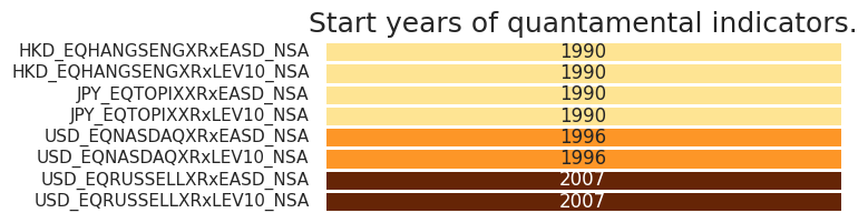
Alternative indicators are available for HKD, JPY and USD. They enable suplementary analyses with different focuses when compared to the country’s main index (small caps, broader/narrower coverage, etc.). All the alternative indices series are available since the 1990s.
alt_cats = [
    "EQNASDAQXRxEASD_NSA",
    "EQNASDAQXRxLEV10_NSA",
    "EQRUSSELLXRxEASD_NSA",
    "EQRUSSELLXRxLEV10_NSA",
    "EQTOPIXXRxEASD_NSA",
    "EQTOPIXXRxLEV10_NSA",
    "EQHANGSENGXRxEASD_NSA",
    "EQHANGSENGXRxLEV10_NSA",
]

dfx = msm.reduce_df(dfd, xcats=alt_cats, cids=cidx)
dfs = msm.check_startyears(
    dfx,
)

# Creating the dataframe for alternative indices
dfs_alt = pd.DataFrame(
    [
        {
            f"{index}_{col}": dfs.loc[index, col]
            for index in dfs.index
            for col in dfs.columns
            if not pd.isna(dfs.loc[index, col])
        }
    ]
)
dfs_alt["idx"] = ""
dfs_alt = dfs_alt.set_index("idx")

msm.visual_paneldates(dfs_alt, size=(6, 2))

print("Last updated:", date.today())
Last updated: 2025-03-05
xcatx = main
cidx = cids_exp
plot = msp.heatmap_grades(
dfd,
xcats=xcatx,
cids=cidx,
size=(18, 2),
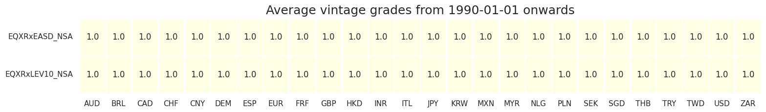
title=f"Average vintage grades from {start_date} onwards",
)
History #
Equity index future volatility #
Historically, volatilities of equity index future returns have not been as diverse across countries as those of currency or interest rate swap positions. The long term averages of countries ranged from less than 15% (annualized) for FTSE Bursa Malaysia KLCI to over 30% for the Hang Seng China Enterprises index.
xcatx = ["EQXRxEASD_NSA"]
cidx = cids_exp

msp.view_ranges(
    dfd,
    xcats=xcatx,
    cids=cidx,
    sort_cids_by="mean",
    start=start_date,
    kind="bar",
    title="Means and standard deviations of equity index future return standard deviations, exponential lookback, % ar, since 2000",
    xcat_labels=["Equity index future volatility"],
    size=(16, 8),
)
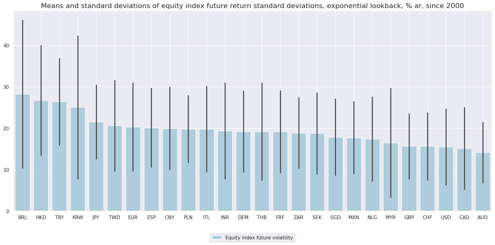
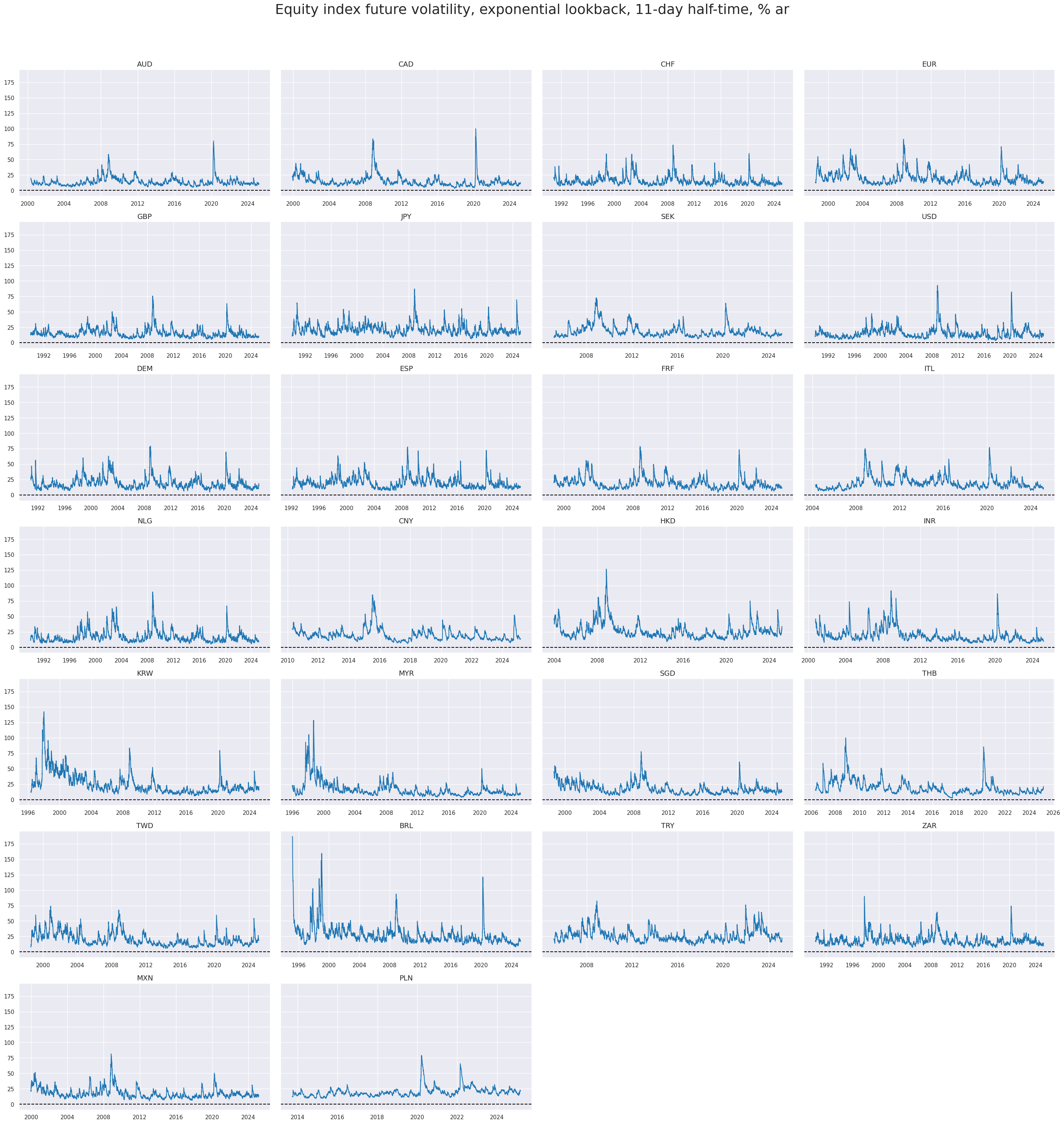
Peak values in crisis episodes post-2000 exceeded 120% (Brazil Bovespa, Nikkei 225 and Hang Seng)!
xcatx = ["EQXRxEASD_NSA"]
cidx = cids_exp

msp.view_timelines(
    dfd,
    xcats=xcatx,
    cids=cidx,
    start=start_date,
    title="Equity index future volatility, exponential lookback, 11-day half-time, % ar",
    title_fontsize=27,
    title_adj=1.02,
    title_xadj=0.5,
    cumsum=False,
    ncol=4,
    same_y=True,
    size=(12, 7),
    aspect=1.7,
    all_xticks=True,
)
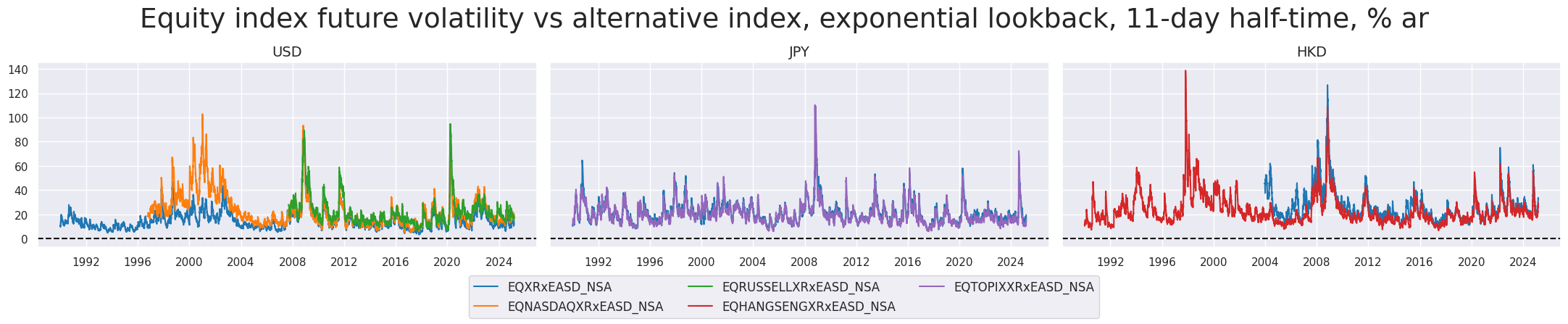
Despite their similarities, alternative indices could reveal distinct risk dynamics throughout history. Unsurprisingly, compared to the S&P 500, the NASDAQ 100 presented much higher volatility during the first years of the 2000s after the dotcom bubble.
msp.view_timelines(
    dfd,
    xcats=["EQXRxEASD_NSA", "EQNASDAQXRxEASD_NSA", "EQRUSSELLXRxEASD_NSA", "EQHANGSENGXRxEASD_NSA", "EQTOPIXXRxEASD_NSA"],
    cids=['USD', 'JPY', 'HKD'],
    start=start_date,
    title="Equity index future volatility vs alternative index, exponential lookback, 11-day half-time, % ar",
    title_fontsize=27,
    title_adj=1.02,
    title_xadj=0.5,
    cumsum=False,
    ncol=4,
    same_y=True,
    size=(12, 7),
    aspect=1.7,
    all_xticks=True,
)
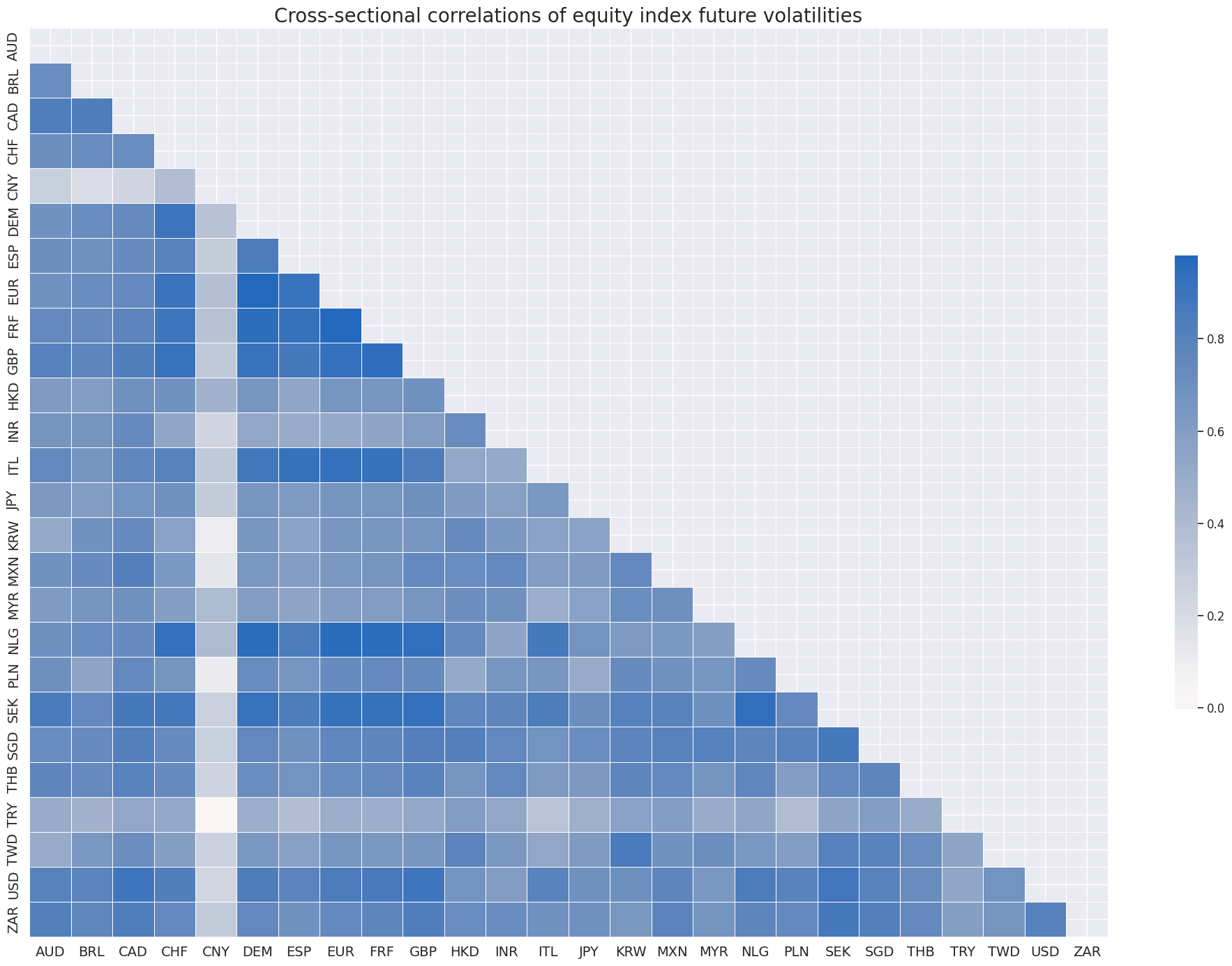
Unsurprisingly, cross-country correlations of equity volatilities have been strongly positive. China’s Shanghai Shenzhen CSI 300 and Poland’s Warsaw General Index 20 have displayed the most idiosyncratic dynamics.
xcatx = "EQXRxEASD_NSA"
cidx = cids_exp

msp.correl_matrix(
    dfd,
    xcats=xcatx,
    cids=cidx,
    title="Cross-sectional correlations of equity index future volatilities",
    size=(20, 14),
)
Leverage ratio of vol-targeted equity future position #
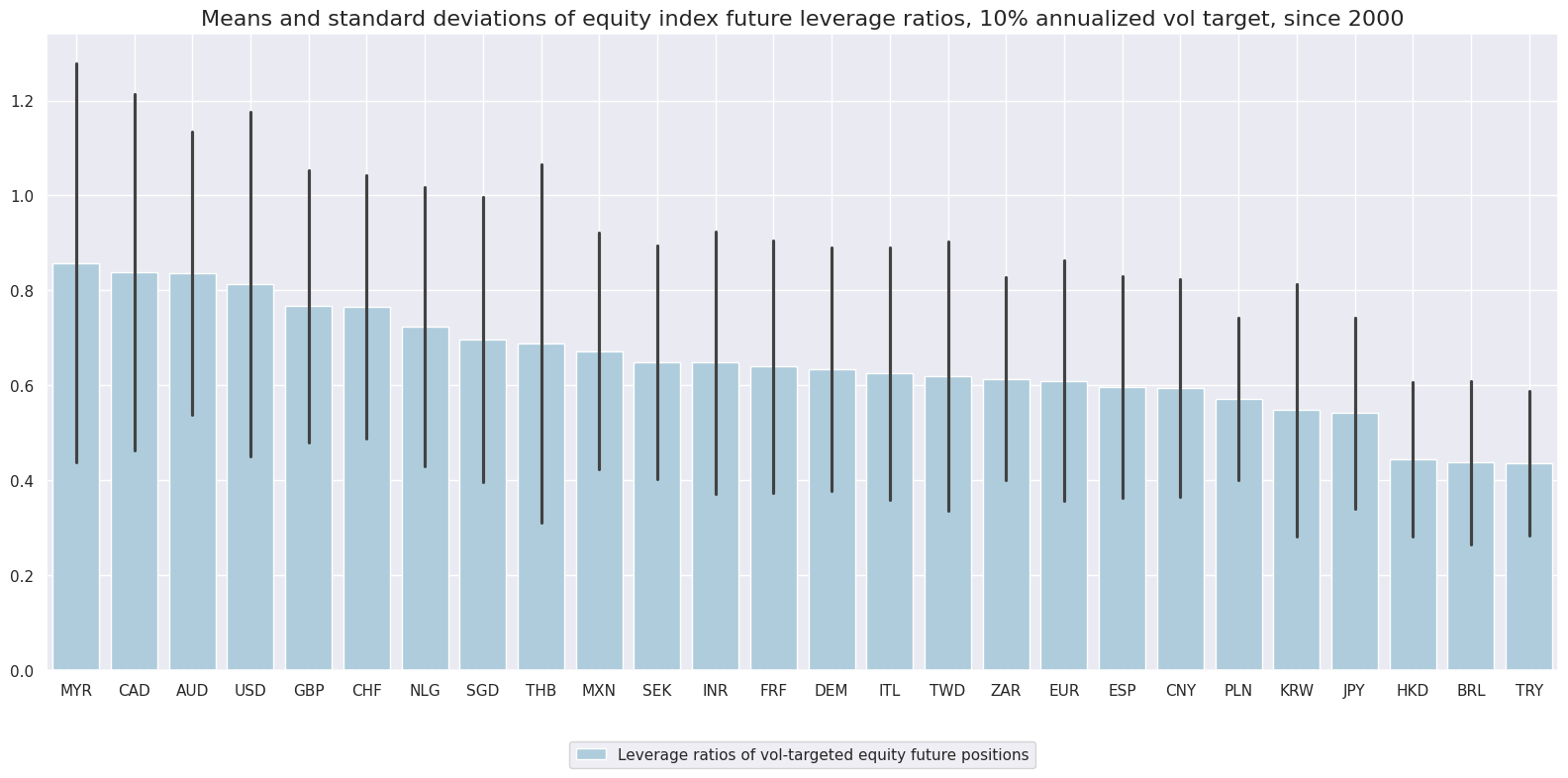
Leverage differences for equal volatility targets across markets have been modest, between 0.4 and 0.9.
xcatx = ["EQXRxLEV10_NSA"]
cidx = cids_exp

msp.view_ranges(
    dfd,
    xcats=xcatx,
    cids=cidx,
    sort_cids_by="mean",
    start=start_date,
    kind="bar",
    title="Means and standard deviations of equity index future leverage ratios, 10% annualized vol target, since 2000",
    xcat_labels=["Leverage ratios of vol-targeted equity future positions"],
    size=(16, 8),
)
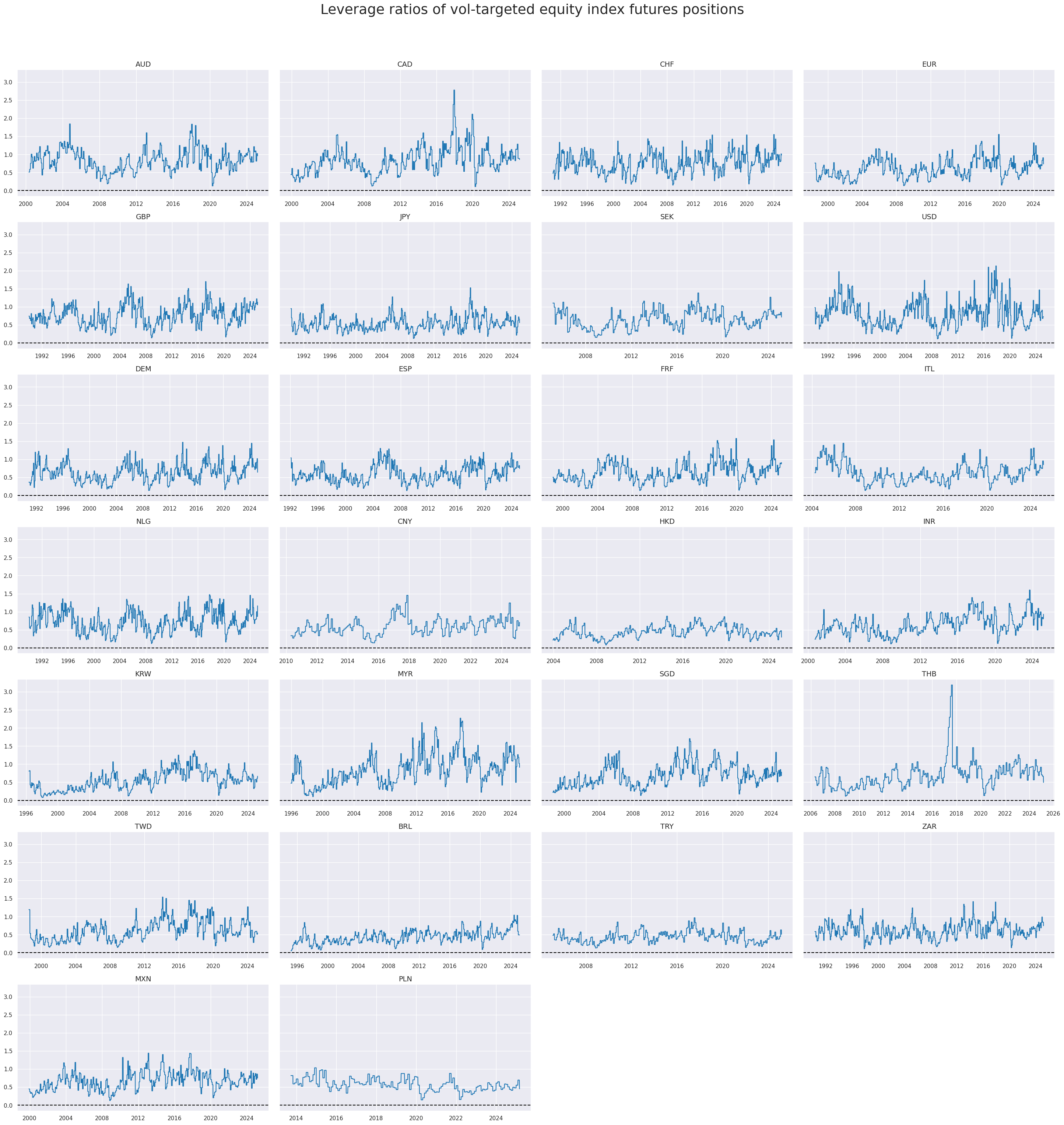
Fluctuations across time have been more sizeable, with leverages ratios in many countries ranging from 0.2 to over 2.
xcatx = ["EQXRxLEV10_NSA"]
cidx = cids_exp

msp.view_timelines(
    dfd,
    xcats=xcatx,
    cids=cidx,
    start=start_date,
    title="Leverage ratios of vol-targeted equity index futures positions",
    title_adj=1.02,
    title_fontsize=27,
    title_xadj=0.5,
    cumsum=False,
    ncol=4,
    same_y=True,
    size=(12, 7),
    aspect=1.7,
    all_xticks=True,
)
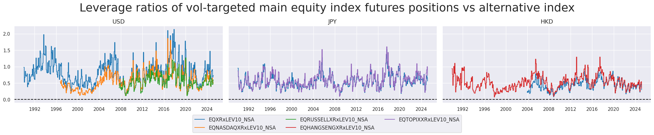
msp.view_timelines(
    dfd,
    xcats=["EQXRxLEV10_NSA", "EQNASDAQXRxLEV10_NSA", "EQRUSSELLXRxLEV10_NSA", "EQHANGSENGXRxLEV10_NSA", "EQTOPIXXRxLEV10_NSA"],
    cids=['USD', 'JPY', 'HKD'],
    start=start_date,
    title="Leverage ratios of vol-targeted main equity index futures positions vs alternative index",
    title_fontsize=27,
    title_adj=1.02,
    title_xadj=0.5,
    cumsum=False,
    ncol=4,
    same_y=True,
    size=(12, 7),
    aspect=1.7,
    all_xticks=True,
)
Importance #
Research Links #
“Equity market volatility can be decomposed into persistent and transitory components by means of statistical methods. The distinction is relevant for macro trading because plausibility and empirical research suggest that the persistent component is associated with macroeconomic fundamentals. This means that persistent volatility is an important signal itself and that its sustainability depends on macroeconomic trends and events. Meanwhile, the transitory component, if correctly identified, is more closely associated with market sentiment and can indicate mean-reverting price dynamics.” Macrosynergy
“Loss aversion implies that risk aversion is changing with market prices. This means that the compensation an investor requires for holding a risky asset varies over time, giving rise to excessive price volatility (relative to the volatility of fundamentals), volatility clustering across time, and predictability of returns. All these phenomena are consistent with historical experience and form a useful basis for trading strategies, such as trend following.” Macrosynergy
“Measures of monetary policy rate uncertainty significantly improve forecasting models for equity volatility and variance risk premia. Theoretically, there is a strong link between the variance of equity returns in present value models and the variance short-term rates. For example, there is natural connection between recent years’ near-zero forward-guided policy rates and low equity volatility. Empirically, the inclusion of derivatives-based measures of short-term rate volatility in regression forecast models for high-frequency realized equity volatility has added significant positive predictive power at weekly, monthly and quarterly horizons.” Macrosynergy
“A long-term empirical study finds two fundamental links between market volatility and financial crises. First, protracted low price volatility leads to a build-up of leverage and risk, making the financial system vulnerable in the medium term (Minsky hypothesis). Second, above-trend volatility indicates (and causes) high uncertainty, impairing investment decisions and raising the near-term crisis risk.” Macrosynergy
Empirical Clues #
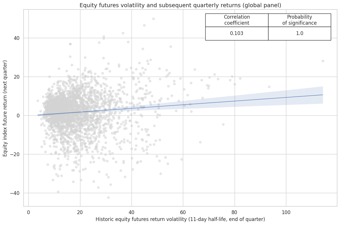
Historically, the correlation between realized equity volatility and subsequent quarterly index future returns has been positive.
xcatx = ["EQXRxEASD_NSA", "EQXR_NSA"]
cidx = cids_exp

cr = msp.CategoryRelations(
    dfd,
    xcats=xcatx,
    cids=cidx,
    freq="Q",
    lag=1,
    xcat_aggs=["last", "sum"],
    start="2000-01-01",
)
cr.reg_scatter(
    title="Equity futures volatility and subsequent quarterly returns (global panel)",
    labels=False,
    coef_box="upper right",
    xlab="Historic equity futures return volatility (11-day half-life, end of quarter)",
    ylab="Equity index future return (next quarter)",
)
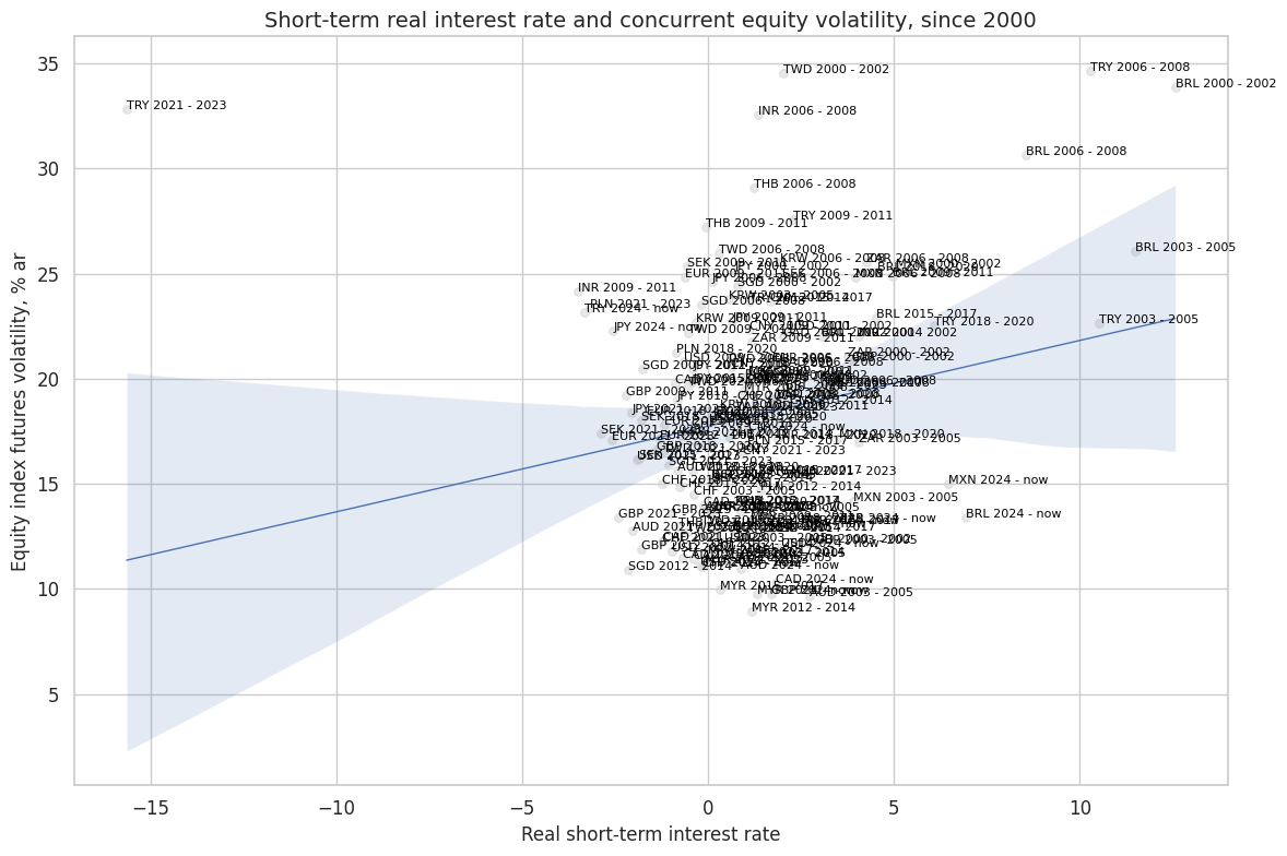
Countries and episodes with higher real interest rates typically coincided with higher equity volatility.
xcatx = ["RIR_NSA", "EQXRxEASD_NSA"]
cidx = cids_exp

cr = msp.CategoryRelations(
    dfd,
    xcats=xcatx,
    cids=cidx,
    freq="M",
    lag=0,
    xcat_aggs=["mean", "mean"],
    start="2000-01-01",
    years=3,
)
cr.reg_scatter(
    title="Short-term real interest rate and concurrent equity volatility, since 2000",
    labels=True,
    xlab="Real short-term interest rate",
    ylab="Equity index futures volatility, % ar",
)
RIR_NSA misses: ['DEM', 'ESP', 'FRF', 'HKD', 'ITL', 'NLG'].
Appendices #
Appendix 1: Equity index specification #
The following equity indices have been used for futures return calculations in each currency area:
-
AUD: Standard and Poor’s / Australian Stock Exchange 200
-
BRL: Brazil Bovespa
-
CAD: Standard and Poor’s / Toronto Stock Exchange 60 Index
-
CHF: Swiss Market (SMI)
-
CNY: Shanghai Shenzhen CSI 300
-
DEM: DAX 30 Performance (Xetra)
-
ESP: IBEX 35
-
EUR: EURO STOXX 50
-
FRF: CAC 40
-
GBP: FTSE 100
-
HKD: Hang Seng China Enterprises
-
INR: CNX Nifty (50)
-
ITL: FTSE MIB Index
-
JPY: Nikkei 225 Stock Average
-
KRW: Korea Stock Exchange KOSPI 200
-
MXN: Mexico IPC (Bolsa)
-
MYR: FTSE Bursa Malaysia KLCI
-
NLG: AEX Index (AEX)
-
PLN: Warsaw General Index 20
-
SEK: OMX Stockholm 30 (OMXS30)
-
SGD: MSCI Singapore (Free)
-
THB: Bangkok S.E.T. 50
-
TRY: Bist National 30
-
TWD: Taiwan Stock Exchange Weighed TAIEX
-
USD: Standard and Poor’s 500 Composite
-
ZAR: FTSE / JSE Top 40
See Appendix 3 for the list of currency symbols used to represent each cross-section.
Appendix 2: Alternative equity index specification #
Alternative equity indices are available for the following currency areas:
-
HKD: Hang Seng
-
JPY: TOPIX
-
USD: NASDAQ 100
-
USD: Russell 2000
See Appendix 3 for the list of currency symbols used to represent each cross-section.
Appendix 3: Currency symbols #
The word ‘cross-section’ refers to currencies, currency areas or economic areas. In alphabetical order, these are AUD (Australian dollar), BRL (Brazilian real), CAD (Canadian dollar), CHF (Swiss franc), CLP (Chilean peso), CNY (Chinese yuan renminbi), COP (Colombian peso), CZK (Czech Republic koruna), DEM (German mark), ESP (Spanish peseta), EUR (Euro), FRF (French franc), GBP (British pound), HKD (Hong Kong dollar), HUF (Hungarian forint), IDR (Indonesian rupiah), ITL (Italian lira), JPY (Japanese yen), KRW (Korean won), MXN (Mexican peso), MYR (Malaysian ringgit), NLG (Dutch guilder), NOK (Norwegian krone), NZD (New Zealand dollar), PEN (Peruvian sol), PHP (Phillipine peso), PLN (Polish zloty), RON (Romanian leu), RUB (Russian ruble), SEK (Swedish krona), SGD (Singaporean dollar), THB (Thai baht), TRY (Turkish lira), TWD (Taiwanese dollar), USD (U.S. dollar), ZAR (South African rand).